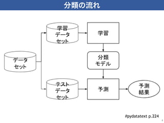
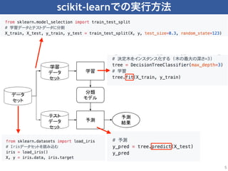
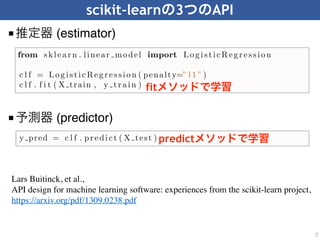
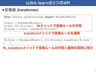
Scikit-learn is a popular machine learning library for Python that provides simple and efficient tools for data mining and data analysis. It includes algorithms for classification, regression, clustering and dimensionality reduction. The scikit-learn API is designed for consistency, with common estimator, predictor and transformer interfaces that allow algorithms to be used interchangeably. This standardized interface helps users easily try different algorithms and preprocessing techniques for their machine learning tasks.

1. scikit-learn
2018 9 25
BPStudy#133
Python

2. ■
■ IT
■
■ /
■
■ twitter: @sfchaos
1

3. Python
■ 2
4.4 scikit-learn
5.2
2

4. scikit-learn
■
3
http://scikit-learn.org/stable/index.html

5. 4
#pydatatext p.224

6. scikit-learn
5

7. or
■
OK
6
■

8. scikit-learn 3 API
■ (estimator)
7
■ (predictor)
able to export a fitted model, using the information from its public attributes,
to an agnostic model description such as PMML (Guazzelli et al., 2009).
To illustrate the initialize-fit sequence, let us consider a supervised learning
task using logistic regression. Given the API defined above, solving this problem
is as simple as the following example.
from sklear n . linear model import Lo g isticReg r essio n
c l f = Lo g isticReg r essio n ( penalty=” l1 ” )
c l f . f i t ( X train , y tr ain )
In this snippet, a LogisticRegression estimator is first initialized by setting the
penalty hyper-parameter to "l1" for ℓ1 regularization. Other hyper-parameters
(such as C, the strength of the regularization) are not explicitly given and thus
set to the default values. Upon calling fit, a model is learned from the training
arrays X train and y train, and stored within the object for later use. Since
all estimators share the same interface, using a different learning algorithm is as
simple as replacing the constructor (the class name); to build a random forest on
the same data, one would simply replace LogisticRegression(penalty="l1")
in the snippet above by RandomForestClassifier().
not require the fit method to perform useful work, implement the estimator
interface. As we will illustrate in the next sections, this design pattern is indeed
of prime importance for consistency, composition and model selection reasons.
2.4 Predictors
The predictor interface extends the notion of an estimator by adding a predict
method that takes an array X test and produces predictions for X test, based on
the learned parameters of the estimator (we call the input to predict “X test”
in order to emphasize that predict generalizes to new data). In the case of
supervised learning estimators, this method typically returns the predicted la-
bels or values computed by the model. Continuing with the previous example,
predicted labels for X test can be obtained using the following snippet:
y pred = c l f . pr edict ( X test )
Some unsupervised learning estimators may also implement the predict in-
terface. The code in the snippet below fits a k-means model with k = 10 on
training data X train, and then uses the predict method to obtain cluster
labels (integer indices) for unseen data X test.
from sklea r n . c l u s t e r import KMeans
km = KMeans( n c l u s t e r s =10)
km. f i t ( X train )
clust pr ed = km. pr edict ( X test )
fit
predict
Lars Buitinck, et al.,
API design for machine learning software: experiences from the scikit-learn project,
https://arxiv.org/pdf/1309.0238.pdf

9. scikit-learn 3 API
■ (transformer)
8
as output a transformed version of X test. Preprocessing, feature selection,
feature extraction and dimensionality reduction algorithms are all provided as
transformers within the library. In our example, to standardize the input X train
to zero mean and unit variance before fitting the logistic regression estimator,
one would write:
from sklear n . pr epr ocessing import StandardScaler
s c a l e r = StandardScaler ()
s c a l e r . f i t ( X train )
X train = s c a l e r . transform ( X train )
Of course, in practice, it is important to apply the same preprocessing to the test
data X test. Since a StandardScaler estimator stores the mean and standard
deviation that it computed for the training set, transforming an unseen test set
X test maps it into the appropriate region of feature space:
X test = s c a l e r . transform ( X test )
Transformers also include a variety of learning algorithms, such as dimension
reduction (PCA, manifold learning), kernel approximation, and other mappings
from one feature space to another.
Additionally, by leveraging the fact that fit always returns the estimator it
was called on, the StandardScaler example above can be rewritten in a single
line using method chaining:
X train = StandardScaler () . f i t ( X train ) . transform ( X train
X train = s c a l e r . transform ( X train )
Of course, in practice, it is important to apply the same preprocessing to the test
data X test. Since a StandardScaler estimator stores the mean and standard
deviation that it computed for the training set, transforming an unseen test set
X test maps it into the appropriate region of feature space:
X test = s c a l e r . transform ( X test )
Transformers also include a variety of learning algorithms, such as dimension
reduction (PCA, manifold learning), kernel approximation, and other mappings
from one feature space to another.
Additionally, by leveraging the fact that fit always returns the estimator it
was called on, the StandardScaler example above can be rewritten in a single
line using method chaining:
X train = StandardScaler () . f i t ( X train ) . transform ( X train
)
Furthermore, every transformer allows fit(X train).transform(X train)
to be written as fit transform(X train). The combined fit transform method
prevents repeated computations. Depending on the transformer, it may skip only
an input validation step, or in fact use a more efficient algorithm for the transfor-
mation. In the same spirit, clustering algorithms provide a fit predict method
that is equivalent to fit followed by predict, returning cluster labels assigned
to the training samples.
fit
transform
fit_transform

10. ■
9
http://scikit-learn.org/stable/modules/generated/
sklearn.svm.SVC.html#sklearn.svm.SVC

11. ■ User Guide
10
http://scikit-learn.org/stable/modules/svm.html#
classification

12. ■User Guide
11
C=1e6 C=0.1
)
•
•
#pydatatext p.231, 232

13. ■
■
■ 3
12

14. ■scikit-learn API
■
1.
2.
■ 2
1
13