Downloaded 177 times


![IMPORTING THE DATASET
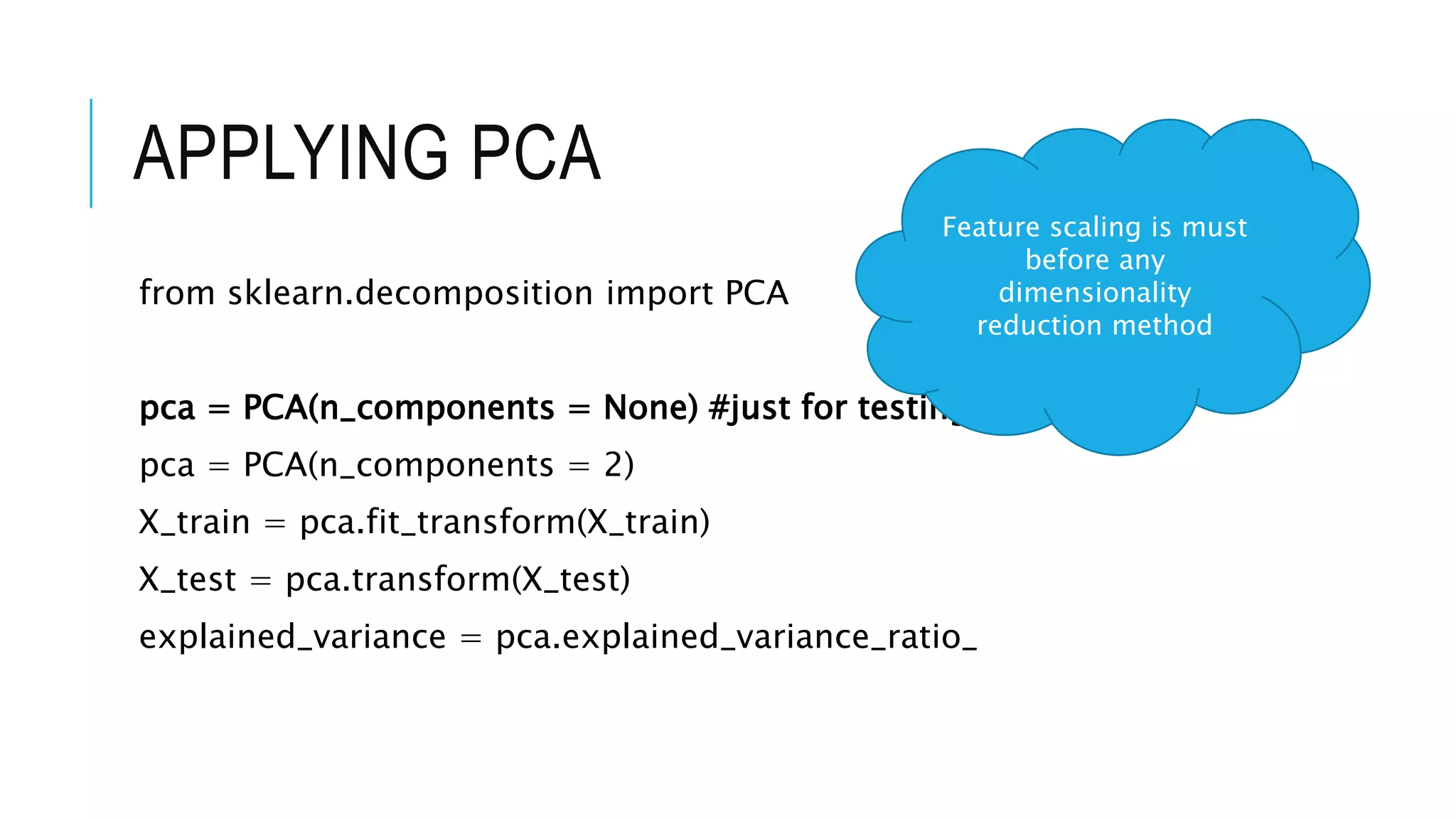
dataset = pd.read_csv('Wine.csv')
X = dataset.iloc[:, 0:13].values
y = dataset.iloc[:, 13].values](https://image.slidesharecdn.com/pcalda-180115144651/75/PCA-and-LDA-in-machine-learning-178-2048.jpg)


![from matplotlib.colors import ListedColormap
X_set, y_set = X_train, y_train
X1, X2 = np.meshgrid(np.arange(start = X_set[:, 0].min() - 1, stop = X_set[:, 0].max() + 1, step = 0.01),
np.arange(start = X_set[:, 1].min() - 1, stop = X_set[:, 1].max() + 1, step = 0.01))
plt.contourf(X1, X2, classifier.predict(np.array([X1.ravel(), X2.ravel()]).T).reshape(X1.shape),
alpha = 0.75, cmap = ListedColormap(('red', 'green', 'blue')))
plt.xlim(X1.min(), X1.max())
plt.ylim(X2.min(), X2.max())
for i, j in enumerate(np.unique(y_set)):
plt.scatter(X_set[y_set == j, 0], X_set[y_set == j, 1],
c = ListedColormap(('red', 'green', 'blue'))(i), label = j)
plt.title('Logistic Regression (Training set)')
plt.xlabel('PC1')
plt.ylabel('PC2')
plt.legend()
plt.show()](https://image.slidesharecdn.com/pcalda-180115144651/75/PCA-and-LDA-in-machine-learning-187-2048.jpg)
![# Visualising the Test set results
from matplotlib.colors import ListedColormap
X_set, y_set = X_test, y_test
X1, X2 = np.meshgrid(np.arange(start = X_set[:, 0].min() - 1, stop = X_set[:, 0].max() + 1, step
= 0.01),
np.arange(start = X_set[:, 1].min() - 1, stop = X_set[:, 1].max() + 1, step = 0.01))
plt.contourf(X1, X2, classifier.predict(np.array([X1.ravel(), X2.ravel()]).T).reshape(X1.shape),
alpha = 0.75, cmap = ListedColormap(('red', 'green', 'blue')))
plt.xlim(X1.min(), X1.max())
plt.ylim(X2.min(), X2.max())
for i, j in enumerate(np.unique(y_set)):
plt.scatter(X_set[y_set == j, 0], X_set[y_set == j, 1],
c = ListedColormap(('red', 'green', 'blue'))(i), label = j)
plt.title('Logistic Regression (Test set)')
plt.xlabel('PC1')
plt.ylabel('PC2')
plt.legend()
plt.show()](https://image.slidesharecdn.com/pcalda-180115144651/75/PCA-and-LDA-in-machine-learning-188-2048.jpg)

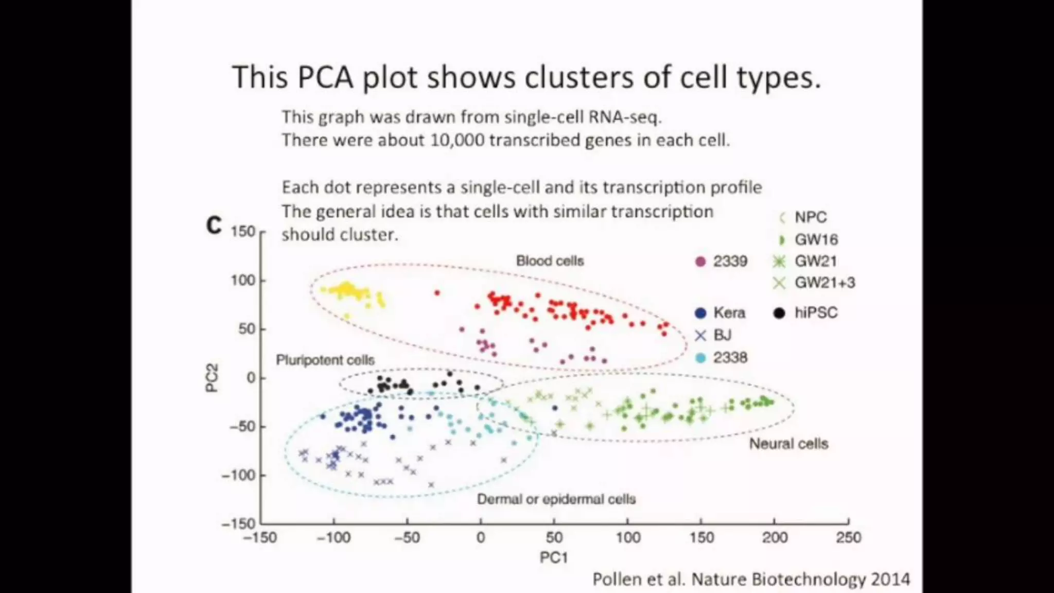
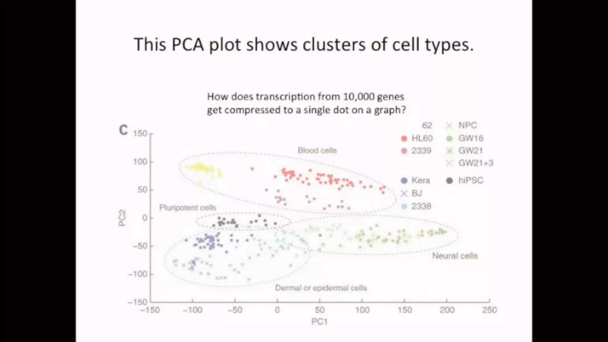
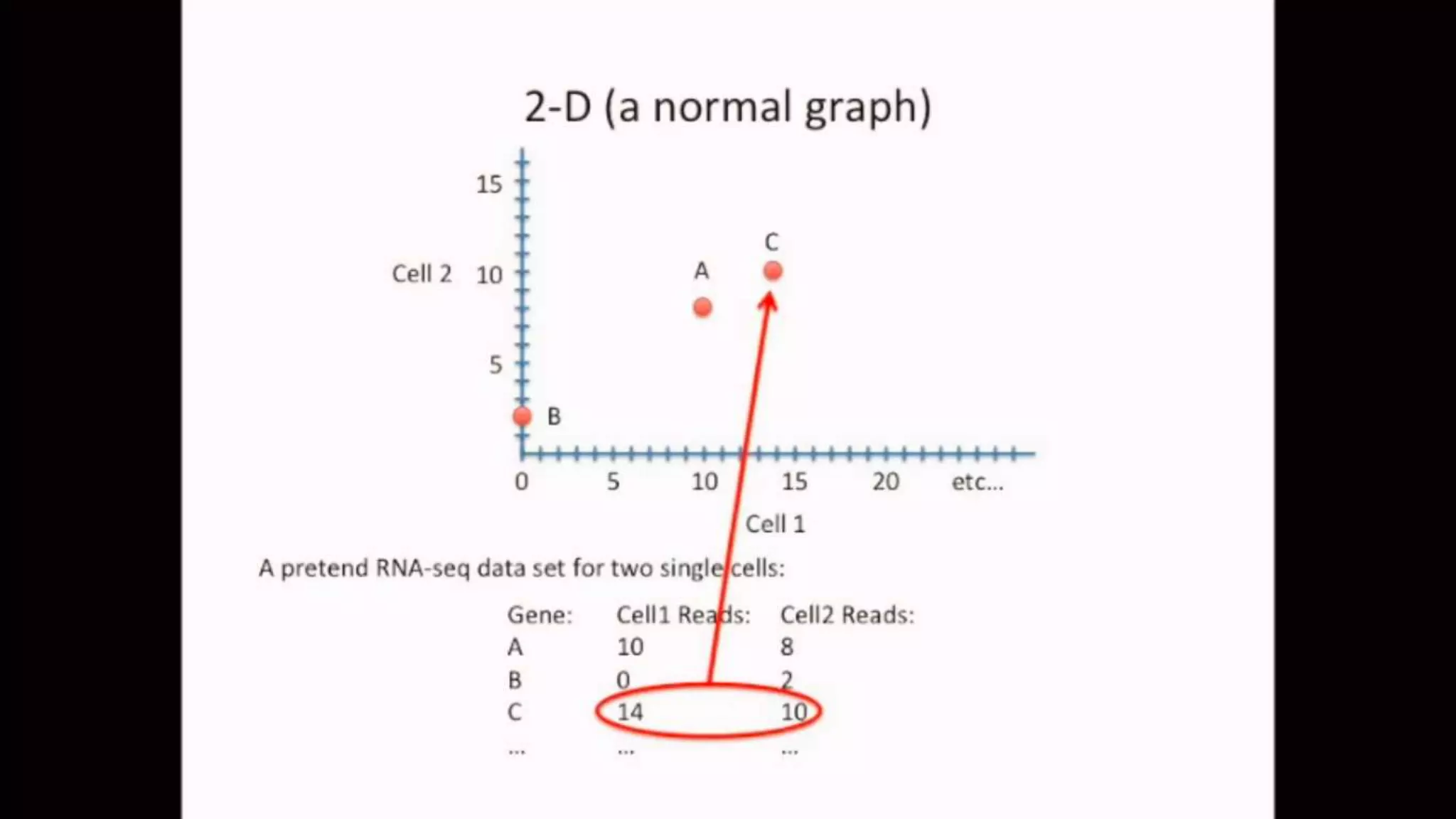
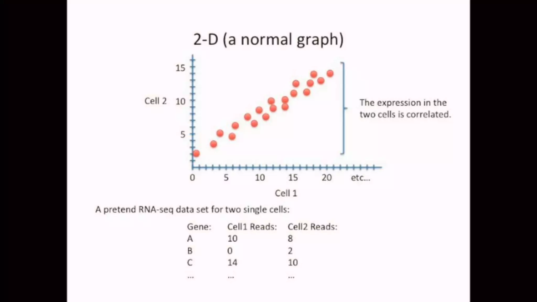
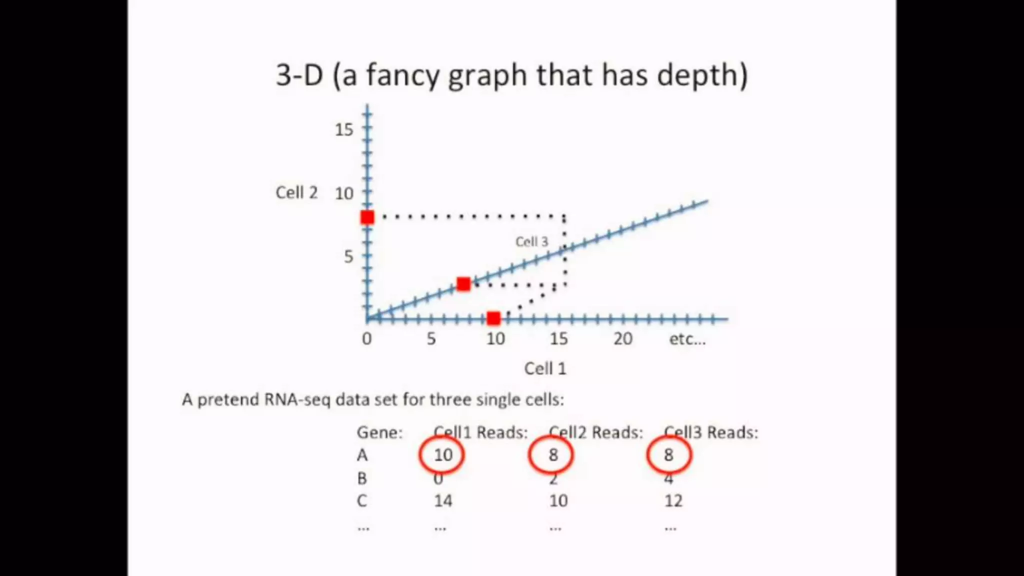
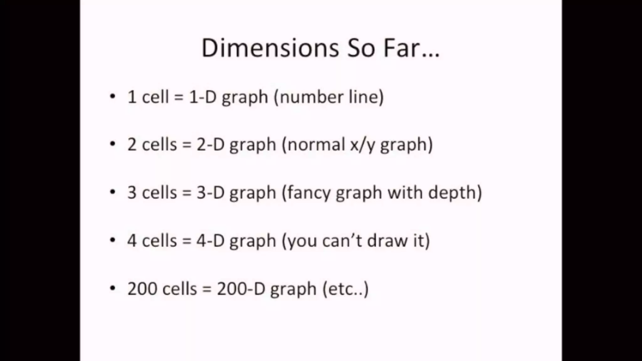
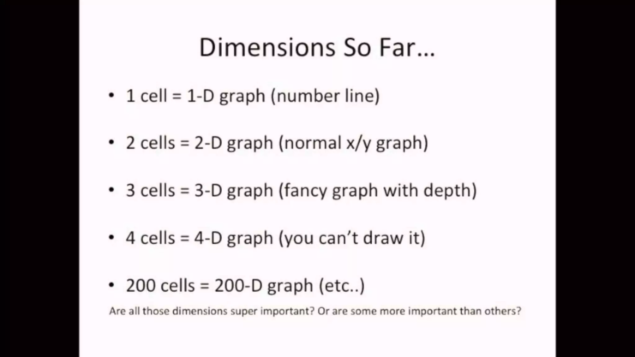
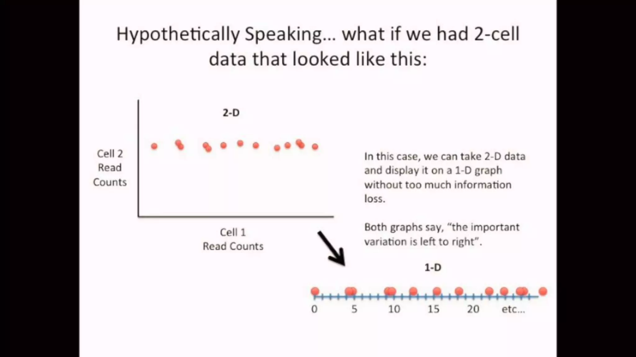
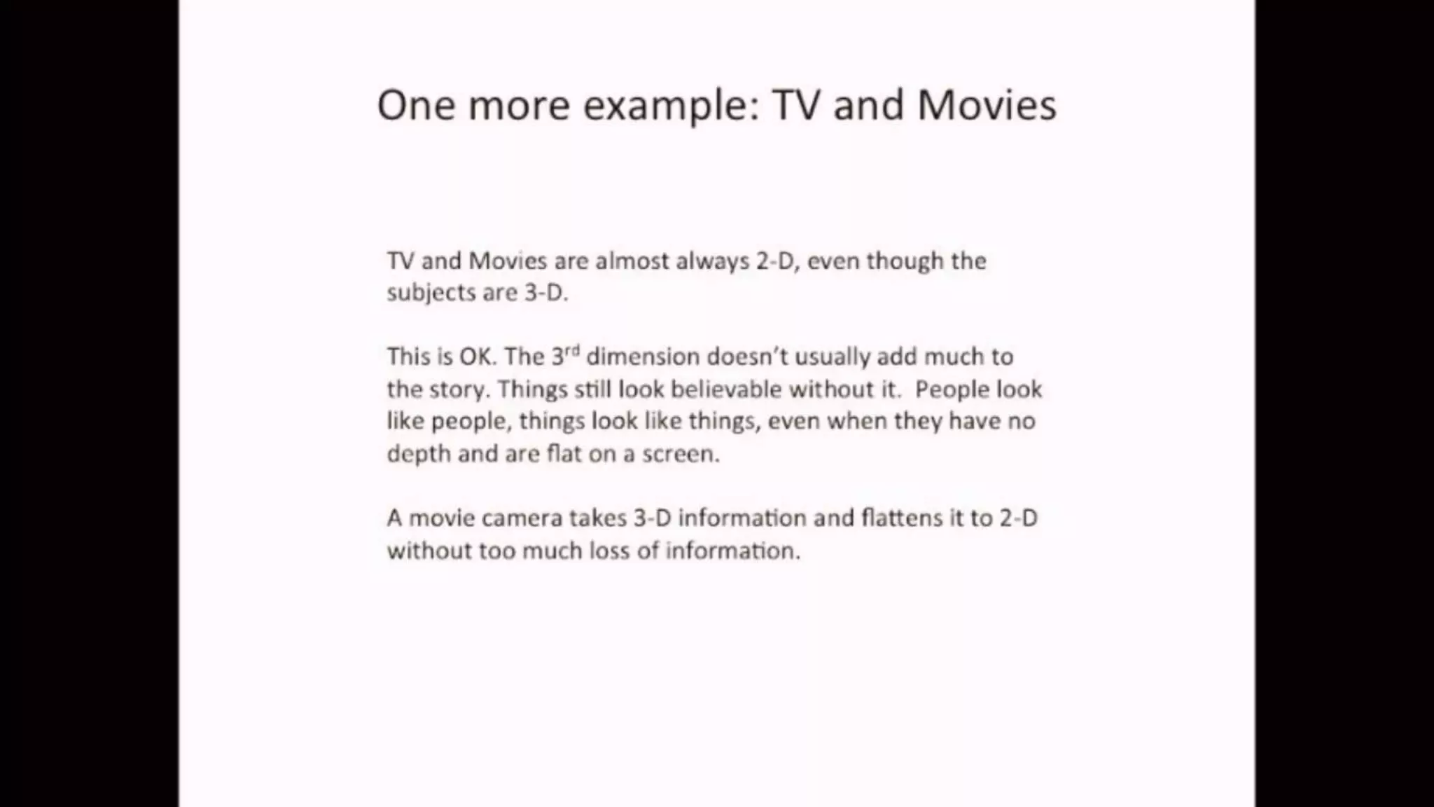
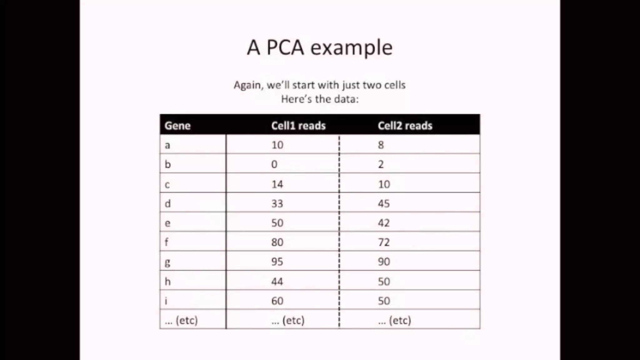
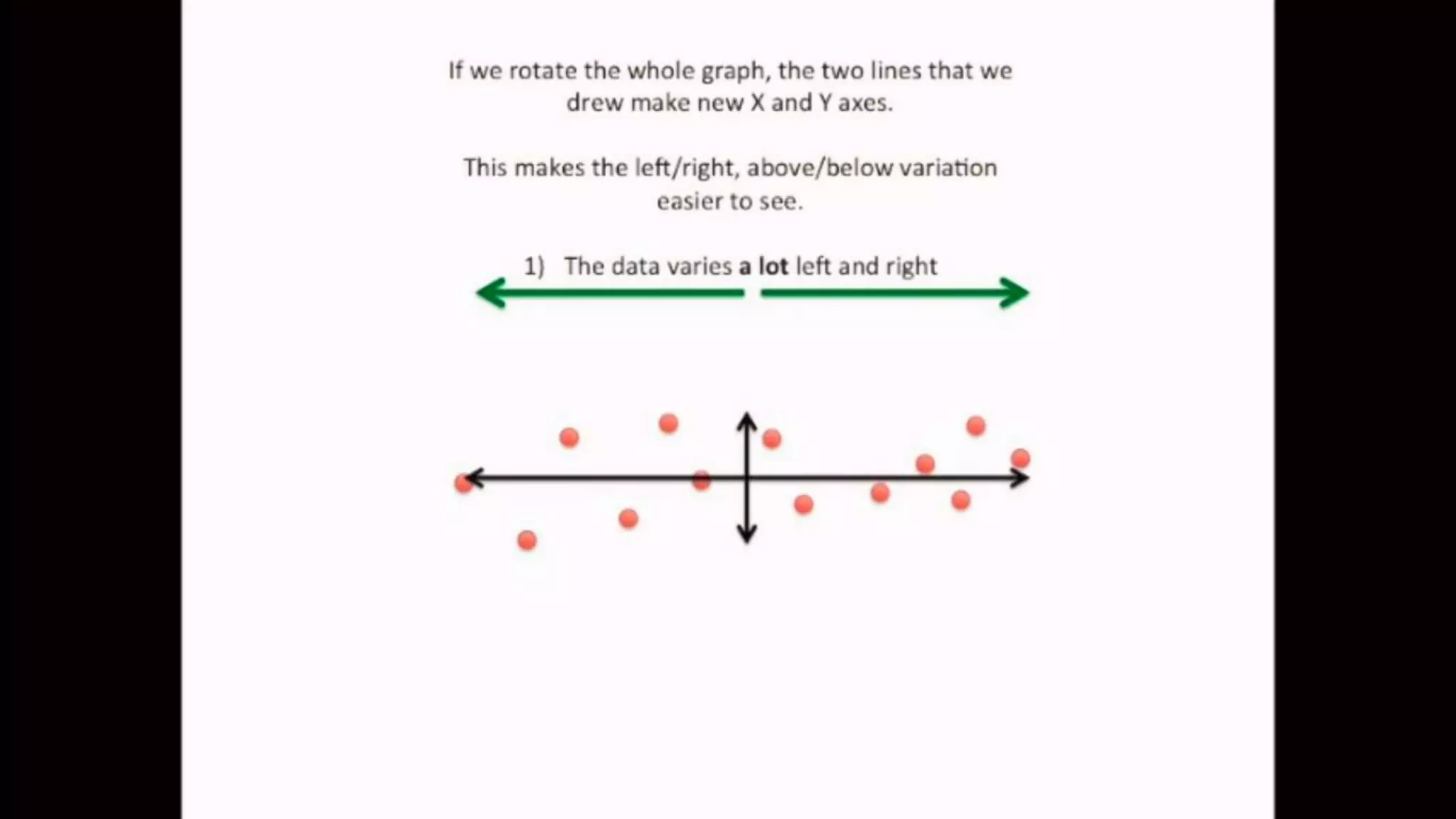
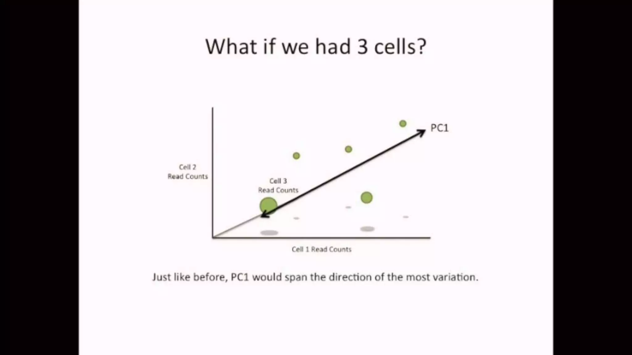
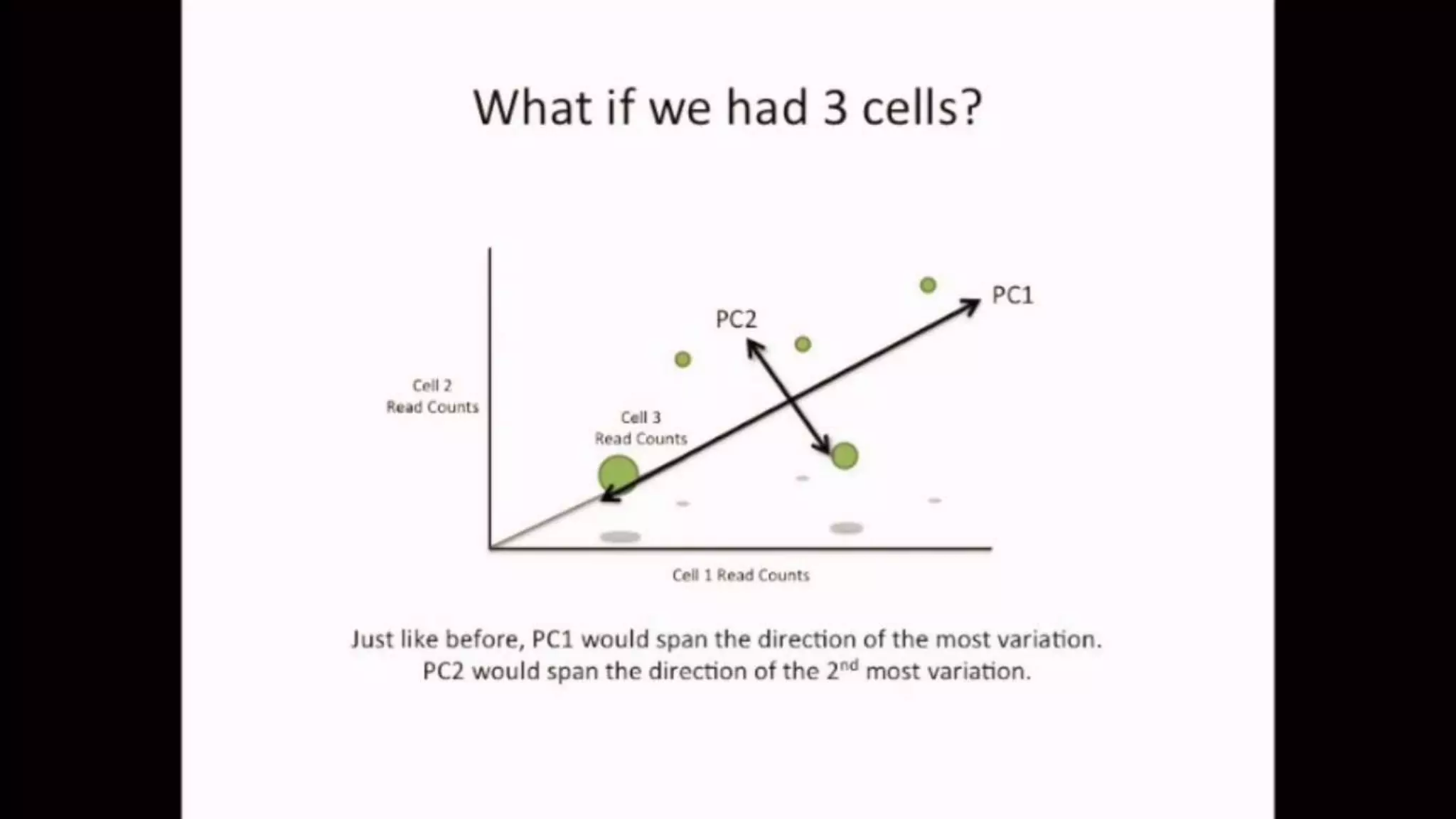
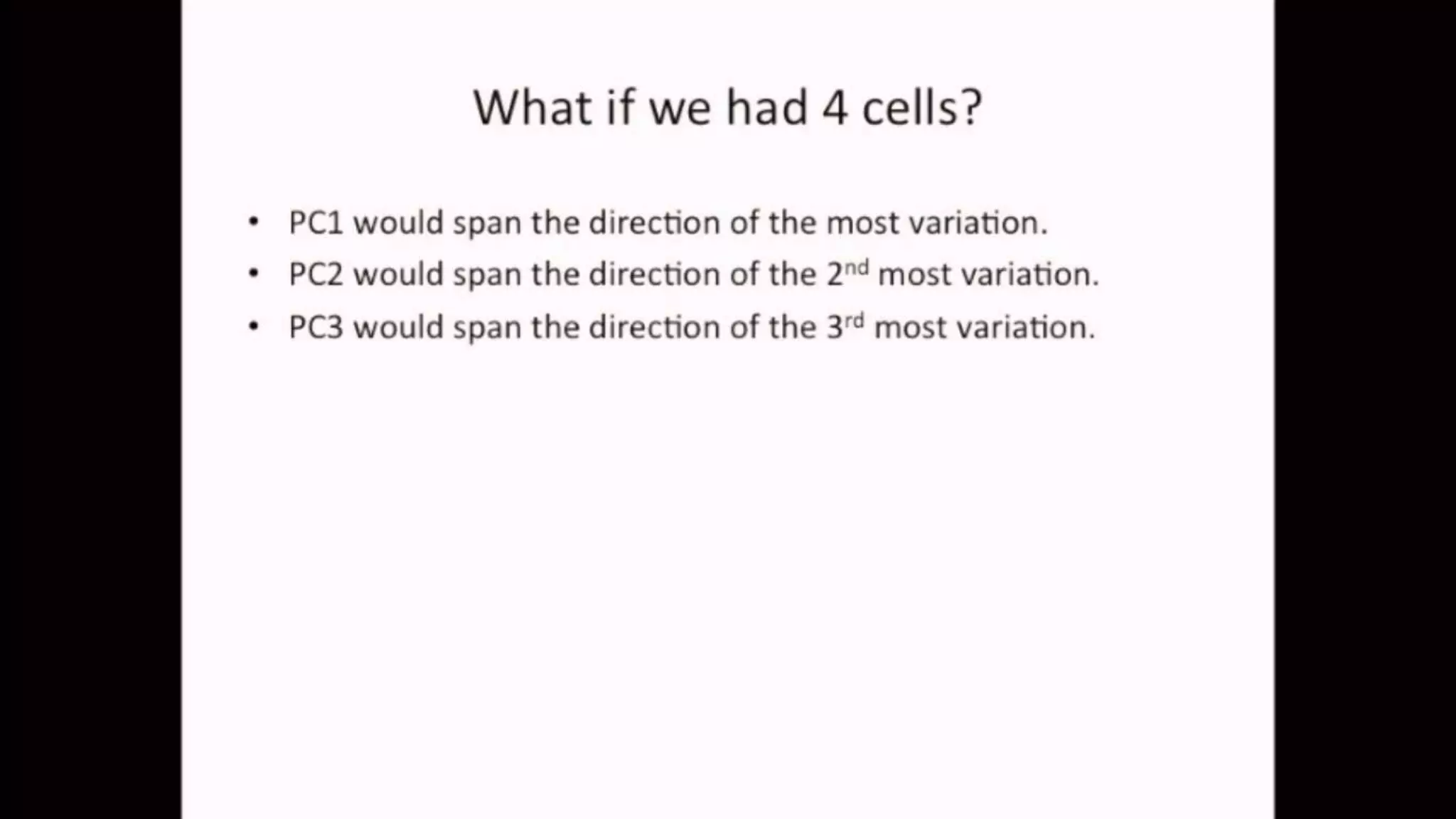
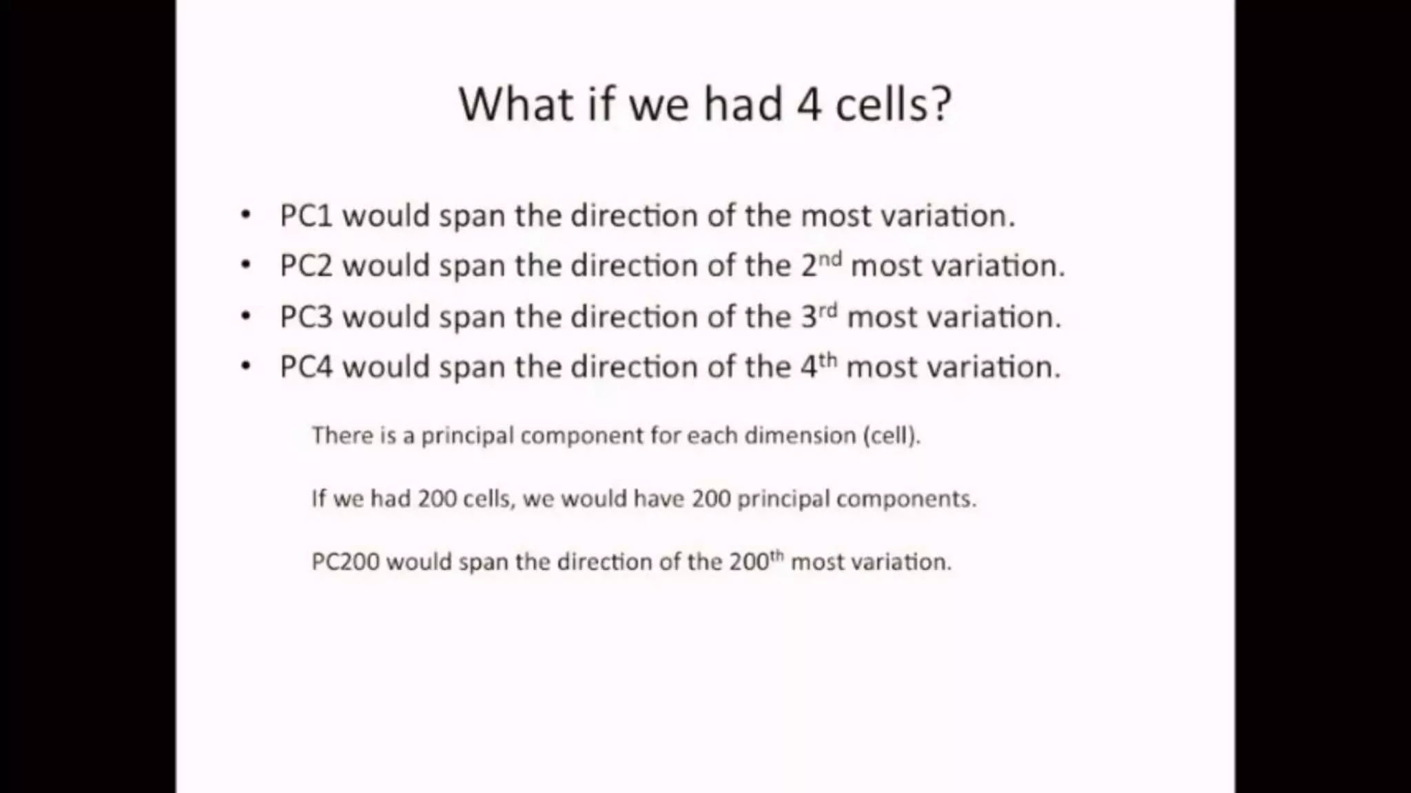
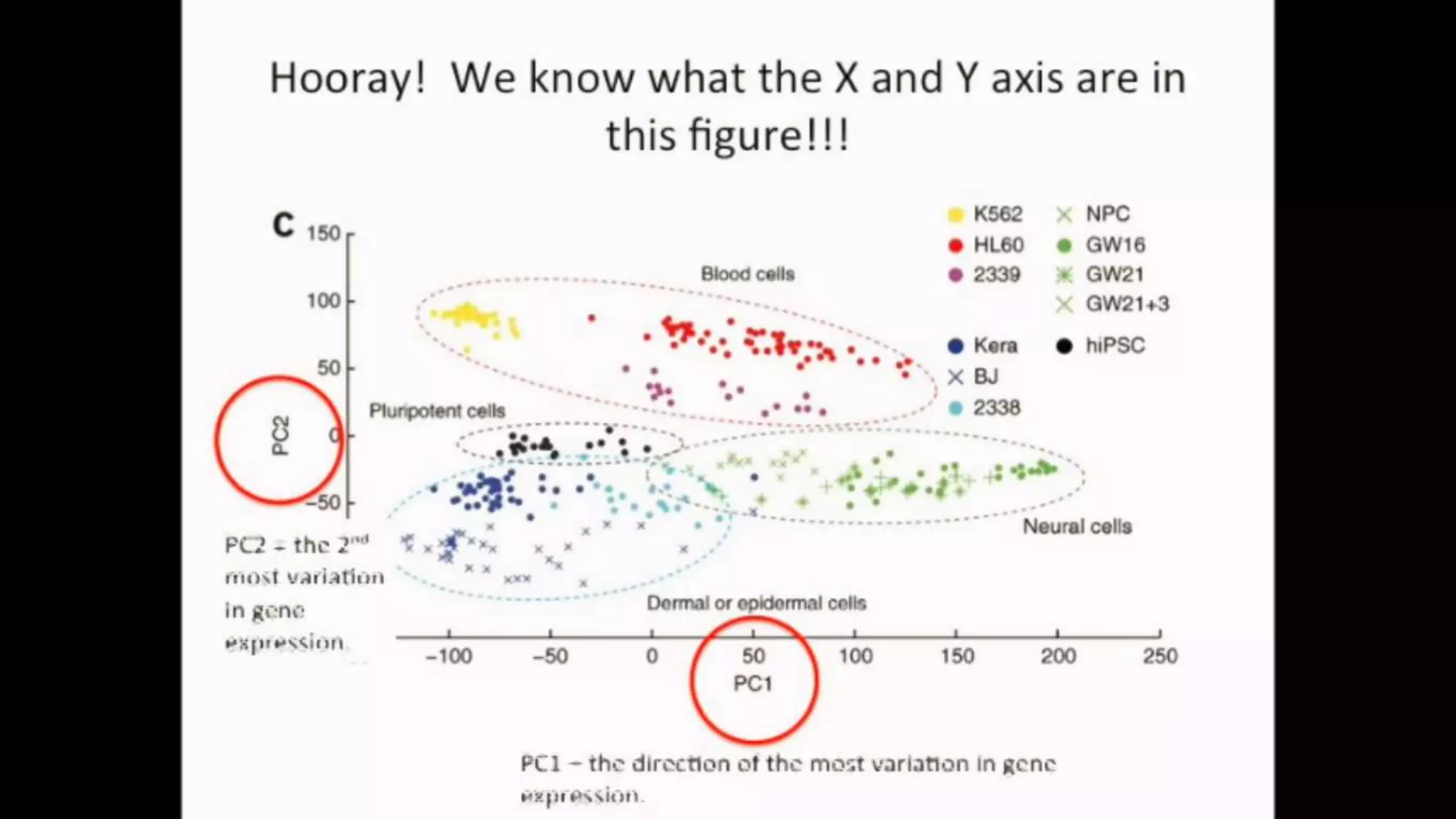
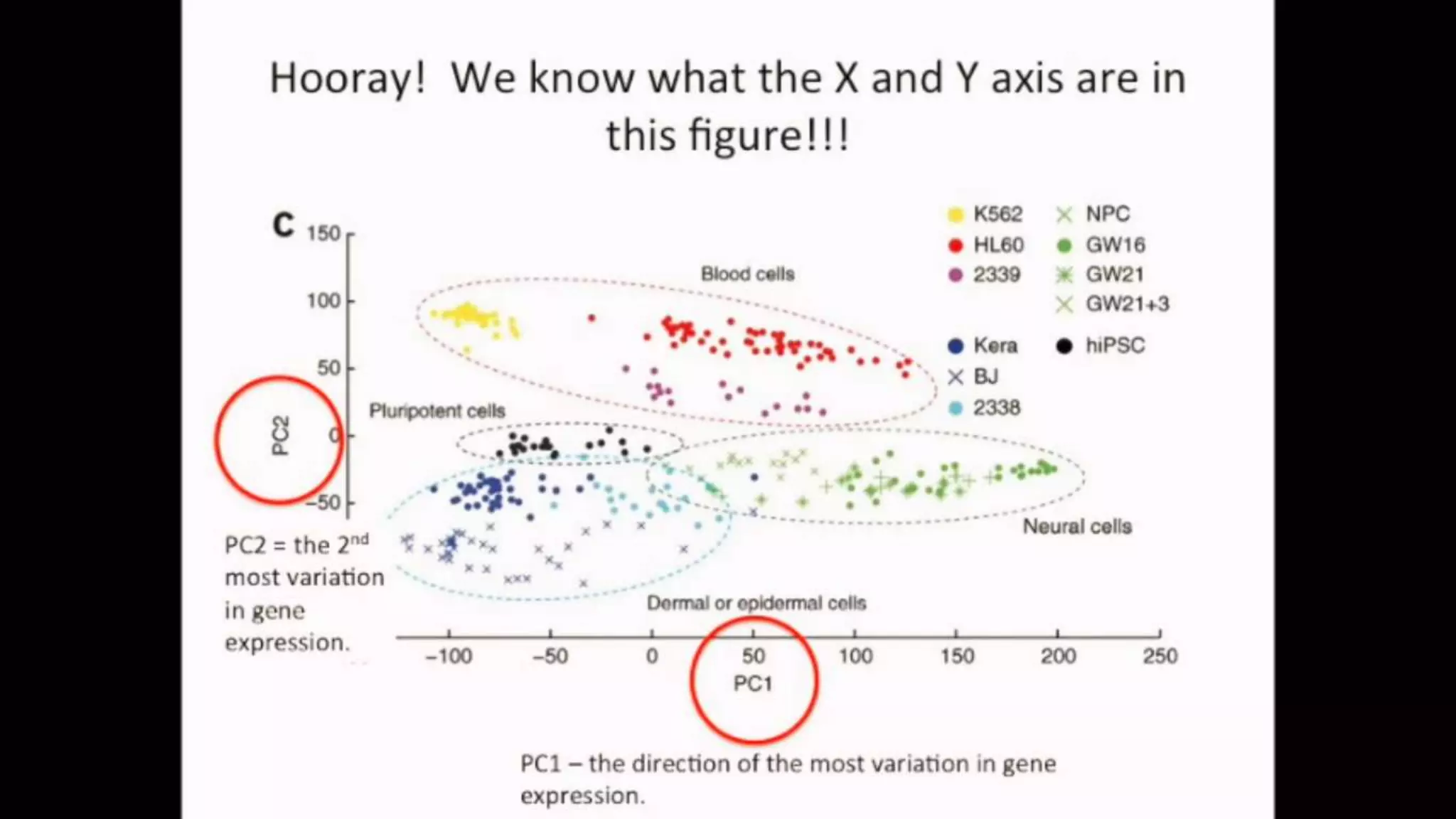
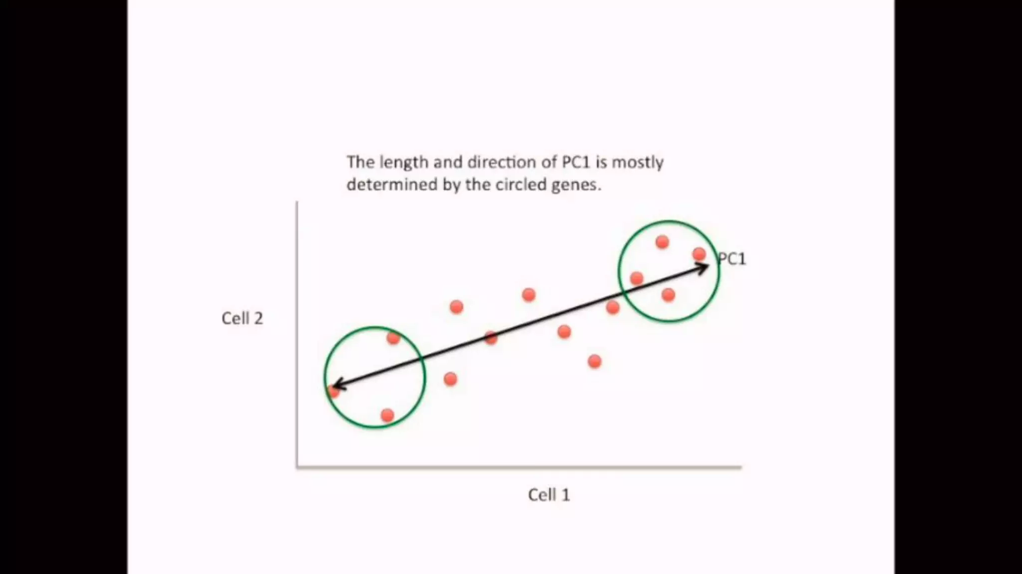
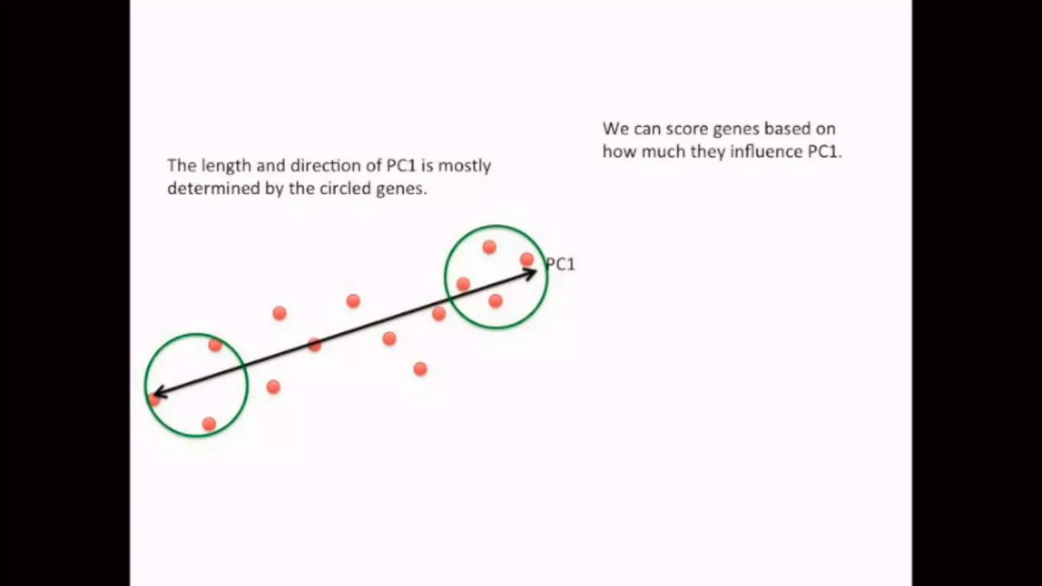
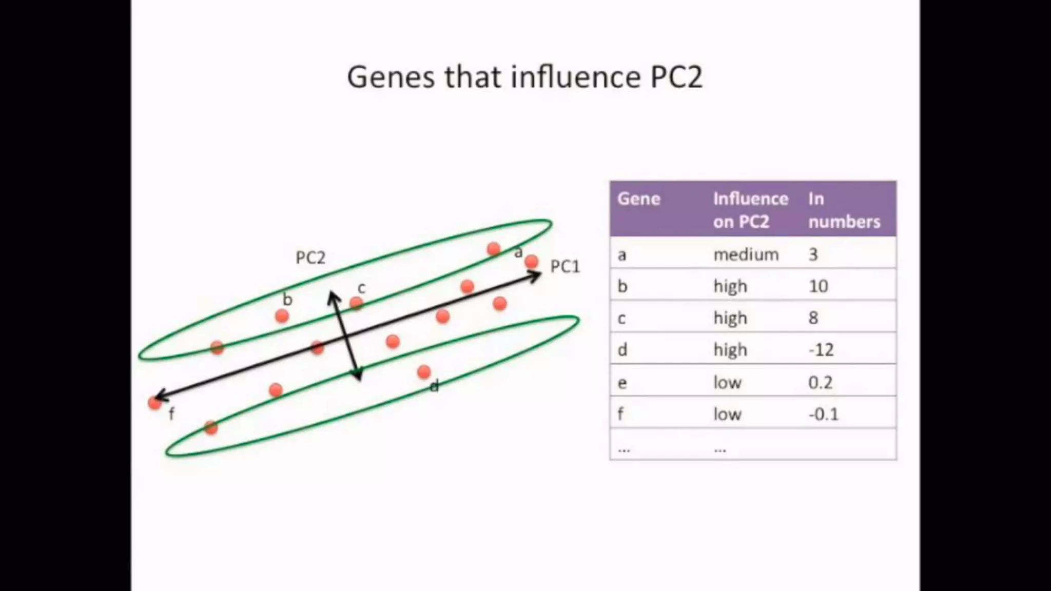
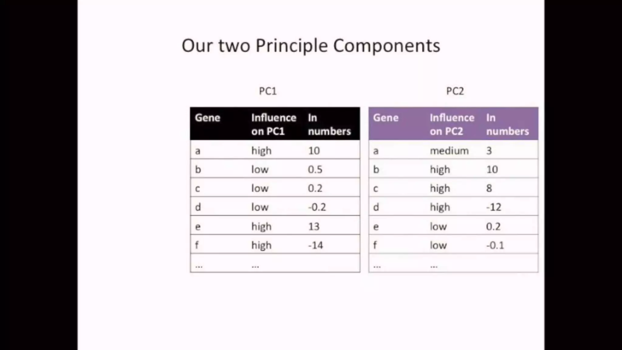
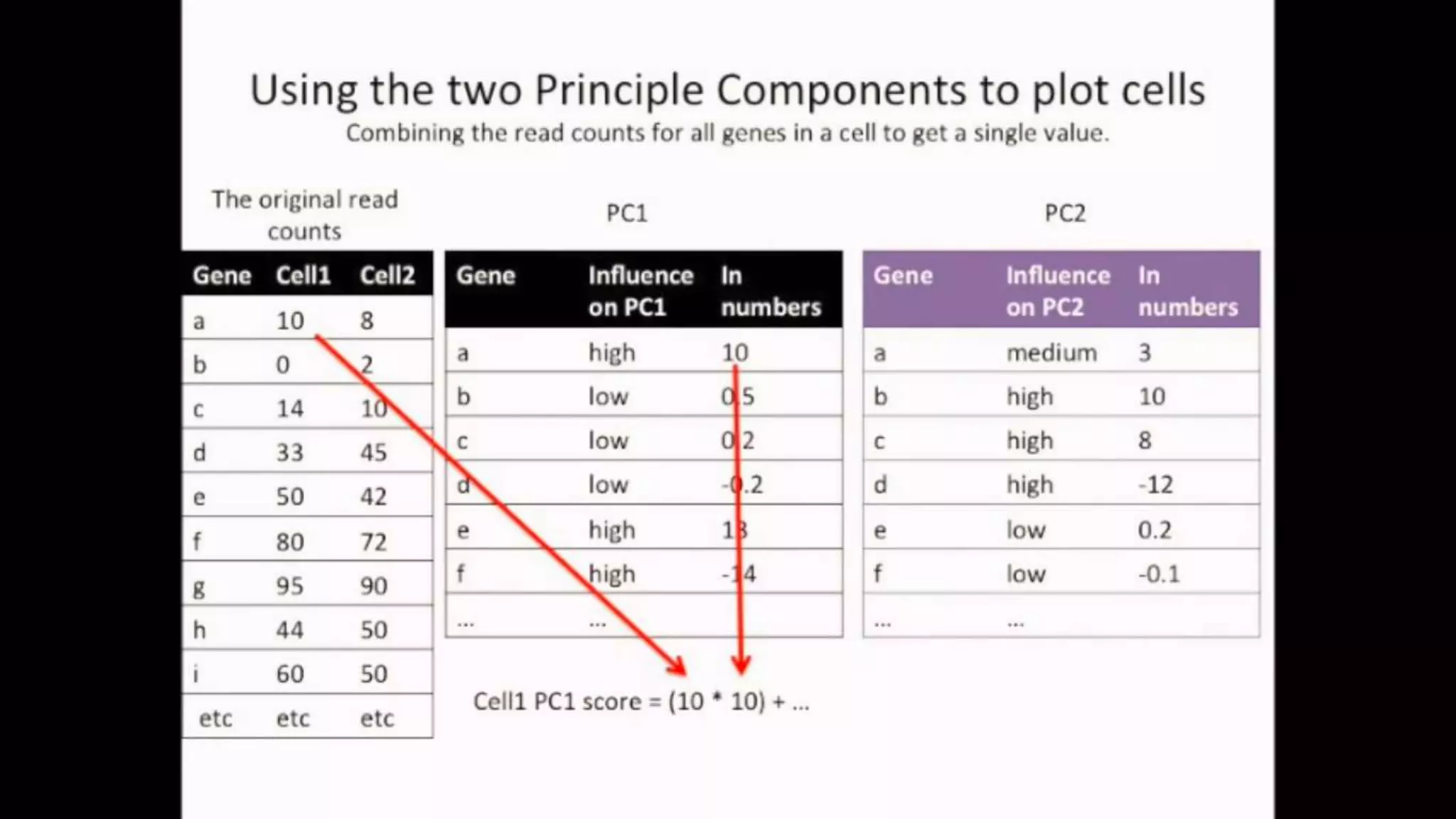
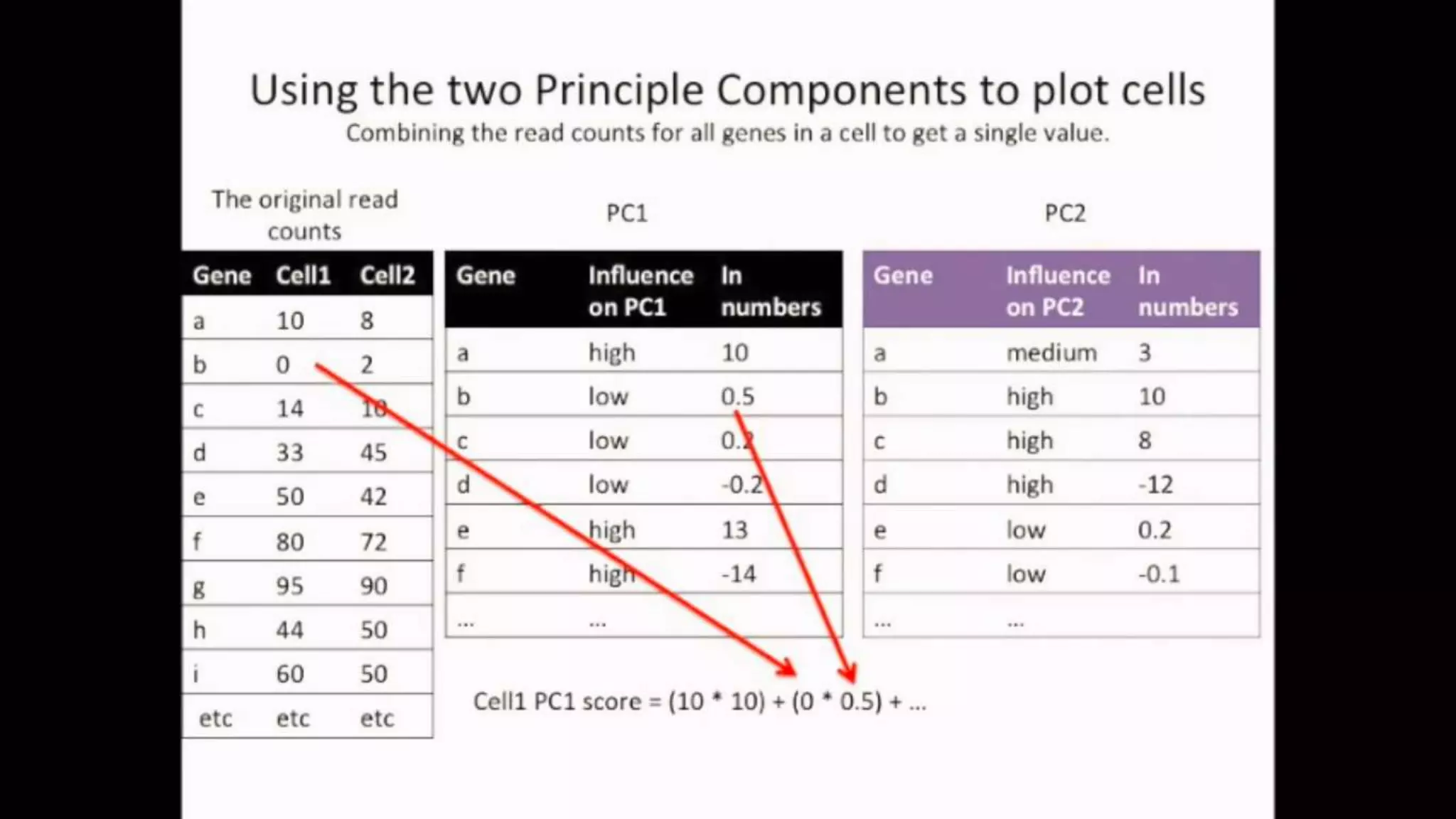
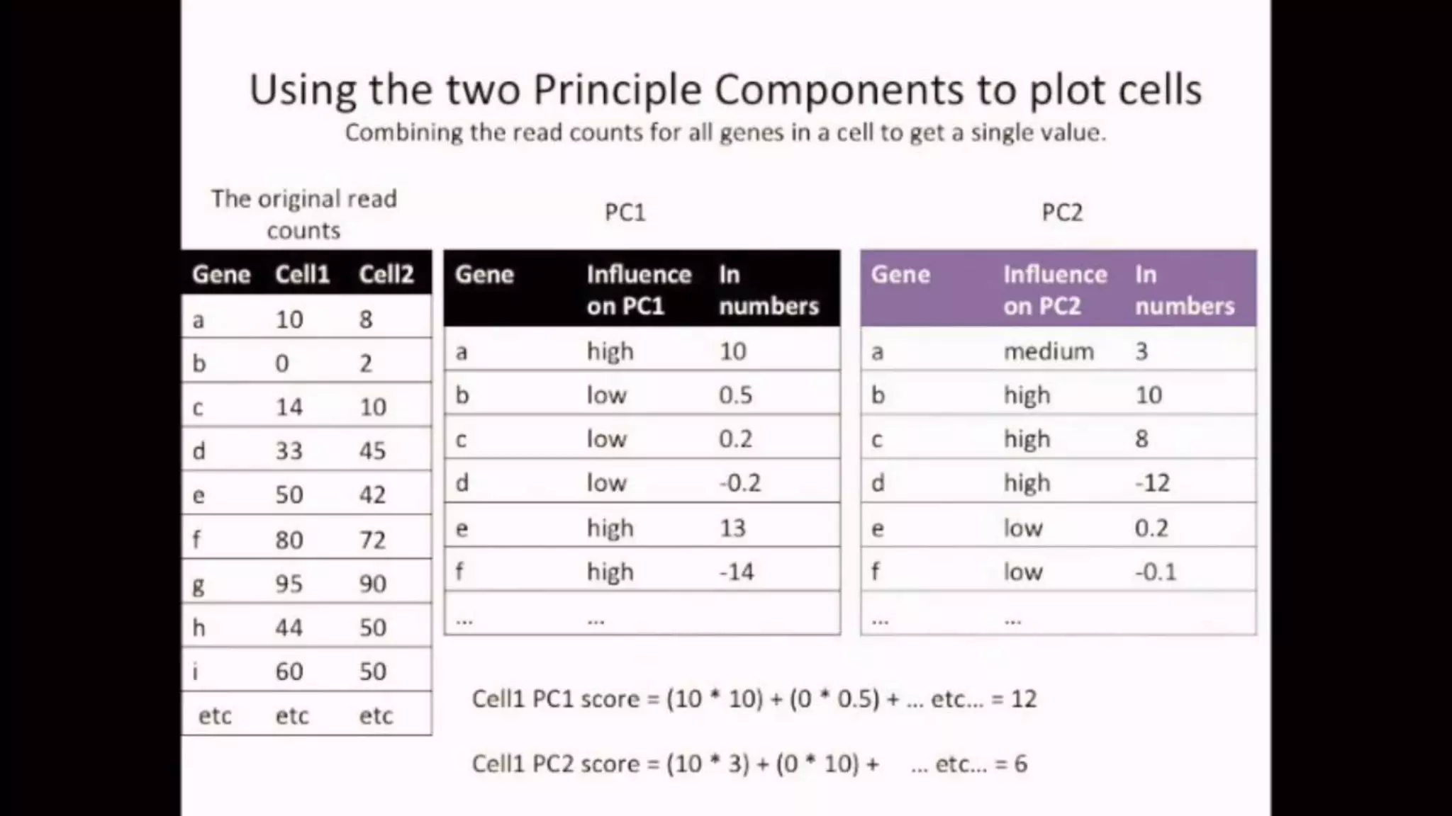
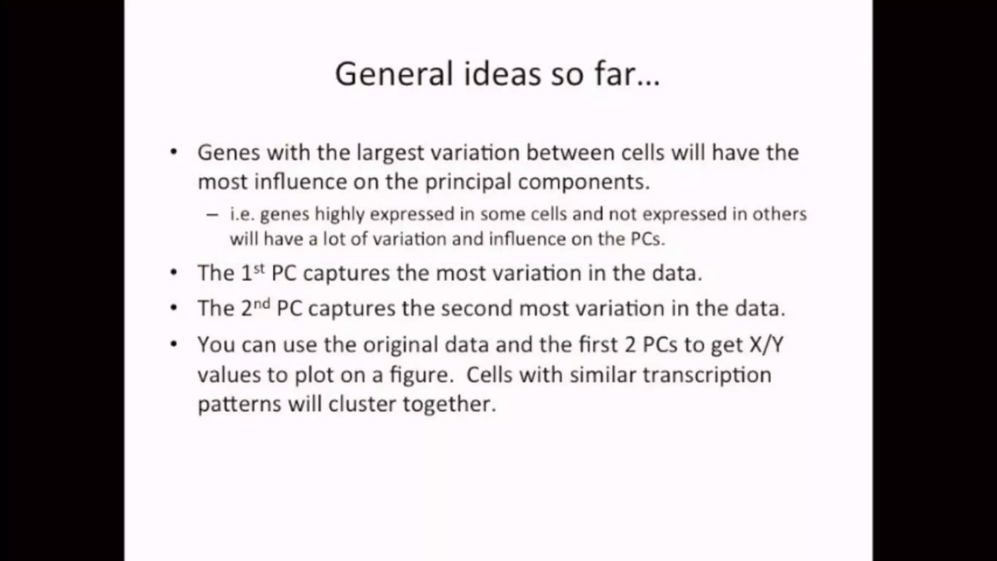
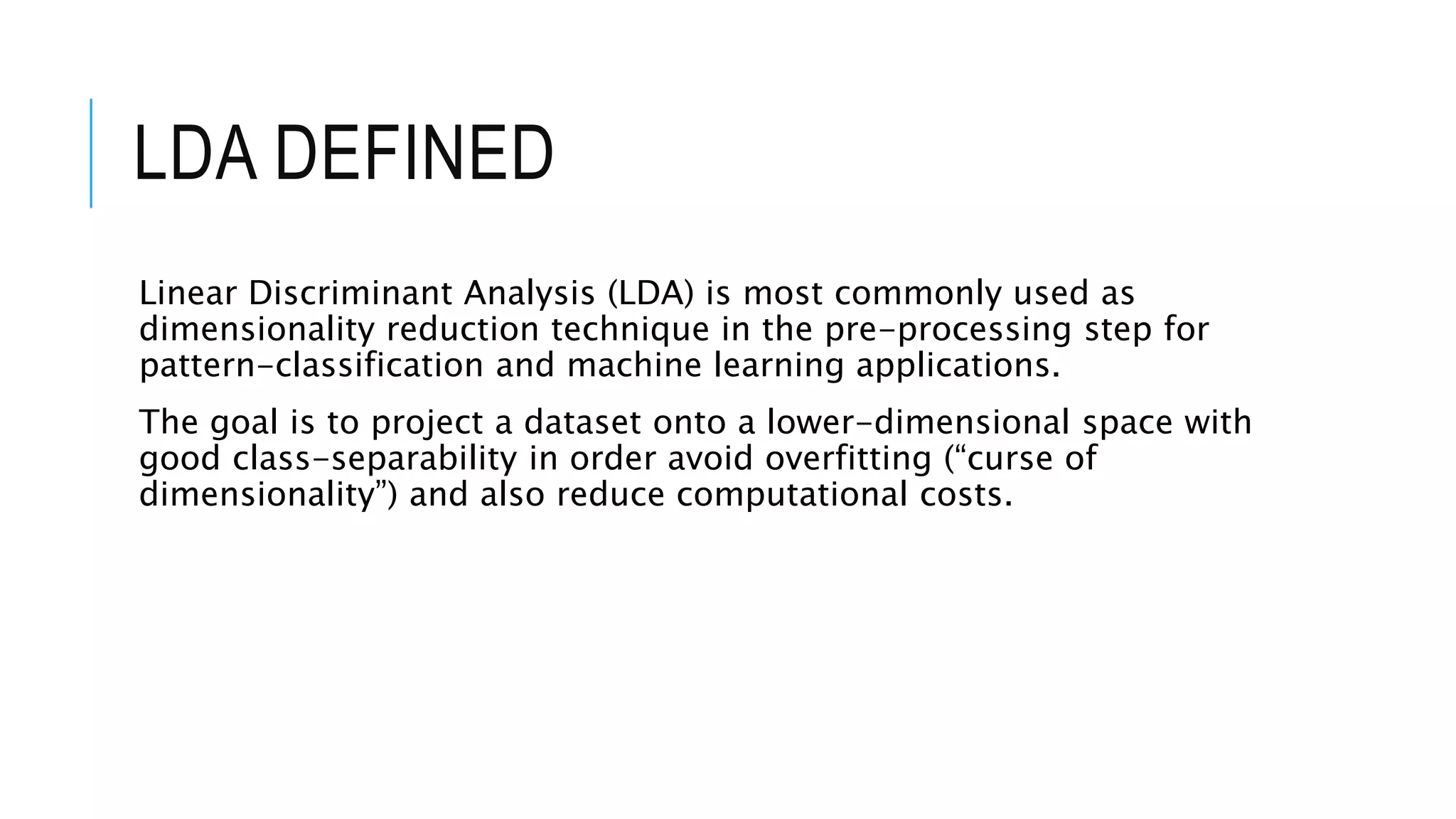
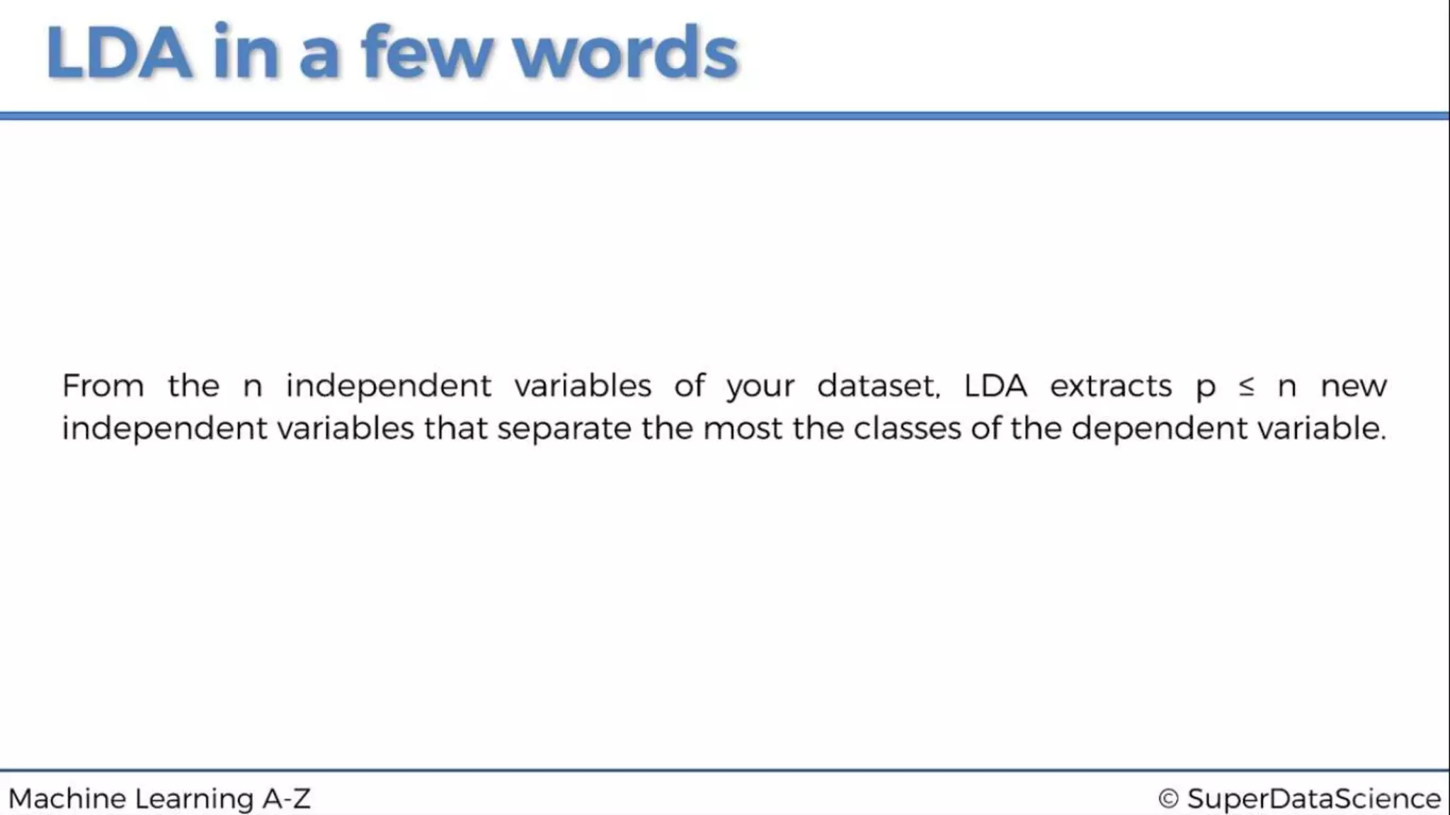
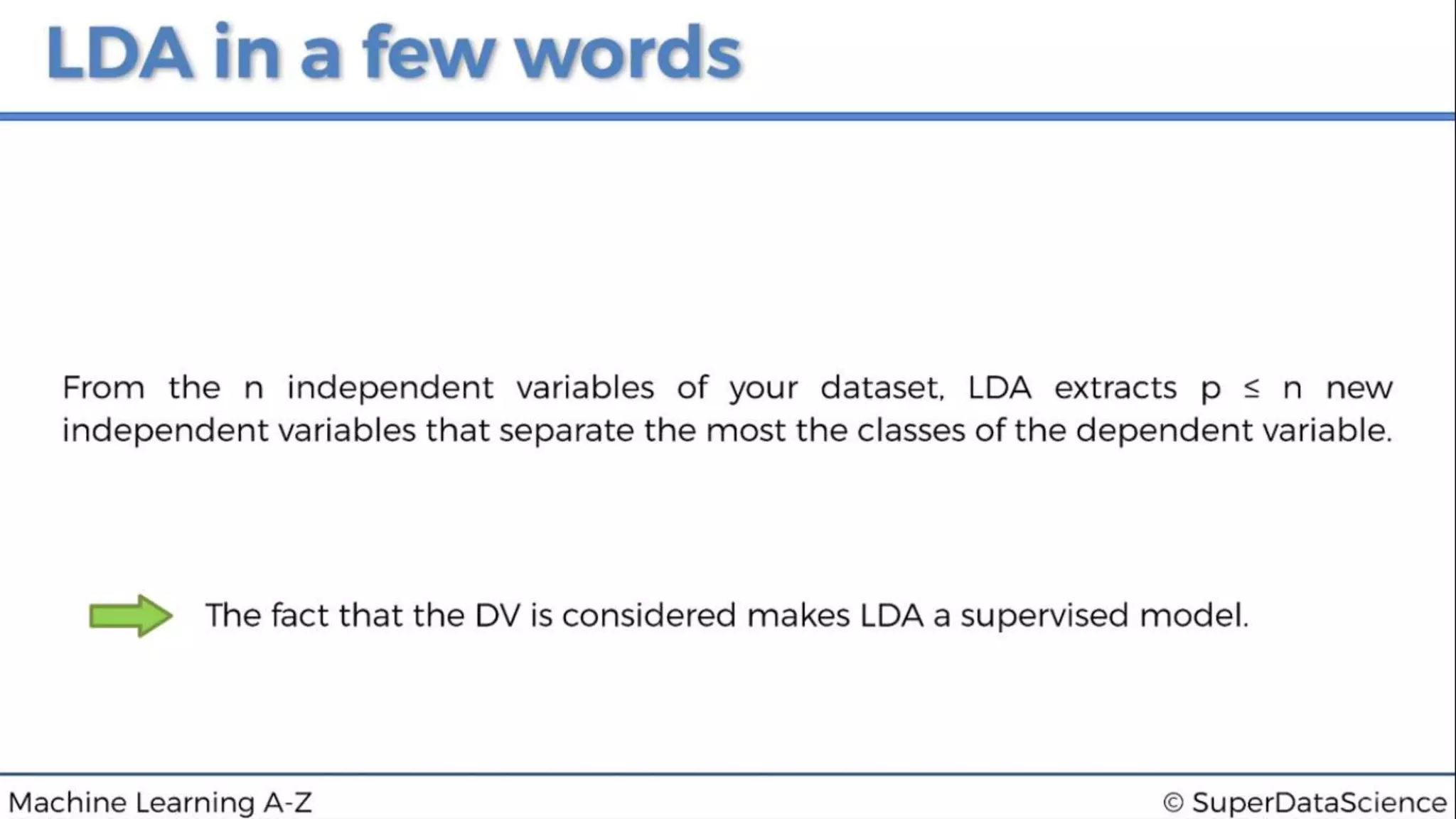
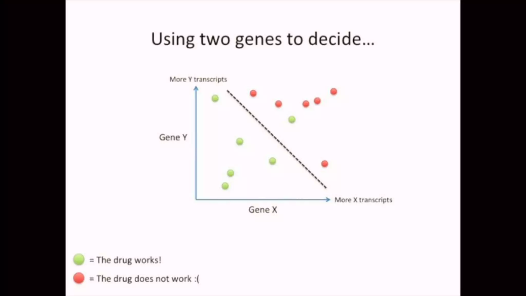
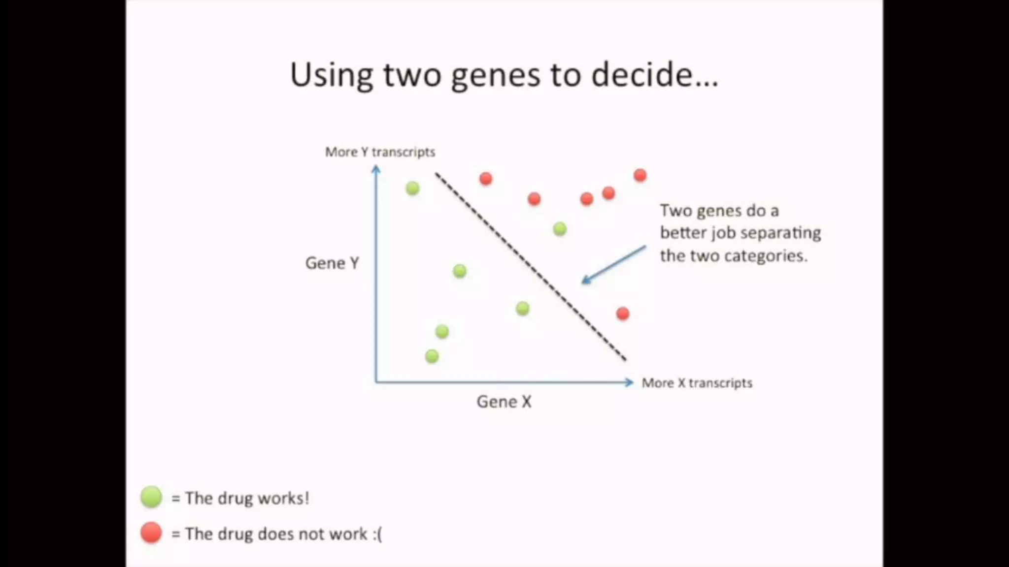
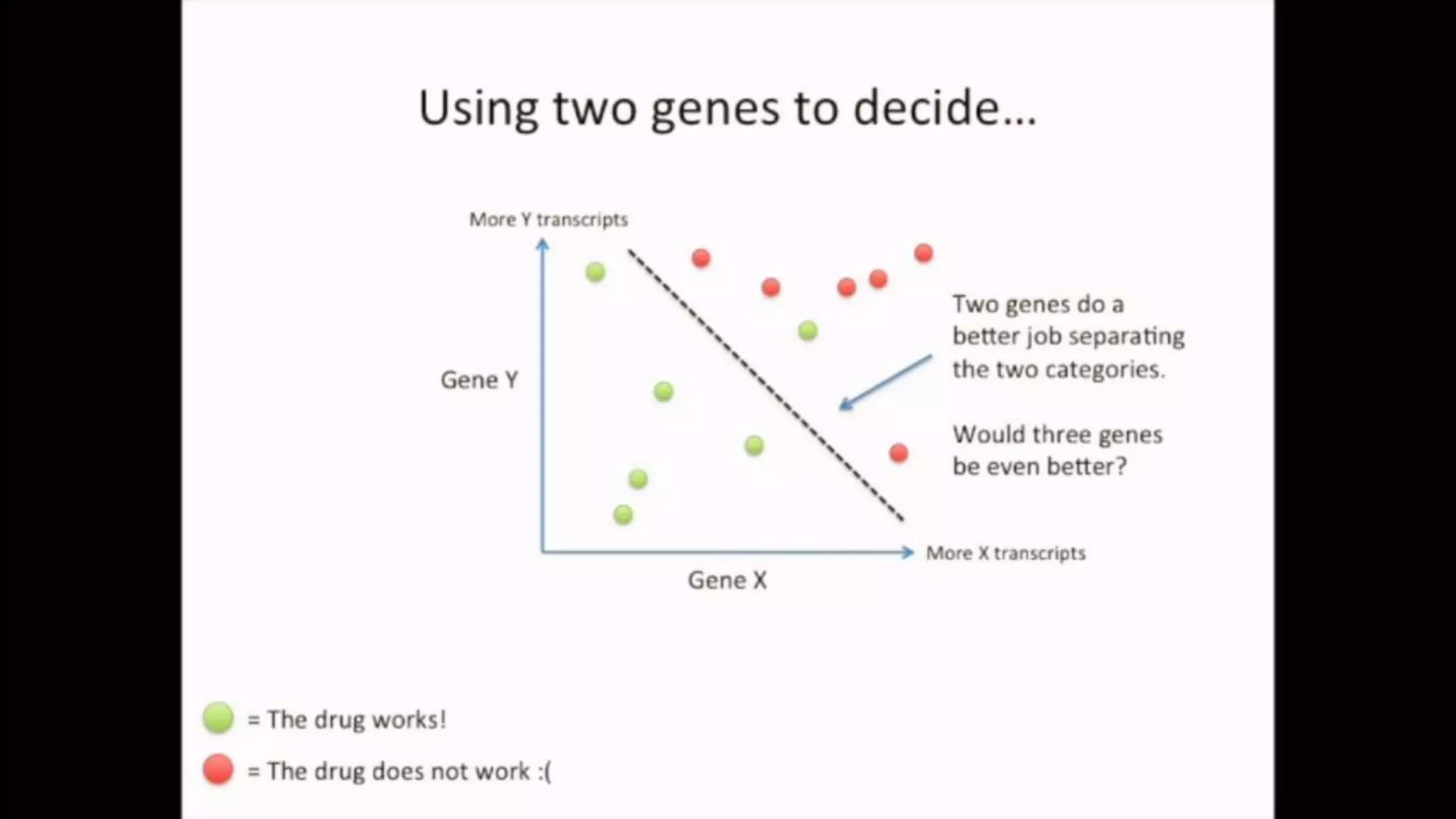
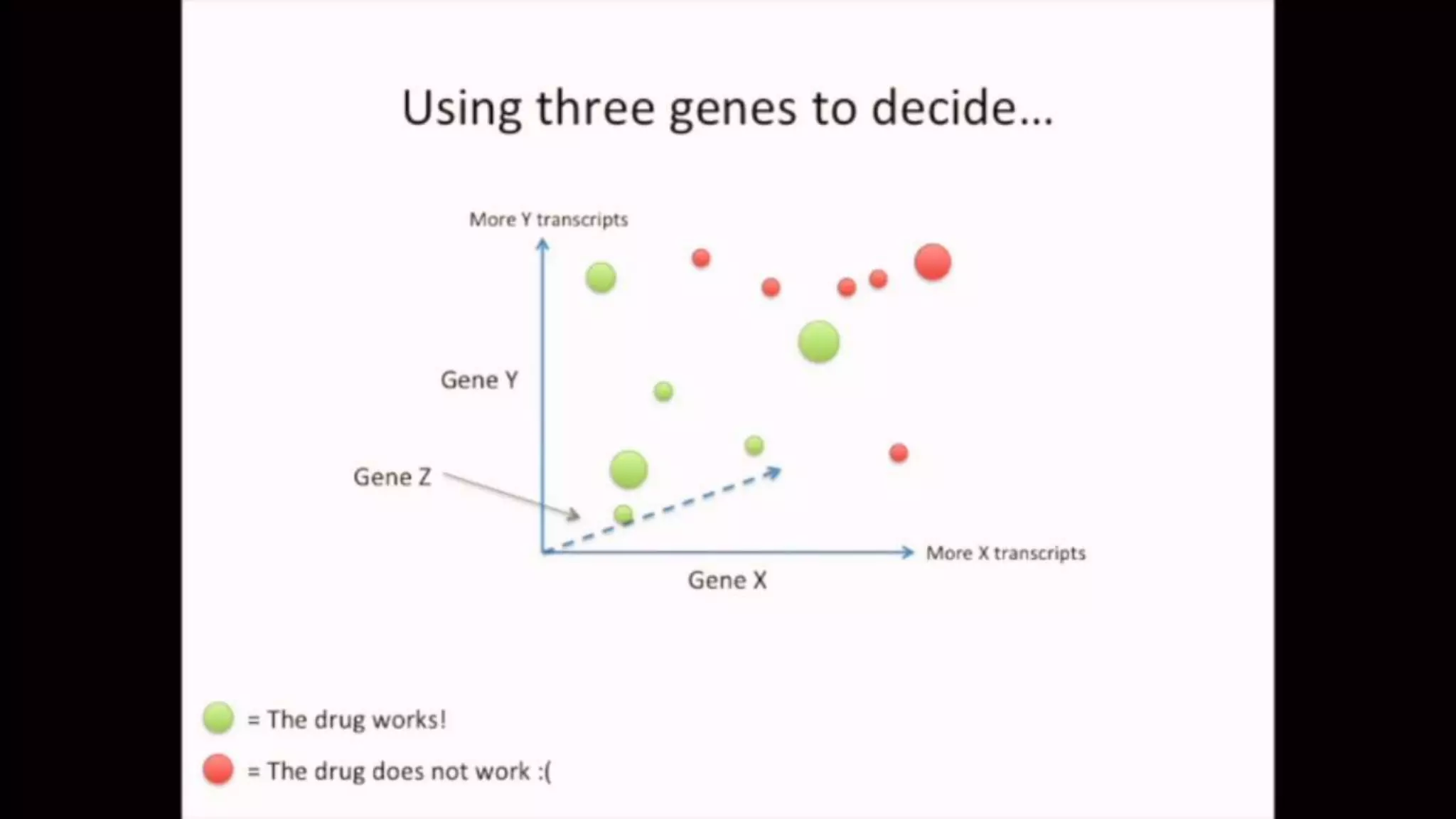
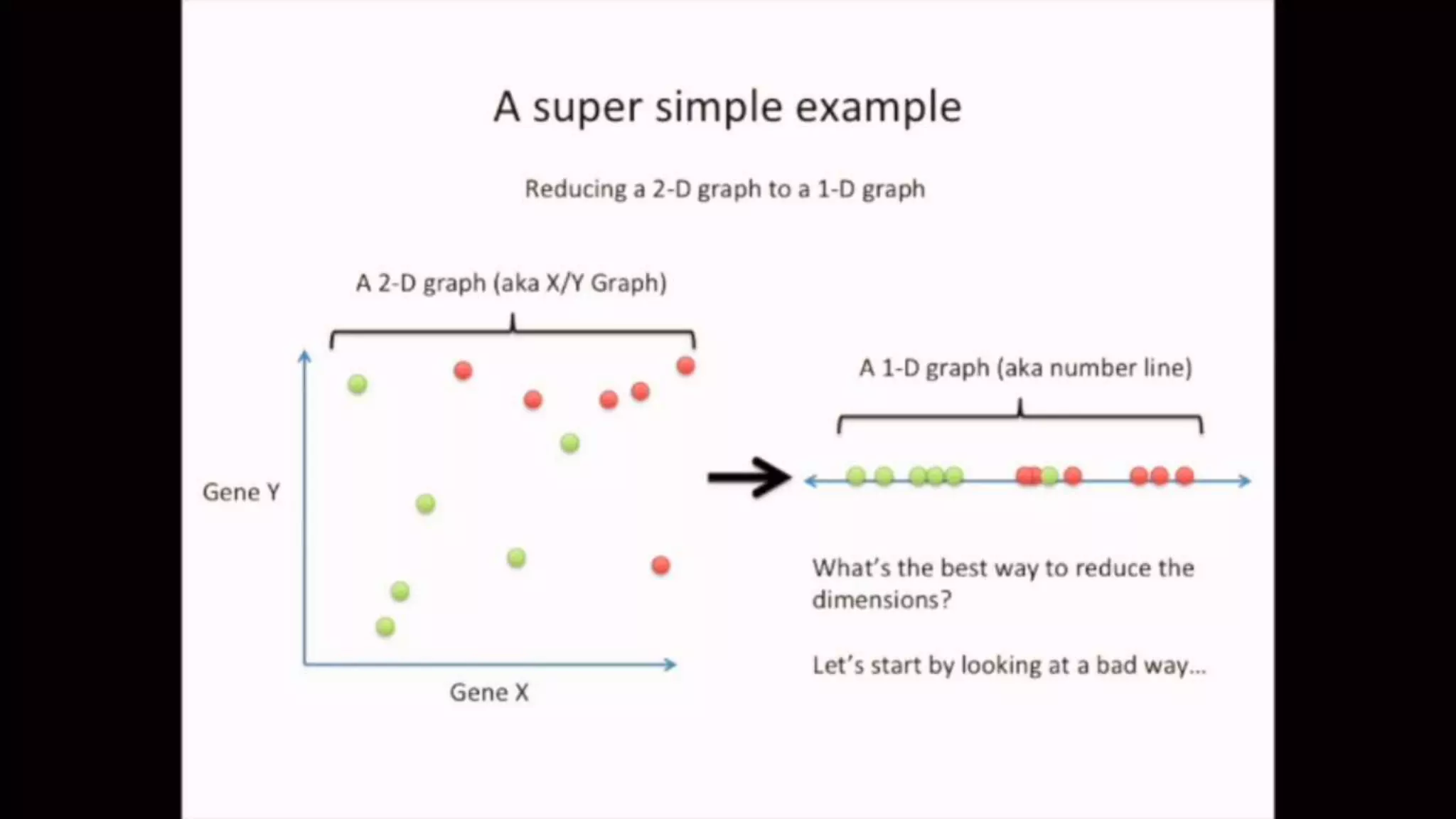
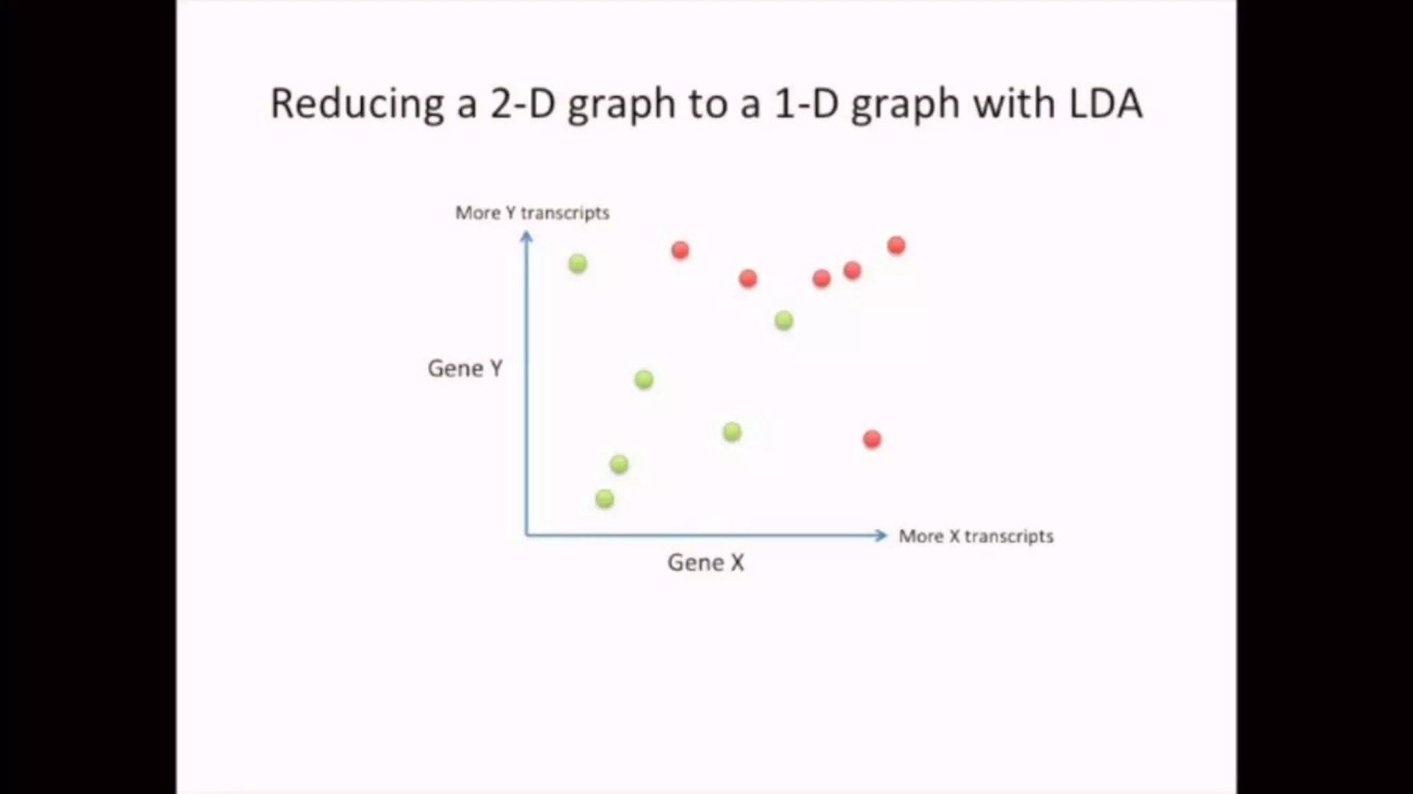
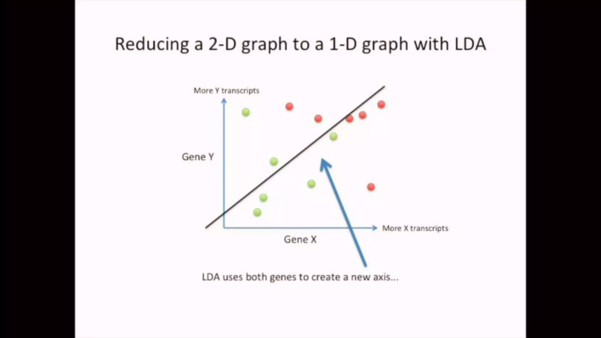
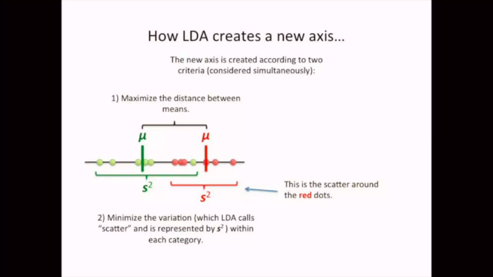
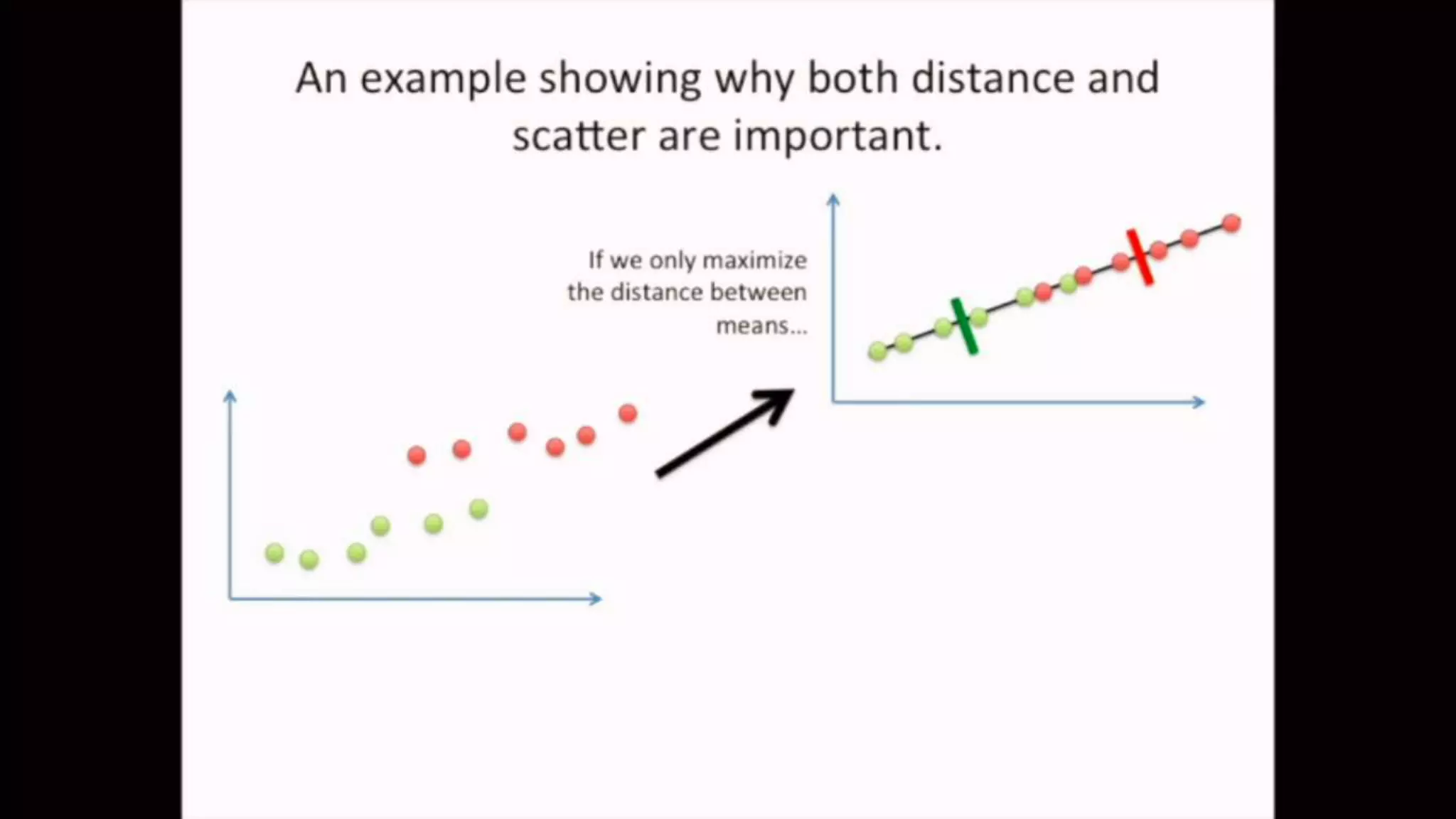
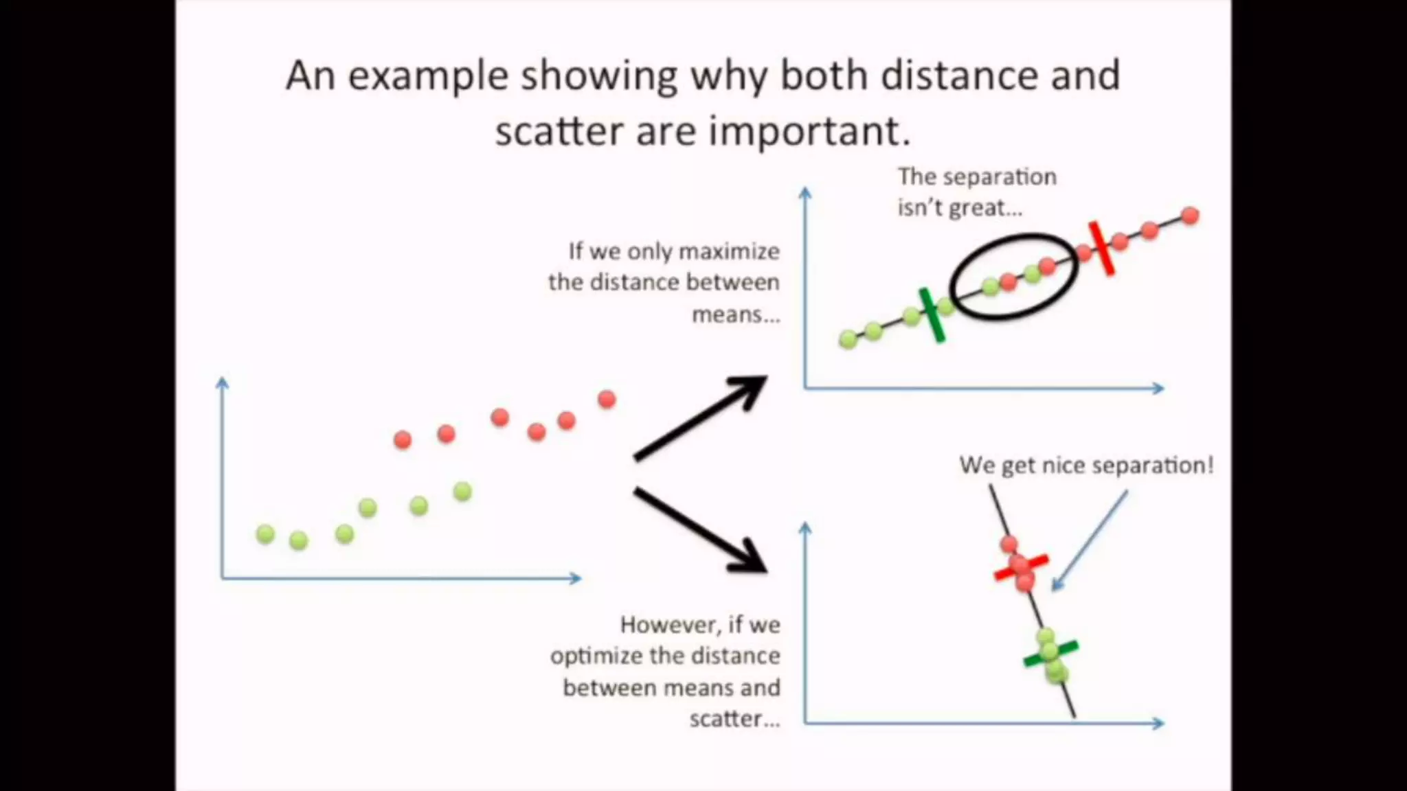
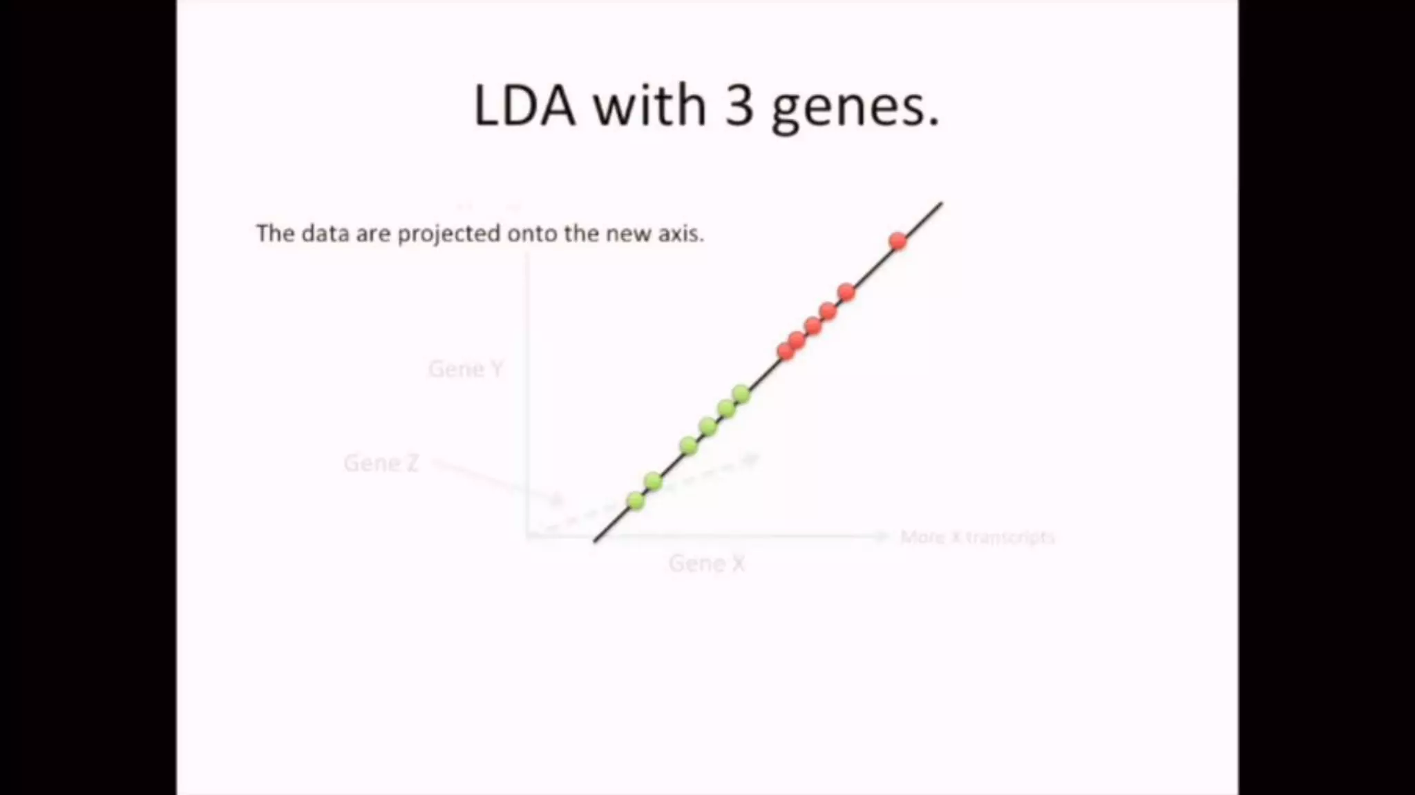
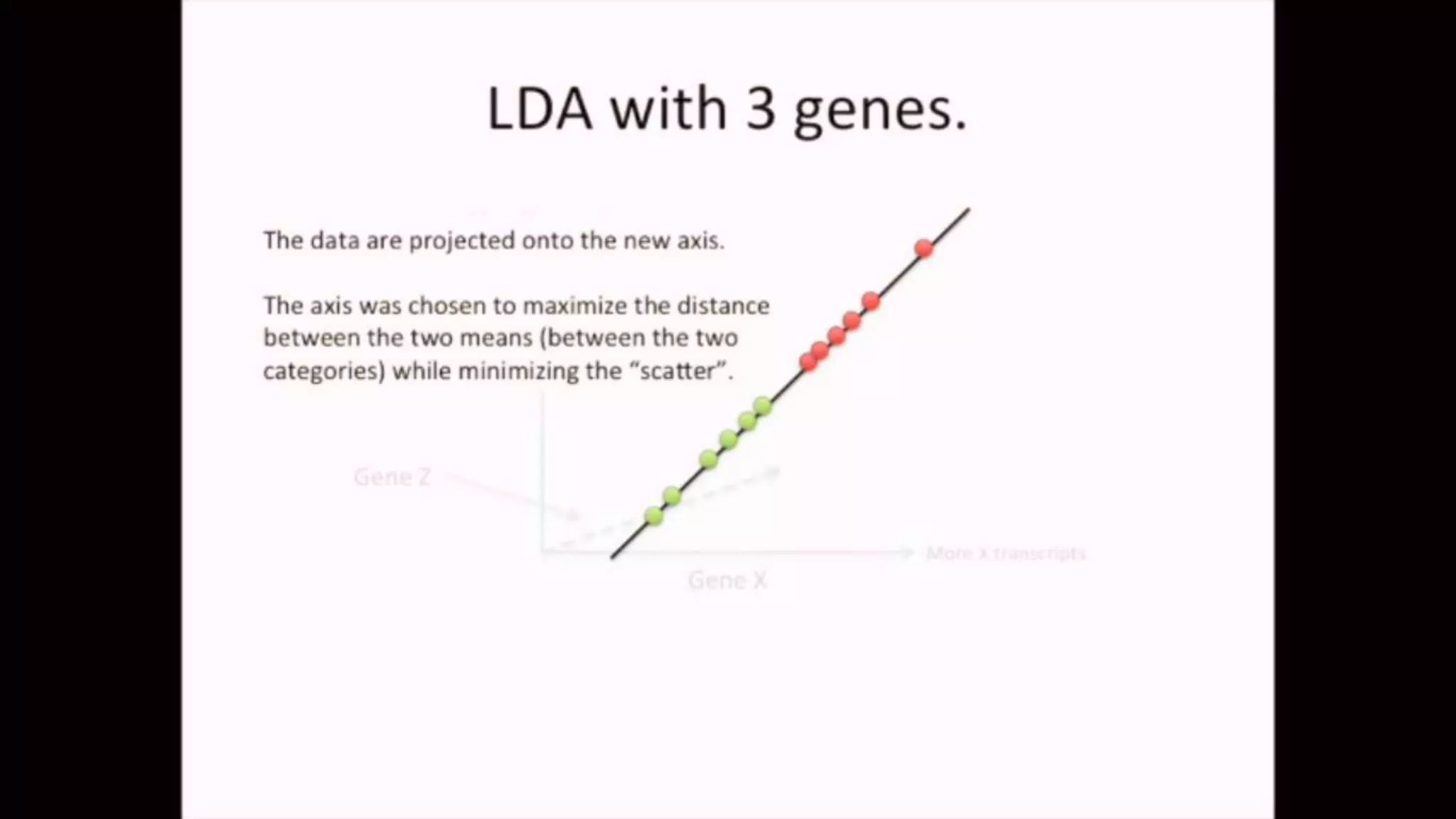
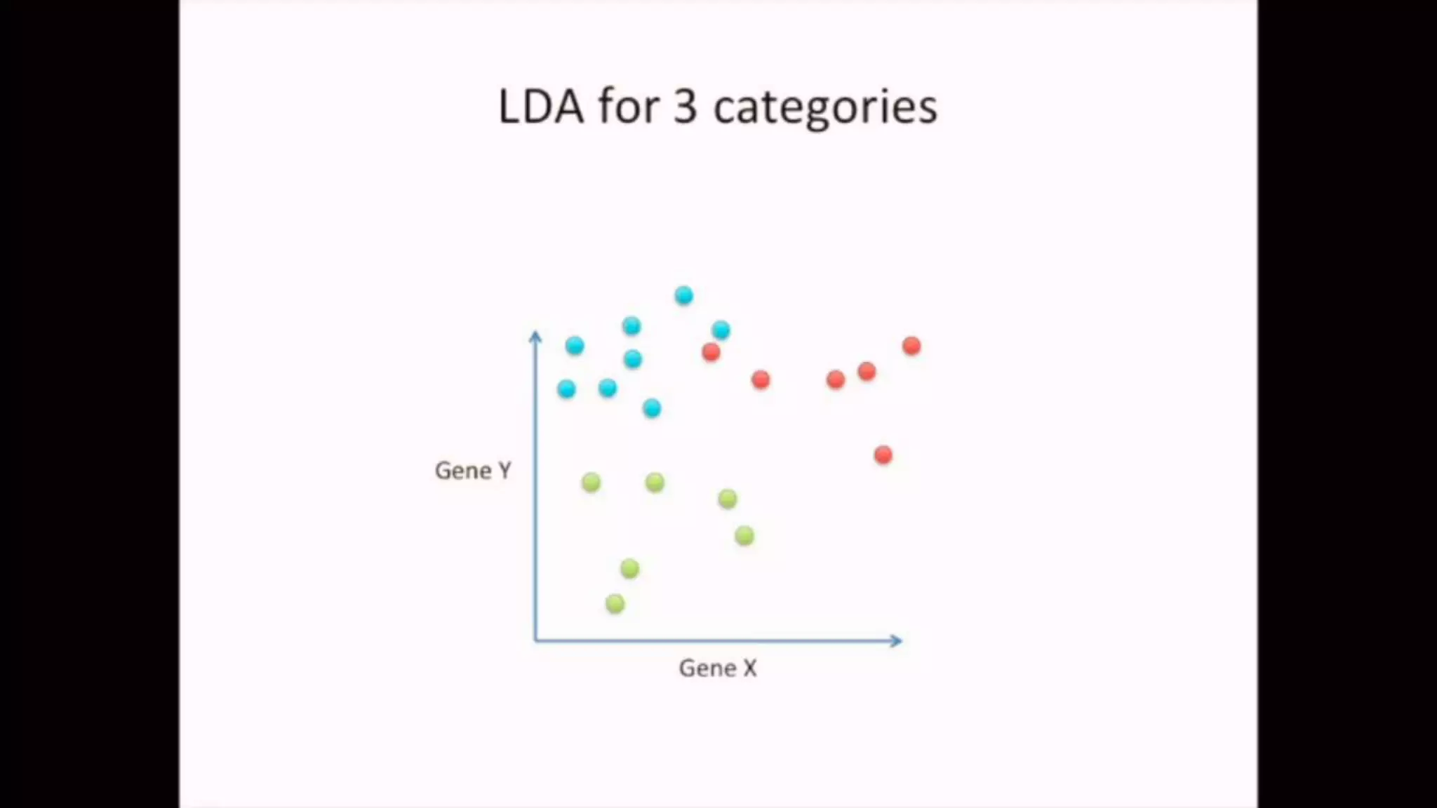
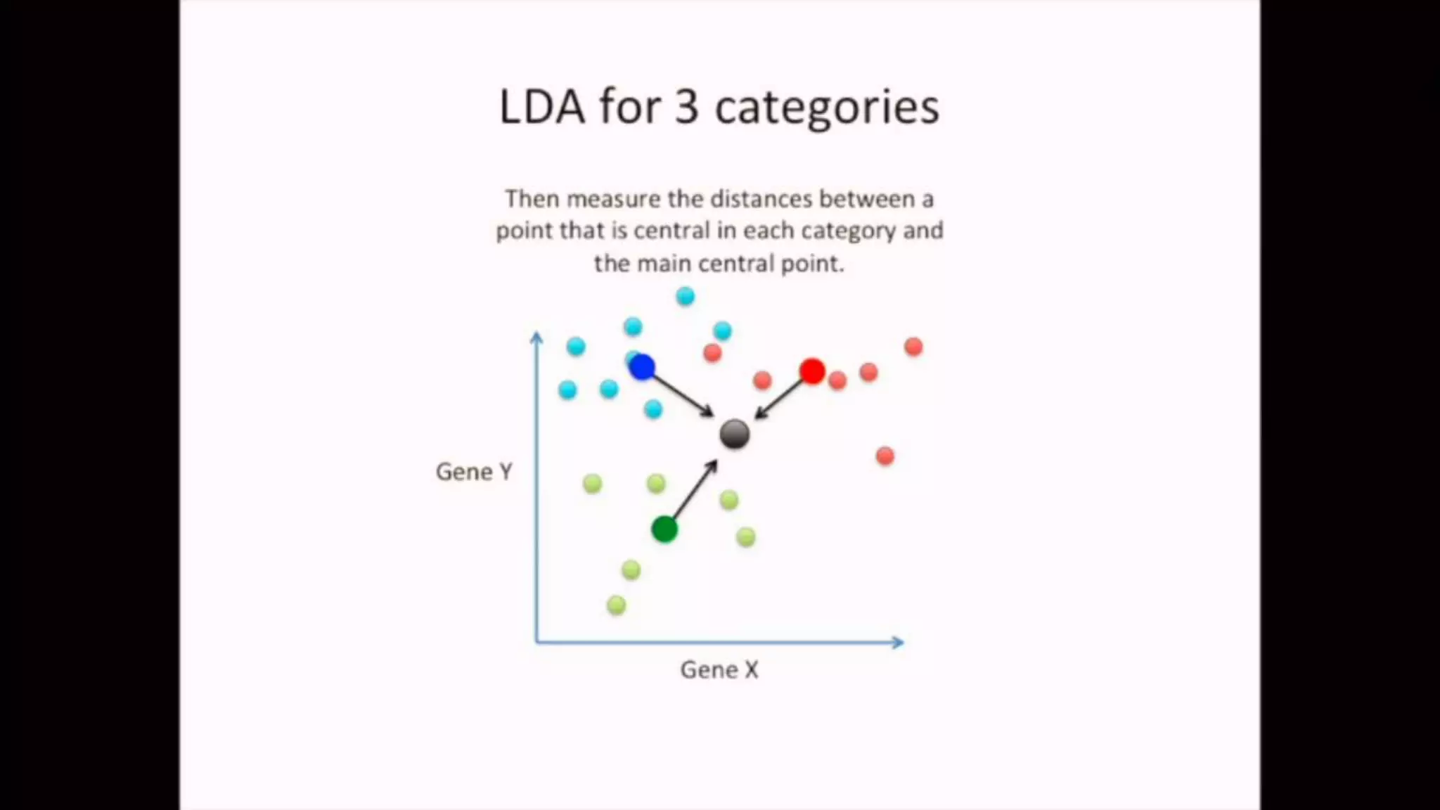
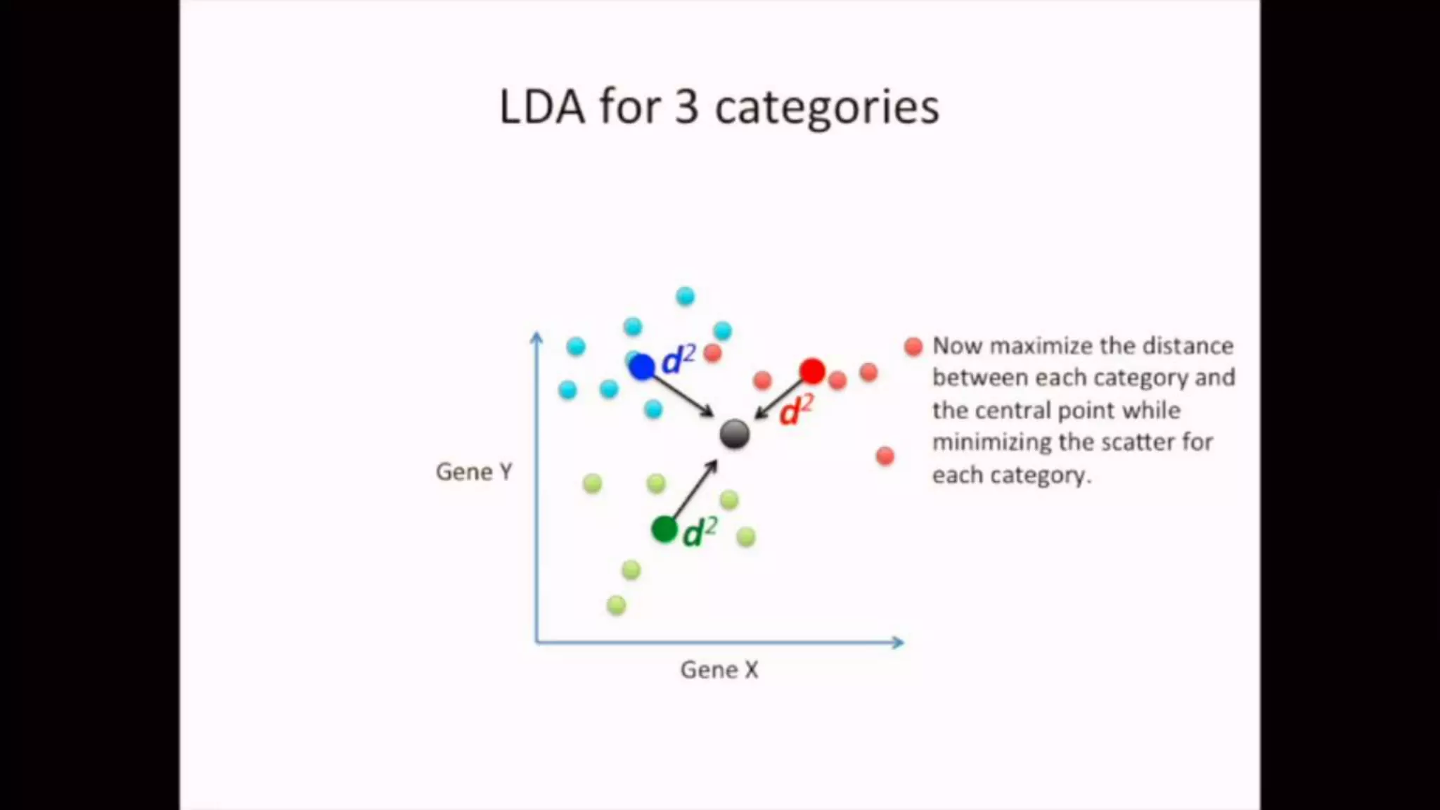
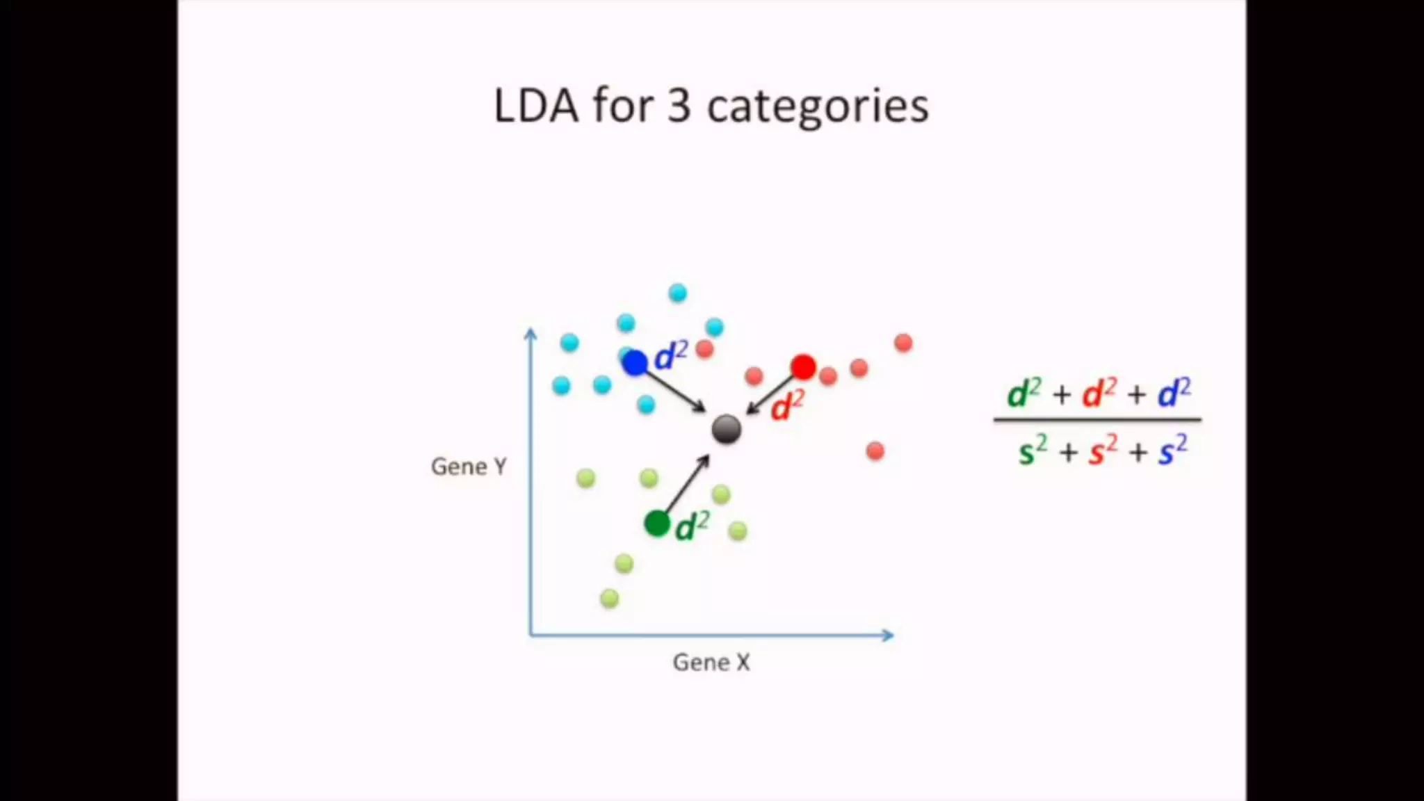
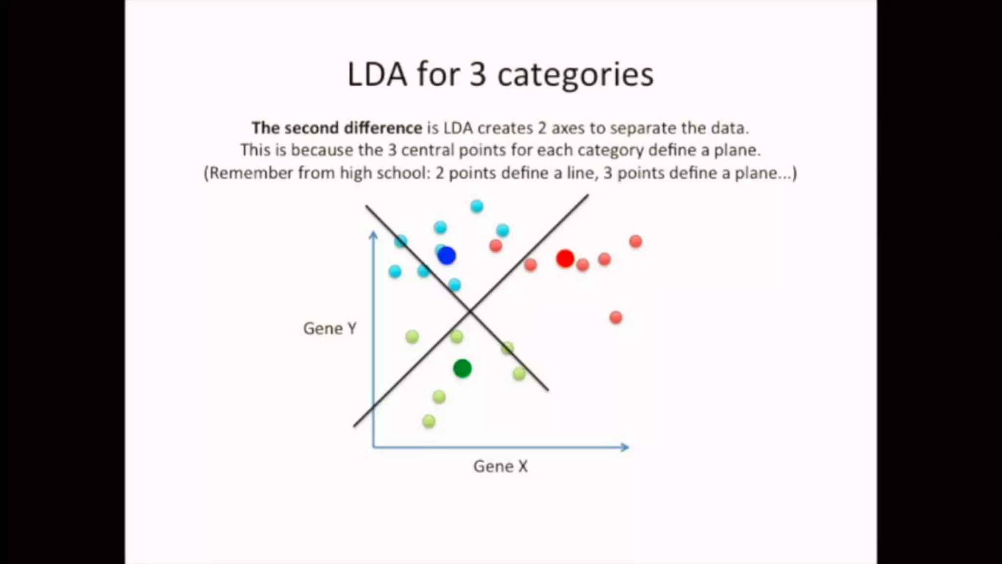
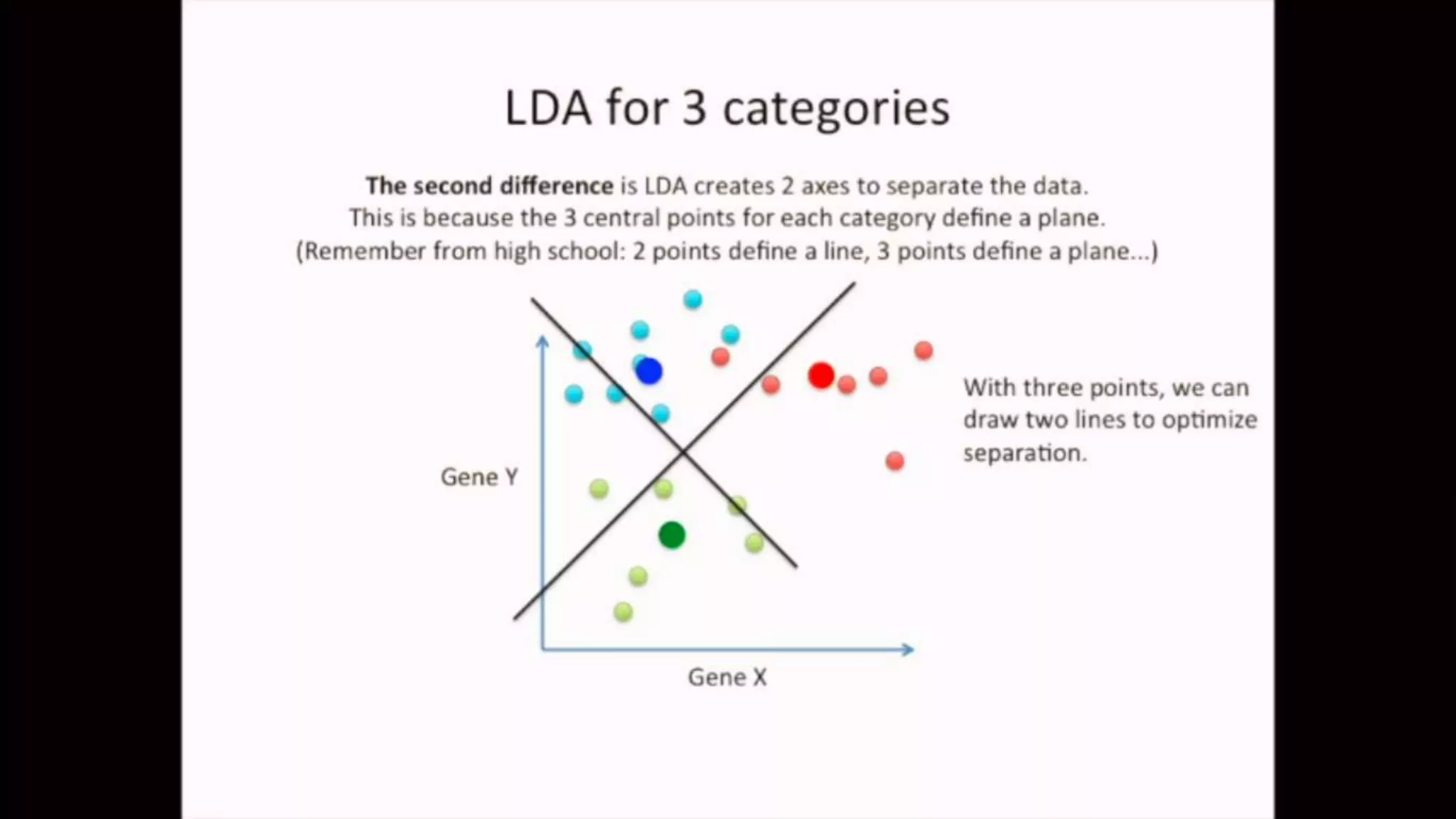
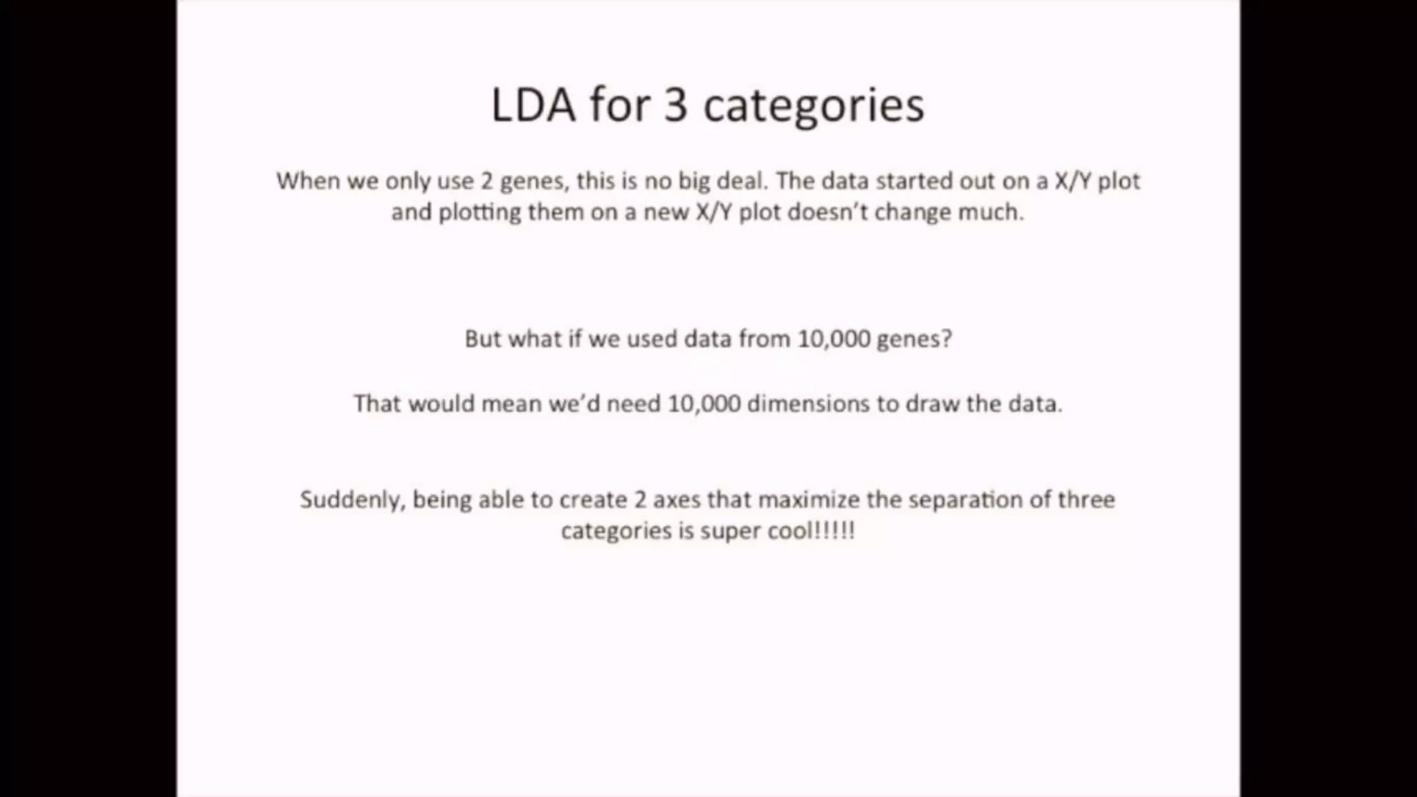
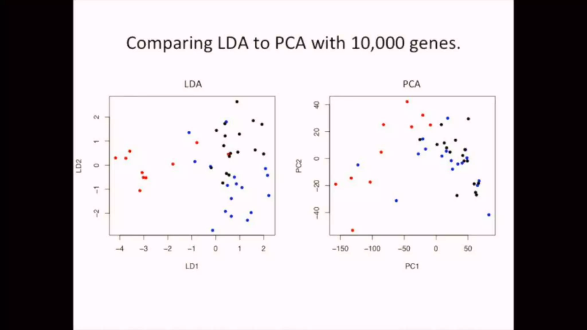
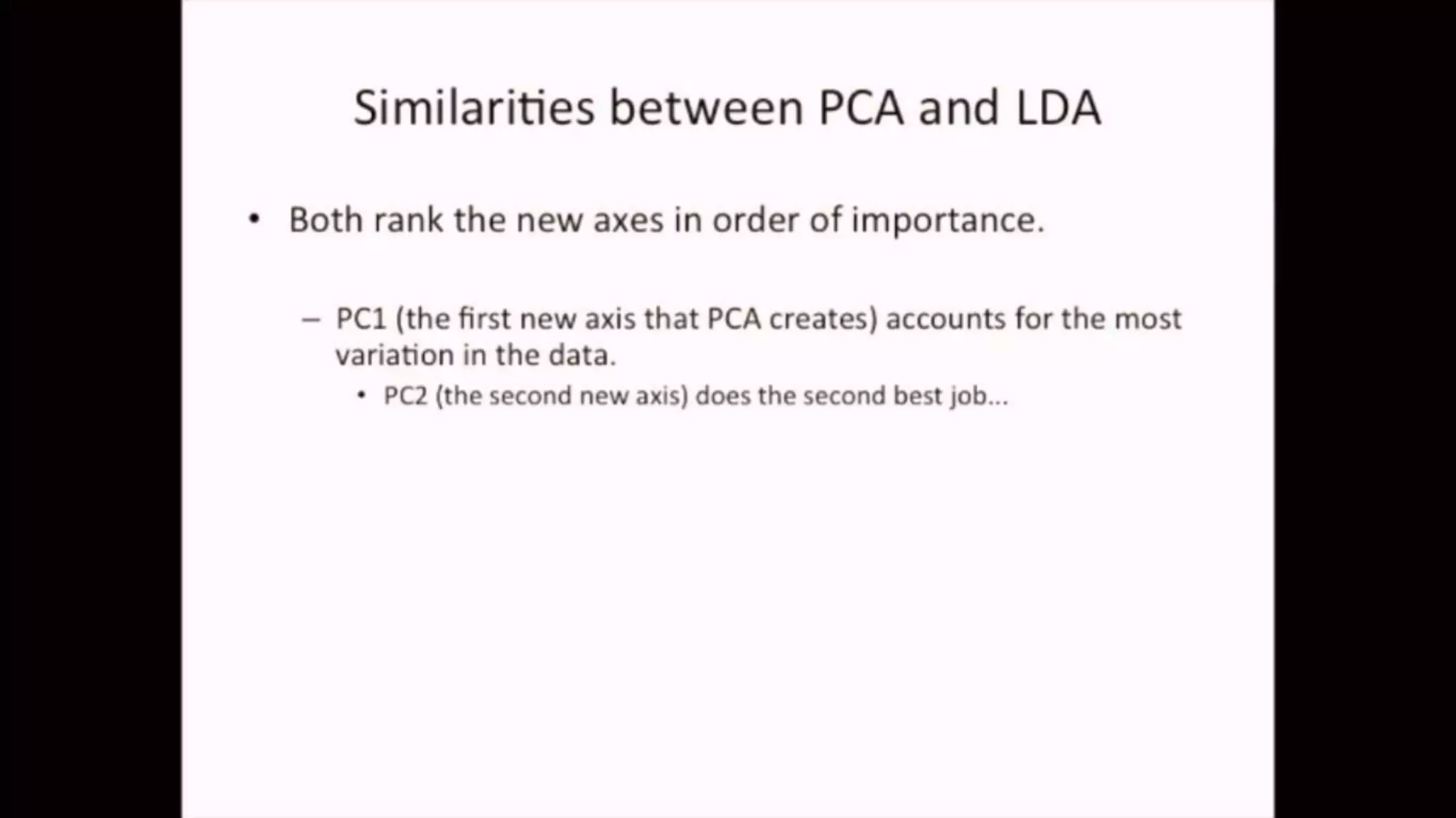
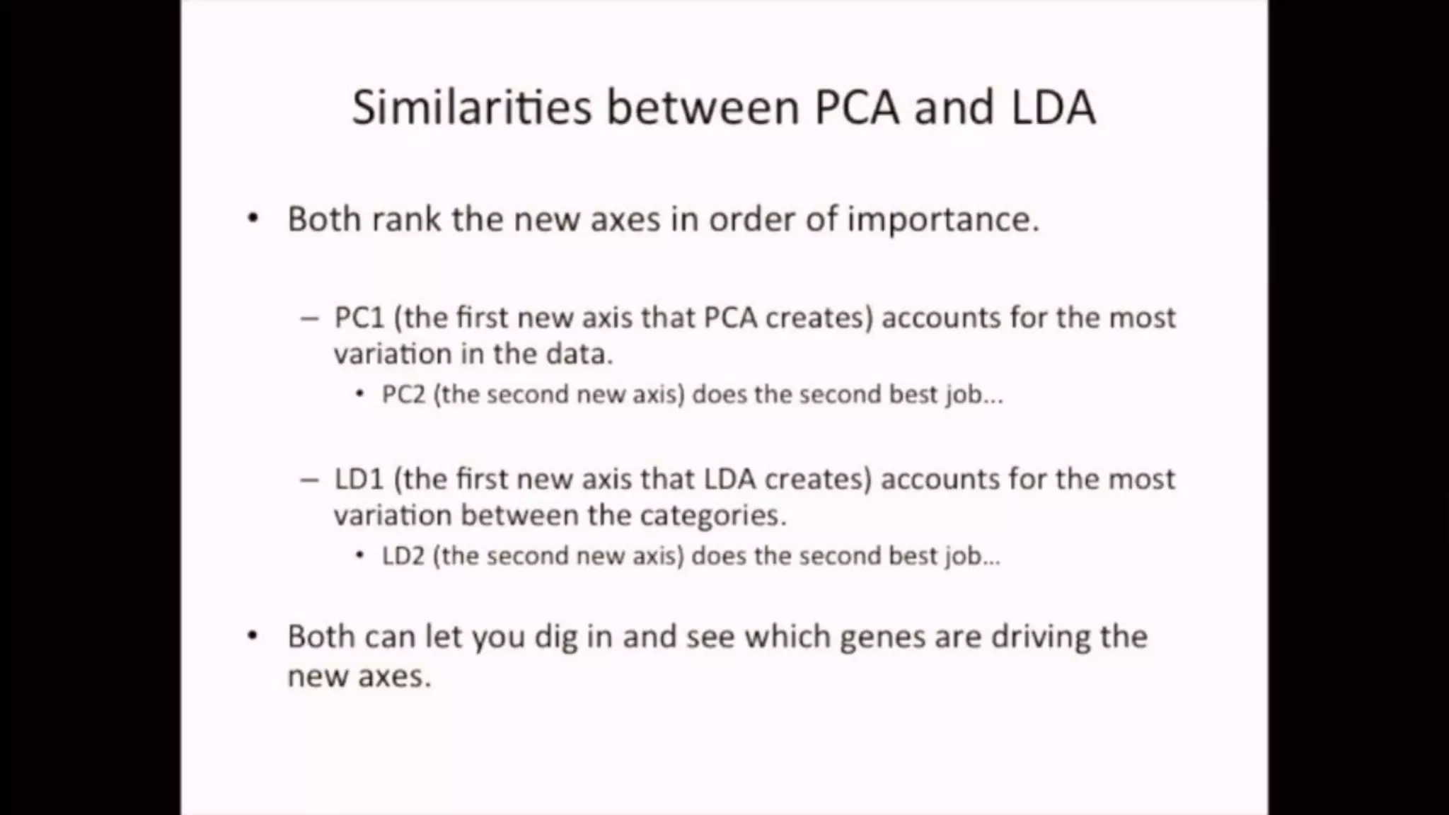
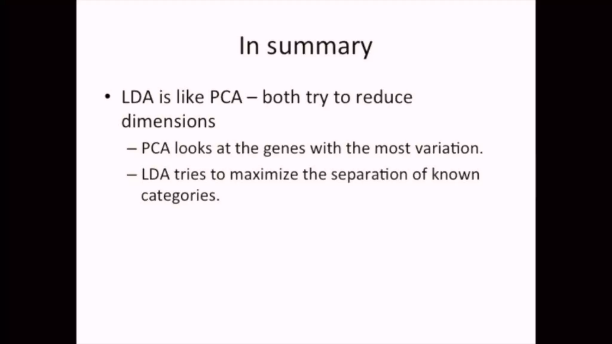
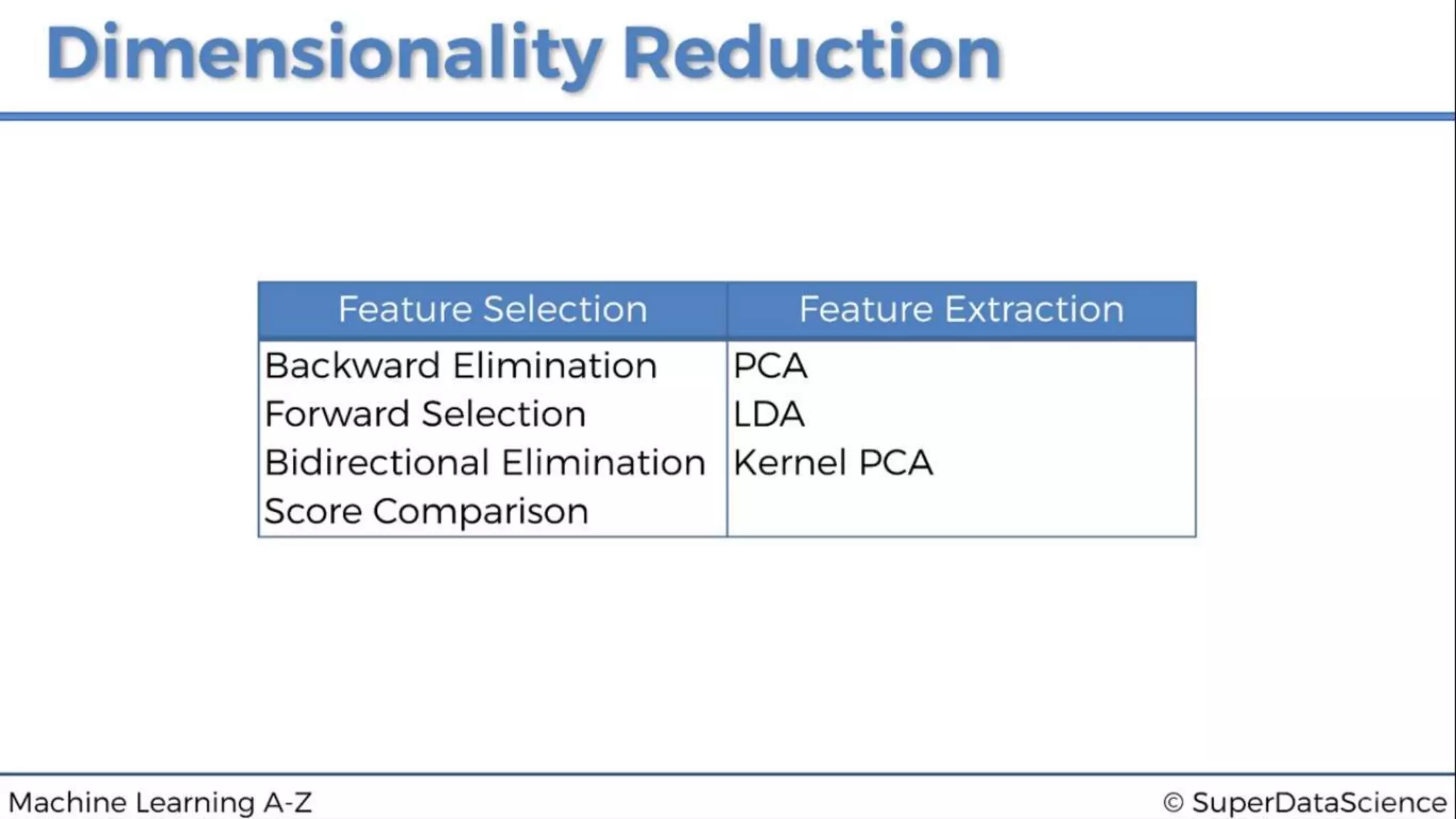
The document discusses Principal Component Analysis (PCA) and Linear Discriminant Analysis (LDA) as techniques for dimensionality reduction in machine learning. PCA is focused on maximizing variance retention while transforming correlated variables into principal components, whereas LDA aims to maximize class separability to improve classification performance. The text also includes Python code examples for implementing PCA and LDA, highlighting their applications in various domains such as finance and image processing.


![[DSC Europe 25] Boris Perkovic - Lost in performance.pptx](https://cdn.slidesharecdn.com/ss_thumbnails/uq5hrp7vsuahqkxzifux-1-251204082258-fd2ee09d-thumbnail.jpg?width=640&height=640&fit=bounds)


![[DSC Europe 25] Nikola Rajovic - Hardware Technologies Under the Hood: RISC-V...](https://cdn.slidesharecdn.com/ss_thumbnails/o2gptrmtoyqndgoshwgq-dsc2025-tenstorrent-rajovic-251205090438-814685f5-thumbnail.jpg?width=640&height=640&fit=bounds)

![[DSC Europe 25] Marija Vlajkovic & Andrea Radonjanin - Integration of AI tool...](https://cdn.slidesharecdn.com/ss_thumbnails/qf1jrglttoc3bm8s3aop-final-integration-of-ai-tools-251208151905-394f3a6a-thumbnail.jpg?width=640&height=640&fit=bounds)
![[DSC Europe 25] Goran Obradovic - The Rise of Sovereign AI: Building the Regi...](https://cdn.slidesharecdn.com/ss_thumbnails/7nw2xxixrxqdxvrb5wca-6-251205085714-ab09a2ac-thumbnail.jpg?width=640&height=640&fit=bounds)
![[DSC Europe 25] Dragan Vucic - Building the Learning Organization - How AI Tr...](https://cdn.slidesharecdn.com/ss_thumbnails/8brigo2sbu6qur6gxrra-7-251205085715-6ae07d24-thumbnail.jpg?width=640&height=640&fit=bounds)

![[DSC Europe 25] Dusan Jovicic - AI Story: From on-prem to cloud and back agai...](https://cdn.slidesharecdn.com/ss_thumbnails/8kp49m6uq22ifnbwhfnk-2-251205085715-964d11a6-thumbnail.jpg?width=640&height=640&fit=bounds)


