In this Scilab tutorial, we introduce readers to the Control System Toolbox that is available in Scilab/Xcos and known as CACSD. This first tutorial is dedicated to "Linear Time Invariant" (LTI) systems and their representations in Scilab.

1. www.openeering.com
powered by
INTRODUCTION TO CONTROL SYSTEMS IN SCILAB
In this Scilab tutorial, we introduce readers to the Control System Toolbox that is
available in Scilab/Xcos and known as CACSD. This first tutorial is dedicated to
"Linear Time Invariant" (LTI) systems and their representations in Scilab.
Level
This work is licensed under a Creative Commons Attribution-NonCommercial-NoDerivs 3.0 Unported License.

2. Control Systems in Scilab www.openeering.com page 2/17
Step 1: LTI systems
Linear Time Invariant (LTI) systems are a particular class of systems
characterized by the following features:
Linearity: which means that there is a linear relation between the
input and the output of the system. For example, if we scale and
sum all the input (linear combination) then the output are scaled
and summed in the same manner. More formally, denoting with
a generic input and with a generic output we have:
Time invariance: which mean that the system is invariant for
time translations. Hence, the output produced by the input
is identical to the output produced by the input
which is shifted by the quantity .
Thanks to these properties, in the time domain, we have that any LTI
system can be characterized entirely by a single function which is the
response to the system’s impulse. The system’s output is the
convolution of the input with the system's impulse response.
In the frequency domain, the system is characterized by the transfer
function which is the Laplace transform of the system’s impulse
response.
The same results are true for discrete time linear shift-invariant
systems which signals are discrete-time samples.

3. Control Systems in Scilab www.openeering.com page 3/17
Step 2: LTI representations
LTI systems can be classified into the following two major groups:
SISO: Single Input Single Output;
MIMO: Multiple Input Multiple Output.
LTI systems have several representation forms:
Set of differential equations in the state space representation;
Transfer function representation;
Zero-pole representation.
A typical representation of a system with its input and output ports and
its internal state
Step 3: RLC example
This RLC example is used to compare all the LTI representations. The
example refers to a RLC low passive filter, where the input is
represented by the voltage drop "V_in" while the output "V_out" is
voltage across the resistor.
In our examples we choose:
Input signal: ;
Resistor: ;
Inductor: ;
Capacitor: .
(Example scheme)

4. Control Systems in Scilab www.openeering.com page 4/17
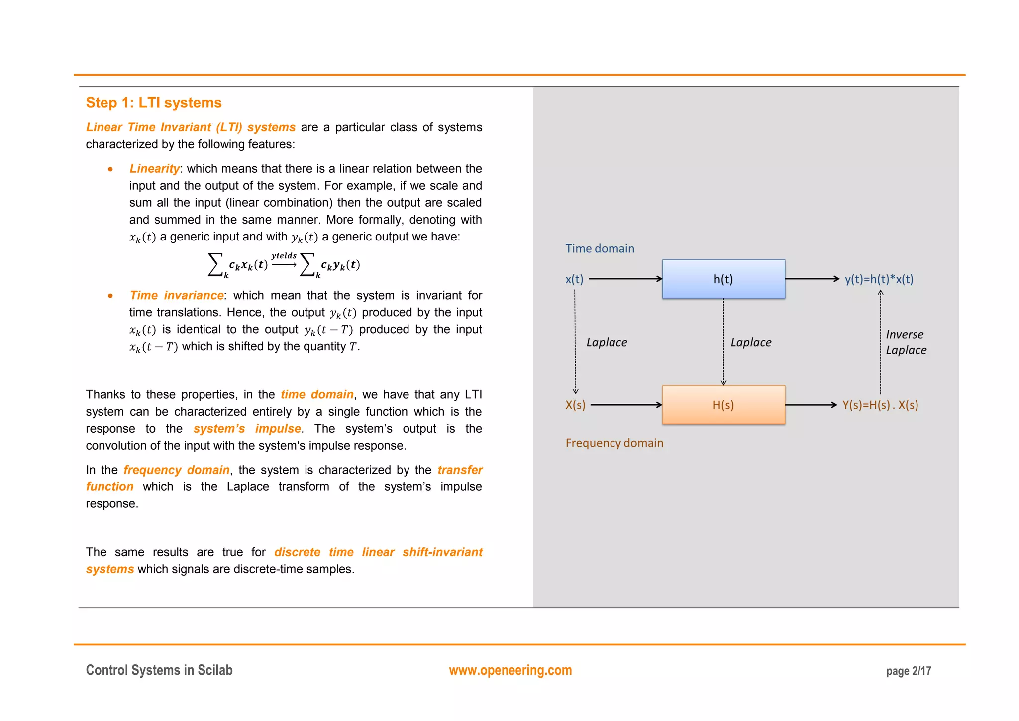
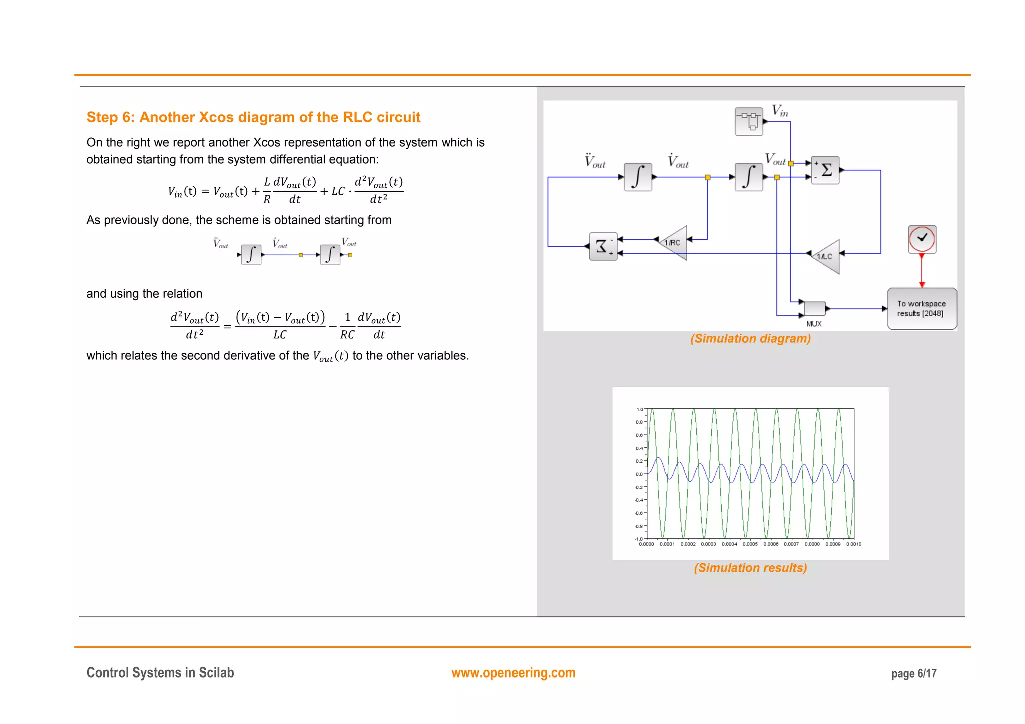
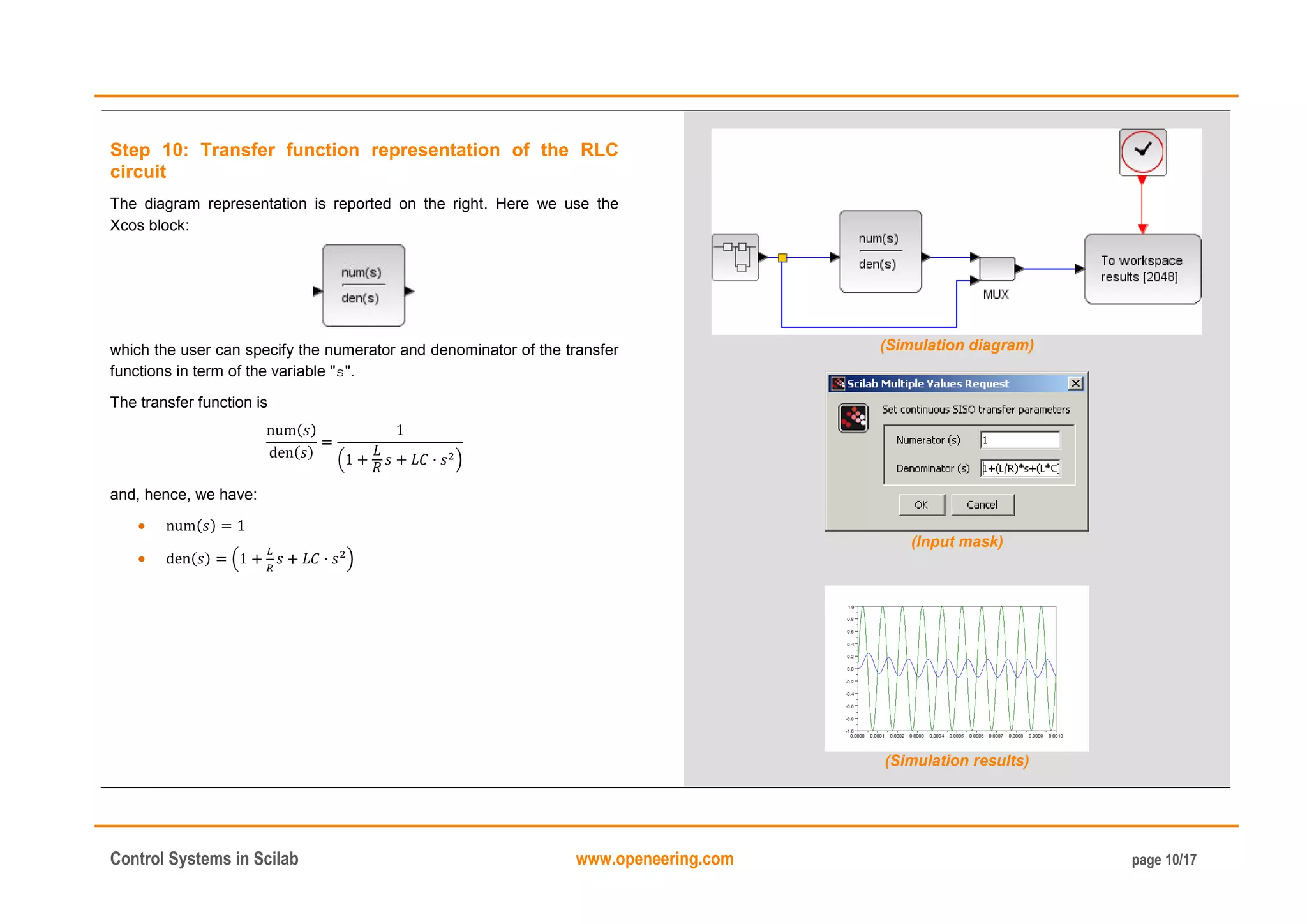
Step 4: Analytical solution of the RLC example
The relation between the input and the output of the system is:
On the right we report a plot of the solution for the following values of the
constants:
[V];
[Hz];
[Ohm];
[H];
[F];
with initial conditions: .
// Problem data
A = 1.0; f = 1e+4;
R = 10; // Resistor [Ohm]
L = 1e-3; // Inductor [H]
C = 1e-6; // Capacitor [F]
// Problem function
function zdot=RLCsystem(t, y)
z1 = y(1); z2 = y(2);
// Compute input
Vin = A*sin(2*%pi*f*t);
zdot(1) = z2; zdot(2) = (Vin - z1 - L*z2/R) /(L*C);
endfunction
// Simulation time [1 ms]
t = linspace(0,1e-3,1001);
// Initial conditions and solving the ode system
y0 = [0;0]; t0 = t(1);
y = ode(y0,t0,t,RLCsystem);
// Plotting results
Vin = A*sin(2*%pi*f*t)';
scf(1); clf(1); plot(t,[Vin,y(1,:)']); legend(["Vin";"Vout"]);
(Numerical solution code)
(Simulation results)

5. Control Systems in Scilab www.openeering.com page 5/17
Step 5: Xcos diagram of the RLC circuit
There can be many Xcos block formulation for the RLC circuit but the one
which allows fast and accurate results is the one that uses only
integration blocks instead of derivate blocks.
The idea is to start assembling the differential part of the diagram as:
and
and then to complete the scheme taking into consideration the relations
(Kirchhoff’s laws) and with .
At the end, we add the model for as follows:
The simulation results are stored in the Scilab mlist variable "results"
and plotted using the command
// Plotting data
plot(results.time,results.values)
(Simulation diagram)
(Simulation results)

6. Control Systems in Scilab www.openeering.com page 6/17
Step 6: Another Xcos diagram of the RLC circuit
On the right we report another Xcos representation of the system which is
obtained starting from the system differential equation:
As previously done, the scheme is obtained starting from
and using the relation
which relates the second derivative of the to the other variables.
(Simulation diagram)
(Simulation results)

7. Control Systems in Scilab www.openeering.com page 7/17
Step 7: State space representation
The state space representation of any LTI system can be stated as
follows:
where is the state vector (a collection of all internal variables that are
used to describe the dynamic of the system) of dimension , is the
output vector of dimension associated to observation and is the input
vector of dimension .
Here, the first equation represents the state updating equations while the
second one relates the system output to the state variables.
In many engineering problem the matrix is the null matrix, and hence
the output equation reduces to , which is a weight combination of
the state variables.
A space-state representation in term of block is reported on the right.
Note that the representation requires the choice of the state variable. This
choice is not trivial since there are many possibilities. The number of state
variables is generally equal to the order of the system’s differential
equations. In electrical circuit, a typical choice consists of picking all
variables associated to differential elements (capacitor and inductor).
State space representation
Block diagram representation of the state space equations

8. Control Systems in Scilab www.openeering.com page 8/17
Step 8: State space representation of the RLC circuit
In order to write the space state representation of the RLC circuit we
perform the following steps:
Choose the modeling variable: Here we use ,
and ;
Write the state update equation in the form ;
For the current in the inductor we have:
For the voltage across the capacitor we have:
Write the observer equation in the form .
The output voltage is equal to the voltage of the capacitor
. Hence the equation can be written as
The diagram representation is reported on the right using the Xcos block:
which can directly manage the matrices "A", "B", "C" and "D".
(Simulation diagram)
(Input mask)
(Simulation results)

9. Control Systems in Scilab www.openeering.com page 9/17
Step 9: Transfer function representation
In a LTI SISO system, a transfer function is a mathematical relation
between the input and the output in the Laplace domain considering its
initial conditions and equilibrium point to be zero.
For example, starting from the differential equation of the RLC example,
the transfer function is obtained as follows:
that is:
In the case of MIMO systems we don’t have a single polynomial transfer
function but a matrix of transfer functions where each entry is the transfer
function relationship between each individual input and each individual
output.
Examples of Laplace transformations:
Time domain Laplace domain

10. Control Systems in Scilab www.openeering.com page 10/17
Step 10: Transfer function representation of the RLC
circuit
The diagram representation is reported on the right. Here we use the
Xcos block:
which the user can specify the numerator and denominator of the transfer
functions in term of the variable "s".
The transfer function is
and, hence, we have:
(Simulation diagram)
(Input mask)
(Simulation results)

11. Control Systems in Scilab www.openeering.com page 11/17
Step 11: Zero-pole representation and example
Another possible representation is obtained by the use of the partial
fraction decomposition reducing the transfer function
into a function of the form:
where is the gain constant and and are, respectively, the zeros of
the numerator and poles of the denominator of the transfer function.
This representation has the advantage to explicit the zeros and poles of
the transfer function and so the performance of the dynamic system.
If we want to specify the transfer function in term of this representation in
Xcos, we can do that using the block
and specifying the numerator and denominator.
In our case, we have
with
(Simulation diagram)
(Input mask)
(Simulation results)

12. Control Systems in Scilab www.openeering.com page 12/17
Step 12: Converting between representations
In the following steps we will see how to change representation in Scilab
in an easy way. Before that, it is necessary to review some notes about
polynomial representation in Scilab.
A polynomial of degree is a function of the form:
Note that in Scilab the order of polynomial coefficient is reversed from that
of MATLAB
®
or Octave
®
.
The main Scilab commands for managing polynomials are:
%s: A Scilab variable used to define polynomials;
poly: to create a polynomial starting from its roots or its
coefficients;
coeff: to extract the coefficient of the polynomial;
horner: to evaluate a polynomial;
derivat: to compute the derivate of a polynomial;
roots: to compute the zeros of the polynomial;
+, -, *: standard polynomial operations;
pdiv: polynomial division;
/: generate a rational polynomial i.e. the division between two
polynomials;
inv or invr: inversion of (rational) matrix.
// Create a polynomial by its roots
p = poly([1 -2],'s')
// Create a polynomial by its coefficient
p = poly([-2 1 1],'s','c')
// Create a polynomial by its coefficient
// Octave/MATLAB(R) style
pcoeff = [1 1 -2];
p = poly(pcoeff($:-1:1),'s','c')
pcoeffs = coeff(p)
// Create a polynomial using the %s variable
s = %s;
p = - 2 + s + s^2
// Another way to create the polynomial
p = (s-1)*(s+2)
// Evaluate a polynomial
res = horner(p,1.0)
// Some operation on polynomial, sum, product and find zeros
q = p+2
r = p*q
rzer = roots(r)
// Symbolic substitution and check
pp = horner(q,p)
res = pp -p-p^2
typeof(res)
// Standard polynomial division
[Q,R] = pdiv(p,q)
// Rational polynomial
prat = p/q
typeof(prat)
prat.num
prat.den
// matrix polynomial and its inversion
r = [1 , 1/s; 0 1]
rinv = inv(r)

13. Control Systems in Scilab www.openeering.com page 13/17
Step 13: Converting between representations
The state-space representation of our example is:
while the transfer function is
In Scilab it is possible to move from the state-space representation to the
transfer function using the command ss2tf. The vice versa is possible
using the command tf2ss.
In the reported code (right), we use the "tf2ss" function to go back to the
previous state but we do not find the original state-space representation.
This is due to the fact that the state-space representation is not unique
and depends on the adopted change of variables.
The Scilab command ss2ss transforms the system through the use of a
change matrix , while the command canon generates a transformation
of the system such that the matrix "A" is on the Jordan form.
The zeros and the poles of the transfer function can be display using the
command trfmod.
// RLC low passive filter data
mR = 10; // Resistor [Ohm]
mL = 1e-3; // Inductor [H]
mC = 1e-6; // Capacitor [F]
mRC = mR*mC;
mf = 1e+4;
// Define system matrix
A = [0 -1/mL; 1/mC -1/mRC];
B = [1/mL; 0];
C = [0 1];
D = [0];
// State space
sl = syslin('c',A,B,C,D)
h = ss2tf(sl)
sl1 = tf2ss(h)
// Transformation
T = [1 0; 1 1];
sl2 = ss2ss(sl,T)
// Canonical form
[Ac,Bc,U,ind]=canon(A,B)
// zero-poles
[hm]=trfmod(h)
(Output of the command trfmod)

14. Control Systems in Scilab www.openeering.com page 14/17
Step 14: Time response
For a LTI system the output can be computed using the formula:
In Scilab this can be done using the command csim for continuous
system while the command dsimul can be used for discrete systems.
The conversion between continuous and discrete system is done using
the command dscr specifying the discretization time step.
On the right we report some examples: the transfer function is relative to
the RLC example.
// the step response (continuous system)
t = linspace(0,1e-3,101);
y = csim('step',t,sl);
scf(1); clf(1);
plot(t,y);
// the step response (discrete system)
t = linspace(0,1e-3,101);
u = ones(1,length(t));
dt = t(2)-t(1);
y = dsimul(dscr(h,dt),u);
scf(2); clf(2);
plot(t,y);
// the user define response
t = linspace(0,1e-3,1001);
u = sin(2*%pi*mf*t);
y = csim(u,t,sl);
scf(3); clf(3);
plot(t,[y',u']);

15. Control Systems in Scilab www.openeering.com page 15/17
Step 15: Frequency domain response
The Frequency Response is the relation between input and output in the
complex domain. This is obtained from the transfer function, by
replacing with .
The two main charts are:
Bode diagram: In Scilab this can be done using the command
bode;
And Nyquist diagram: In Scilab this can be done using the
command nyquist.
// bode
scf(4); clf(4);
bode(h,1e+1,1e+6);
// Nyquist
scf(5); clf(5);
nyquist(sl,1e+1,1e+6);
(Bode diagram)
(Nyquist diagram)

16. Control Systems in Scilab www.openeering.com page 16/17
Step 16: Exercise
Study in term of time and frequency responses of the following RC band-
pass filter:
Use the following values for the simulations:
[Ohm];
[F];
[Ohm];
[F].
Hints: The transfer function is:
The transfer function can be defined using the command syslin.
(step response)
(Bode diagram)
(Nyquist diagram)

17. Control Systems in Scilab www.openeering.com page 17/17
Step 17: Concluding remarks and References
In this tutorial we have presented some modeling approaches in
Scilab/Xcos using the Control System Toolbox available in Scilab known
as CACSD.
1. Scilab Web Page: Available: www.scilab.org.
2. Openeering: www.openeering.com.
Step 18: Software content
To report bugs or suggest improvements please contact the Openeering
team.
www.openeering.com.
Thanks for the bug report: Konrad Kmieciak.
Thank you for your attention,
Manolo Venturin
--------------
Main directory
--------------
ex1.sce : Exercise 1
numsol.sce : Numerical solution of RLC example
poly_example.sce : Polynomial in Scilab
RLC_Xcos.xcos : RLC in standard Xcos
RLC_Xcos_ABCD.xcos : RLC in ABCD formulation
RLC_Xcos_eq.xcos : Another formulation of RLC in Xcos
RLC_Xcos_tf.xcos : RLC in transfer function form.
RLC_Xcos_zp.xcos : RLC in zeros-poles form.
system_analysis.sce : RLC example system analysis
license.txt : The license file