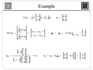
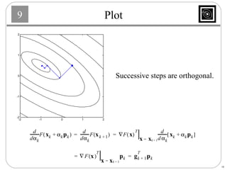
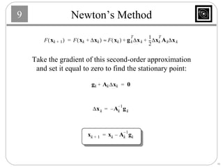
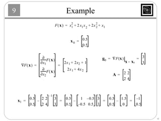
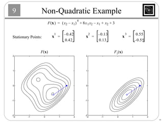
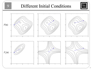
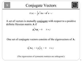
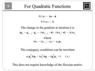
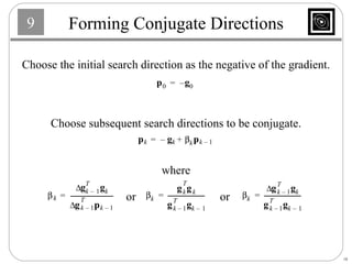
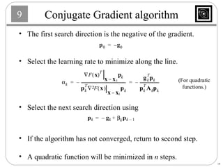
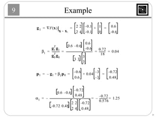
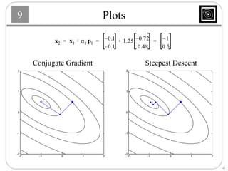
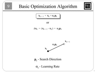
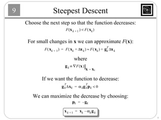
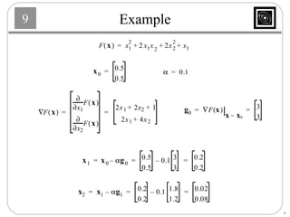
This document discusses several basic optimization algorithms: 1) Steepest descent chooses the search direction to maximize decrease in the function at each step. 2) Newton's method approximates the function as a quadratic and finds the stationary point by setting the gradient of this approximation to zero. 3) Conjugate gradient methods choose subsequent search directions to be conjugate to improve convergence for non-quadratic functions. The directions are updated to be conjugate to previous directions.

1. Performance Optimization

2. Basic Optimization Algorithm p k - Search Direction  k - Learning Rate or

3. Steepest Descent Choose the next step so that the function decreases: For small changes in x we can approximate F ( x ): where If we want the function to decrease: We can maximize the decrease by choosing:

4. Example

5. Plot

6. Stable Learning Rates (Quadratic) Stability is determined by the eigenvalues of this matrix. Eigenvalues of [ I -  A ]. Stability Requirement: (  i - eigenvalue of A )

7. Example

8. Minimizing Along a Line Choose  k to minimize where

9. Example

10. Plot Successive steps are orthogonal. F x    T x x k 1 + = p k g k 1 + T p k = =

11. Newton’s Method Take the gradient of this second-order approximation and set it equal to zero to find the stationary point:

12. Example

13. Plot

14. Non-Quadratic Example Stationary Points: F ( x ) F 2 ( x )

15. Different Initial Conditions F ( x ) F 2 ( x )

16. Conjugate Vectors A set of vectors is mutually conjugate with respect to a positive definite Hessian matrix A if One set of conjugate vectors consists of the eigenvectors of A . (The eigenvectors of symmetric matrices are orthogonal.)

17. For Quadratic Functions The change in the gradient at iteration k is where The conjugacy conditions can be rewritten This does not require knowledge of the Hessian matrix.

18. Forming Conjugate Directions Choose the initial search direction as the negative of the gradient. Choose subsequent search directions to be conjugate. where or or

19. Conjugate Gradient algorithm The first search direction is the negative of the gradient. Select the learning rate to minimize along the line. Select the next search direction using If the algorithm has not converged, return to second step. A quadratic function will be minimized in n steps. (For quadratic functions.)

20. Example

21. Example

22. Plots Conjugate Gradient Steepest Descent