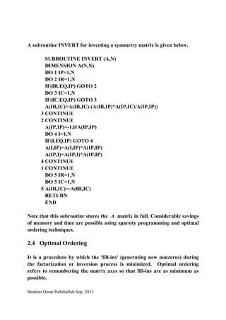
This document discusses two triangular factorization techniques - LU factorization and Cholesky-Coleman matrix inversion - that can be used to solve simultaneous linear equations in matrix form. LU factorization involves factorizing a matrix A into lower and upper triangular matrices L and U. Cholesky-Coleman matrix inversion allows in-situ inversion of a nonsingular square matrix. Optimal ordering techniques are also introduced, which aim to minimize "fill-ins" or new nonzeros generated during factorization or inversion to maintain sparsity. Examples are provided to demonstrate applying LU factorization and Cholesky-Coleman inversion to solve systems of equations.
![Ibrahim Omar Habiballah Sep. 2013
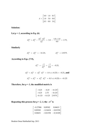
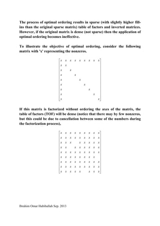
If the first pivot is moved to the last axis, i.e.,
⎥
⎥
⎥
⎥
⎥
⎥
⎥
⎥
⎥
⎥
⎥
⎥
⎦
⎤
⎢
⎢
⎢
⎢
⎢
⎢
⎢
⎢
⎢
⎢
⎢
⎢
⎣
⎡
xxxxxxxxx
xx
xx
xx
xx
xx
xx
xx
xx
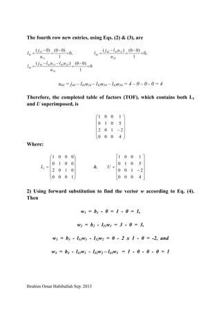
then the table of factors (TOF) will be sparse, and for this particular
matrix structure, the TOF will have same sparse structure but with
different nonzero (fill-ins) values.
References:
[1] G.T. Heydt, "Computer Analysis Methods for Power System",
Macmillan, New York, 1986.](https://image.slidesharecdn.com/04programming-2-190410143727/85/04-programming-2-10-320.jpg)