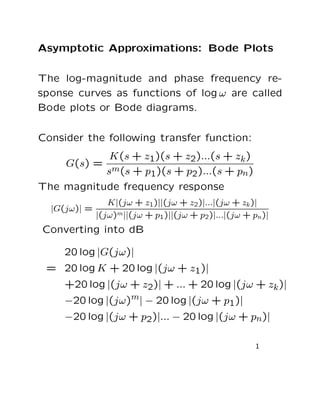
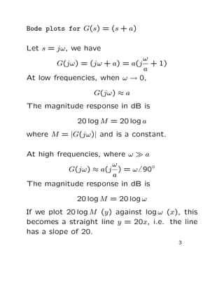
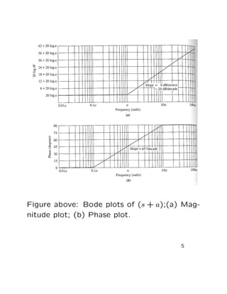
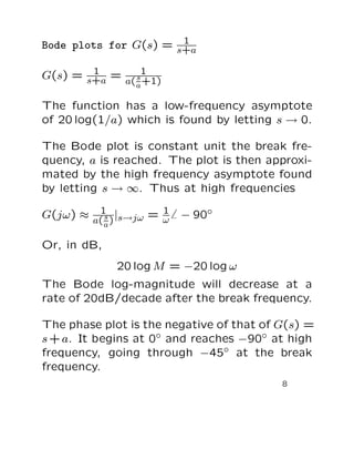
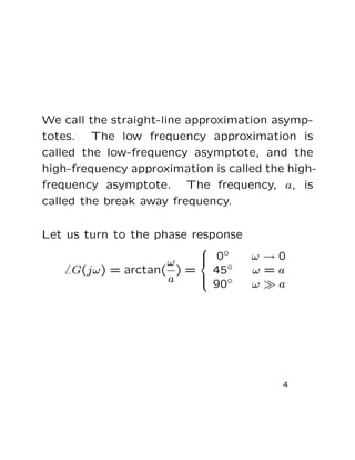
Bode plots show the magnitude and phase response of a system as functions of frequency. They can be approximated as a sequence of straight lines called asymptotes. For a transfer function G(s) = (s + a), the Bode plot has: 1) A low-frequency asymptote of 20 log(a) where the magnitude is constant. 2) At the break frequency a, the phase reaches -45 degrees. 3) A high-frequency asymptote where the magnitude decreases at -20dB/decade and the phase reaches -90 degrees. Normalizing the transfer function allows the break frequency to appear at 1 rad/sec on the plot. Bode plots

1. Asymptotic Approximations: Bode Plots
The log-magnitude and phase frequency re-
sponse curves as functions of log ω are called
Bode plots or Bode diagrams.
Consider the following transfer function:
K(s + z1)(s + z2)...(s + zk )
G(s) = m
s (s + p1)(s + p2)...(s + pn)
The magnitude frequency response
K|(jω + z1)||(jω + z2 )|...|(jω + zk )|
|G(jω)| =
|(jω)m||(jω + p1 )||(jω + p2)|...|(jω + pn)|
Converting into dB
20 log |G(jω)|
= 20 log K + 20 log |(jω + z1)|
+20 log |(jω + z2)| + ... + 20 log |(jω + zk )|
−20 log |(jω)m| − 20 log |(jω + p1)|
−20 log |(jω + p2)|... − 20 log |(jω + pn)|
1

2. Thus if we know the magnitude response of
each term, we can find the total magnitude
response by adding zero terms’ magnitude re-
sponses and subtracting pole terms’ magnitude
responses.
Similarly if we know the phase response of each
term, we can find the total phase response by
adding zero terms’ phase responses and sub-
tracting pole terms’ phase responses.
Sketching Bode plots can be simplified because
they can be approximated as a sequence of
straight lines.
2

3. Bode plots for G(s) = (s + a)
Let s = jω, we have
ω
G(jω) = (jω + a) = a(j + 1)
a
At low frequencies, when ω → 0,
G(jω) ≈ a
The magnitude response in dB is
20 log M = 20 log a
where M = |G(jω)| and is a constant.
At high frequencies, where ω ≫ a
ω
G(jω) ≈ a(j ) = ω 90◦
a
The magnitude response in dB is
20 log M = 20 log ω
If we plot 20 log M (y) against log ω (x), this
becomes a straight line y = 20x, i.e. the line
has a slope of 20.
3

4. We call the straight-line approximation asymp-
totes. The low frequency approximation is
called the low-frequency asymptote, and the
high-frequency approximation is called the high-
frequency asymptote. The frequency, a, is
called the break away frequency.
Let us turn to the phase response
 0◦

ω→0
ω 
G(jω) = arctan( ) = 45◦ ω=a
a  90◦

ω≫a
4

5. Figure above: Bode plots of (s + a);(a) Mag-
nitude plot; (b) Phase plot.
5

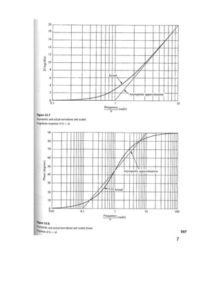
6. It is often convenient to normalize the magni-
tude and scale the frequency so that the log-
magnitude plot will be 0 dB at a break fre-
quency of unity.
To normalize (s+a) we factor out the quantity
a and form a[(s/a) + 1]. By defining a new fre-
quency variable s1 = s/a, the normalized scaled
function is s1 + 1. To obtain the original fre-
quency response, the magnitude and frequency
are multiplied by the quantity a.
The actual magnitude curve is never greater
than 3.01 dB from the asymptote. The maxi-
mum difference occurs at break away frequency.
The maximum difference for the phase curve is
5.71◦, which occurs at the decades above and
below the break frequency.
6

7. 7

8. 1
Bode plots for G(s) = s+a
G(s) = s+a = a( s1
1
a +1)
The function has a low-frequency asymptote
of 20 log(1/a) which is found by letting s → 0.
The Bode plot is constant unit the break fre-
quency, a is reached. The plot is then approxi-
mated by the high frequency asymptote found
by letting s → ∞. Thus at high frequencies
1 1
G(jω) ≈ a( s ) |s→jω = ω − 90◦
a
Or, in dB,
20 log M = −20 log ω
The Bode log-magnitude will decrease at a
rate of 20dB/decade after the break frequency.
The phase plot is the negative of that of G(s) =
s + a. It begins at 0◦ and reaches −90◦ at high
frequency, going through −45◦ at the break
frequency.
8

9. Bode plots for G(s) = s
G(s) = s has only a high-frequency asymp-
tote. The magnitude plot is straight line with
20dB/decade slope passing 0 dB when ω = 1.
The phase plot has a constant 90◦.
Bode plots for G(s) = 1
s
The magnitude plot for G(s) = 1 is a straight
s
line with -20dB/decade slope passing 0 dB
when ω = 1.
The phase plot has a constant −90◦.
9

10. Figure above; Normalized and scaled Bode plots
for (a) G(s) = s; (b) G(s) = 1 ; (c) G(s) =
s
1 .
s + a; and (d) G(s) = s+a
10