plotting bode plot.

1. 1.6. ILLUSTRATIVE PROBLEMS AND SOLUTIONS
This section provides a set of illustrative problems and their solutions to supplement the
material presented in Chapter 1.
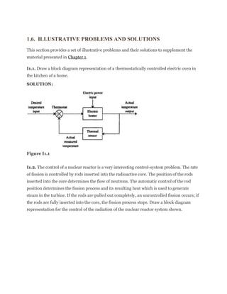
I1.1. Draw a block diagram representation of a thermostatically controlled electric oven in
the kitchen of a home.
SOLUTION:
Figure I1.1
I1.2. The control of a nuclear reactor is a very interesting control-system problem. The rate
of fission is controlled by rods inserted into the radioactive core. The position of the rods
inserted into the core determines the flow of neutrons. The automatic control of the rod
position determines the fission process and its resulting heat which is used to generate
steam in the turbine. If the rods are pulled out completely, an uncontrolled fission occurs; if
the rods are fully inserted into the core, the fission process stops. Draw a block diagram
representation for the control of the radiation of the nuclear reactor system shown.

2. Figure I1.2i
SOLUTION:
Figure I1.2ii
I1.3. The automatic depth control of a submarine is an interesting control system problem.
Suppose the captain of the submarine wants the submarine to “hover” at a desired depth,
and sets the desired depth as a voltage from a calibrated potentiometer. The actual depth is
measured by a pressure transducer which produces a voltage proportional to depth. The
following figure illustrates the problem, where the actual depth of the submarine is denoted
as C. Any differences are amplified which then drives a motor that rotates the stern plane
actuator angle θ in order that the stern plane rotation reduces the depth error of the
submarine to zero. Draw the block diagram representation of the automatic depth control
system of the submarine.

3. Figure I1.3i
SOLUTION:
Figure I1.3ii
I1.4. An elevator-position control system used in an apartment building is a very interesting
control-system problem. Draw the block diagram representation of an elevator control
system in a three-floor building which obtains the desired floor reference position as a
voltage from the elevator passenger pressing a button on the elevator, and compares this
voltage with a voltage from a position sensor that represents the actual floor position the
elevator is at. The difference is an error voltage which is amplified and connected to an
electric motor that positions the elevator car to the desired floor selected.
SOLUTION:

4. Figure I1.4
BODE DIAGRAMS USING MATLAB [7]
In the previous section, several Bode diagrams were illustrated whose amplitude plots were
obtained from hand-drawn straight-line asymptotic slopes and whose phase characteristics
were calculated from the appropriate trigonometric fucntions. Additionally, several Bode
diagrams were also illustrated which were obtained using MATLAB. In this section, the
reader will be shown how to obtain the Bode diagrams very easily and accurately using
MATLAB.
Let us practice creating Bode diagrams using MATLAB. There are many examples to
practice with for creating Bode diagrams on the Modern Control System Theory and
Design (MCSTD) Toolbox. Two functions exist that assist in Bode diagrams:
1. “bode” returns/plots the Bode response of a system.
2. “margins” is described in the MCSTD toolbox. This, in my opinion, has an advantage
over the professional version of the Control System toolbox’s “margin” routine.
Margins analytically calculates, with analytic precision, the gain and phase margins
and their associated frequencies (versus interpolating a single value from a plot).
When trying to find the proper syntax to call the “bode” utility, either use the help feature or
look in the reference manual. I personally prefer the help feature, unless I need an example.
Valid syntax for the “bode” utility, for transfer functions, is:
1. [mag,phase,w] = bode(num,den)
2. [mag,phase,w] = bode(num,den,w)

5. 3. [mag,phase] = bode(num,den,w)
4. bode(num,den,w)
5. bode(num,den)
The left-hand arguments (mag, phase and w) are optional for this function, as described on
the second page of the Bode function in The Student Edition book. The result, which can be
manually typed, is listed below so that you may try the Bode example in the book:
a = [0, 1; −1. −0.4];
b = [0; 1];
c = [1, 0];
d = 0;
A major short-coming of the Bode diagram is that the margins (gain and phase) are not put
onto the plot when it generates the plots. The effect of this is compounded when you want to
put them onto the plot, and you discover that you can only modify the phase plot with
reasonable ease. Adding to the magnitude plot is almost impossible (prior to MATLAB
version 4.0). This is why they have the left-hand arguments, so that you can generate the
Bode plots yourself with whatever customization on the plot that you desire. This is what is
accomplished in the MCSTD Toolbox when Bode diagrams are obtained in the DEMO,
figures, or problems directory.
A. Drawing the Bode Diagram if the System is Defined by a Transfer Function
To illustrate the use of MATLAB for obtaining the Bode diagram, let us consider the
following example. The open-loop transfer function of a control system is given by the
following:
In order to ease its transformation to MATLAB notation, we multiply all terms in the
numerator and denominator as follows:

6. Therefore, the row matrices for the numerator and denominator are as follows:
num = [0 0 0 1 44 160]
den = [1 1100 180,000 0 0 0].
The resulting MATLAB program will first be provided by the listing in Table 6.8, and new
commands will then be explained. The resulting Bode diagram is shown in Figure 6.35.
MATLAB and the MCSTD Toolbox automatically select the frequency range used in Figure
6.35 when using the MATLAB program in Table 6.8. If the control-system engineer wants to
select a different frequency range, such as from 0.01 to 10,000 rad/sec instead of from 0.1 to
10,000 rad/sec, then we have to use the “log-space” command which is defined as follows:
Table 6.8. MATLAB Program for Obtaining Bode Diagram of System Defined
in Eq. (6.106)
num = [0 0 0 1 44 160];
den = [1 1100 180000 0 0 0];
w = logspace(−2, 4);
[mag,ph] = bode(num,den);
grid
title(‘Bode Diagram of
G(s)H(s) = (s + 4)(s + 40)/s^3(s + 200)(s + 900)’)

7. Figure 6.35 Bode diagram for control system whose transfer function is defined by Eq.
(6.105).
w = logspace(−2,
4):
Generates 50 points equally spaced between ω = 10−2
and
104
rad/sec
In addition, we now have to use the MATLAB command “bode(num,den,w)” which is
defined as follows:
bode(num,den,w): Generates the Bode diagram from the user-supplied num,
den, and the frequency vector wwhich specifies the
frequencies at which the Bode diagram will be calculated.
Using the MATLAB commands “logspace” and “bode(num,den,w)”, in the MATLAB
Program in Table 6.8, is modified as shown in the MATLAB Program in Table 6.9.
Table 6.9. MATLAB Program for Obtaining Bode Diagram of System Defined
in Eq. (6.106) with the Logspace Command

8. num = [0 0 0 1 44 160];
den = [1 1100 180000 0 0 0];
w = logspace(−2,4);
[mag,ph] = bode(num,den,w);
grid
title (‘Bode Diagram of
G(s)H(s) = (s + 4)(s + 40)/s3
(s + 200)(s + 900)’)
Figure 6.36 Bode diagram of G(s)H(s) = with the logspace command
added.
The resulting Bode diagram is shown in Figure 6.36. Observe that the frequency range of
this Bode diagram is 0.01 to 10,000 rad/sec, compared to 0.1 to 10,000 rad/sec in Figure
6.35.
The MCSTD Toolbox command margins provide the following:

9. ‡ gain margin (gm)
‡ phase margin (pm)
‡ frequency (rad/sec) where the phase equals −180° (wcg: ωcg, gain crossover frequency)
‡ frequency (rad/sec) where the gain equals zero dB (wcp: ωcp, phase crossover frequency).
Therefore, adding the following MCSTD Toolbox command to the MATLAB Program
in Table 6.9,
[gm, pm, wcg, wcp] = margins(num,den)
will result in the Bode diagram of Figure 6.37 which contains everything previously shown
on Figure 6.36 plus the phase margin, the gain margin, the frequency where the gain equals
zero dB, and the frequencies where the phase is −180°. Observe from Figure 6.37 that this
control system has two gain margins and one phase margin.
Therefore, the MCSTD Toolbox enhances MATLAB. The MCSTD Toolbox DEMO M-file
elaborates further on the creation of the Bode diagram with several on-screen examples.
B. Drawing the Bode Diagram if the System is Defined in State-Space Form
The MATLAB command for this case is given by
bode(A,B,C,D).

10. Figure 6.37 Bode diagram of G(s)H(s) = with the logspace command
added.
As was demonstrated previously in this chapter (e.g., Section 6.6 on the Nyquist Diagram),
we must first obtain the state-space form and then use this new command.
To demonstrate this procedure, let us obtain the state-space form from the transfer function
given by Eq. (6.106) using the MATLAB command
[A,B,C,D] = tf2ss(num,den)
whose application has been demonstrated earlier in the section on the Nyquist diagram
(Section 6.6). The resulting MATLAB program for accomplishing this is shown in the
MATLAB program in Table 6.10.
Therefore, the resulting MATLAB program for obtaining the Bode diagram of this problem
from the state-space formulation is given by the MATLAB program in Table 6.11. The
resulting Bode diagram is identical to that shown in Figure 6.36.

11. Table 6.11. MATLAB Program for Determining the Bode Diagram from the
State-Space Form.
A = [−1100 − 180000 0 0 0; 1 0 0 0 0; 0 1 0 0 0;
0 0 1 0 0; 0 0 0 1 0]
B = [1; 0; 0; 0; 0]
C = [0 0 1 44 160];
D = [0];
w = logspace(−2,4);
[mag, ph] = bode(A,B,C,D,w)
grid
title(‘Bode Diagram of
G(s)H(s) = (s + 4)(s + 40)/s^3(s + 200)(s + 900)’)