This document discusses biosignal processing and covers the following key points in 3 sentences: It provides an overview of biosignal processing techniques including filtering to remove artifacts, event detection, and compression. It defines biosignals and gives examples like ECG and EMG. The document outlines topics like characterizing biosignals in the time and frequency domains, and techniques for time-frequency analysis like short-time Fourier transform and wavelet transform.

1. Smart Tech: Biosignals & Medical Electronics
Biosignal processing
Oresti Banos
May 19th, 2017
o.banoslegran@utwente.nl
@orestibanos
http://orestibanos.com/
19-Apr-18 1

2. Biosignal processing in the overall “biopicture”
19-Apr-18 2
Lectures 1, 2, 3
Lecture 4 (today)Lecture 5 (next week)
Biosignal acquisition
Biosignal processingBiodata analysis

3. Learning Objectives
At the end of this course you should be able to:
 Explain the concept of (bio)signal
and identify some of the most
common types of biosignals
 Describe the main characteristics of
biosignals in both time and
frequency domains
 Apply regular processing techniques
for the removal of common artifacts
in biosignals
 Utilise typical processing techniques
for the detection of relevant events
in biosignals
19-Apr-18 3

4. Outline
 Biosignal definition
 Time and frequency
characterisation of biosignals
 Biosignal processing
 Filtering for removal of artifacts
 Event detection
 Compression
19-Apr-18 4

5. Outline
 Biosignal definition
 Time and frequency
characterisation of biosignals
 Biosignal processing
 Filtering for removal of artifacts
 Event detection
 Compression
19-Apr-18 5

6. Biosignal: definition
 Signal: function that "conveys information about
the behavior or attributes of some phenomenon”
 Biosignal (also biomedical signal, bioelectrical
signal or physiological signal):
 “any biological quantity or magnitude exhibiting variation
in time or variation in space is potentially a signal that
provides information on the status of a biological system”
19-Apr-18 6
 In time (1D): e.g., electrocardiogram (ECG)
measures heart activity by detecting changes
associated with heart muscle contractions
 In space (2D): e.g., functional magnetic
resonance imaging (fMRI) measures brain
activity by detecting changes associated with
blood flow
 In time-space (3D): e.g., a medical ultrasound
measures surface or internal organs structural
movements by detecting changes in the
reflection of sound waves on the tissues

7. Biosignal: examples
19-Apr-18 7
Electroencephalogram
(EEG)
Electroneurogram
(ENG)
Electroretinogram
(ERG)
Electrooculogram
(EOG)
Electroogastrogram
(EGG)
Phonocardiogram (PCG),
Photopletismogram (PPG),
Vibromyogram (VMG),
Vibroarthrogram (VAG), …
and also Speech, Motion,
etc.!!

8. ECG
 Electrocardiogram (ECG or EKG):
 Electrical activity of the heart, measured through
electrodes on chest, arms, and legs
 An electrical impulse travels through the heart
determining its rhythm and rate, and causing the heart
muscle to contract and pump blood
 Typical ECG signals are between 0.1 to 2 mV and
appear with frequency of 0.6 – 50 Hz
19-Apr-18 8

9. ECG
https://www.youtube.com/watch?v=KWrzdJY4G9Q
19-Apr-18 9

10. EMG
 Electromiogram (EMG):
 Electrical activity of skeletal muscles (usually
proportional to the level of activity)
 Recorded through electrodes on the skin overlying the
muscle
 Typical EMG signals are between 100 – 300 µV and
appear with frequency of 6 – 30 Hz
 Videos:
 goo.gl/Qxegu5
19-Apr-18 10

11. Outline
 Biosignal definition
 Time and frequency
characterisation of biosignals
 Biosignal processing
 Filtering for removal of artifacts
 Event detection
 Compression
19-Apr-18 11

12. Biosignals: time-domain characterisation
 Signal domain
 Continuous-time  Signal as a function of time x(t)
 e.g., temperature measured seamlessly
 Discrete-time  Signal as a function of samples x(n)
 e.g., temperature measured every hour
 Digital  Discrete-time signal with values limited to
quantised levels ẋ(n)
 e.g., temperature measured every hour with a resolution of 1ºC
19-Apr-18 12
13:00 14:00 15:00 16:00 17:00 18:00
Time (h)
35
35.5
36
36.5
37
37.5
38
Temp(°C)
13:00 14:00 15:00 16:00 17:00 18:00
Time (h)
35
35.5
36
36.5
37
37.5
38
Temp(°C)
13:00 14:00 15:00 16:00 17:00 18:00
Time (h)
35
35.5
36
36.5
37
37.5
38
Temp(°C)𝑥(𝑡) 𝑥(𝑛) 𝑥(𝑛)

13. Biosignals: time-domain characterisation
 Sampling rate
 Frequency at which a continuous signal is sampled
 Shannon-Nyquist theorem: fsampling ≧ 2fmax,signal = 2BW
Temporal aliasing Spatial aliasing
19-Apr-18 13
0 0.5 1 1.5 2 2.5 3 3.5 4 4.5 5
-1
-0.5
0
0.5
1
1.5
2
0 0.5 1 1.5 2 2.5 3 3.5 4 4.5 5
-1
-0.5
0
0.5
1
1.5
2
0 0.5 1 1.5 2 2.5 3 3.5 4 4.5 5
-1
-0.5
0
0.5
1
1.5
2
0 0.5 1 1.5 2 2.5 3 3.5 4 4.5 5
-1
-0.5
0
0.5
1
1.5
2
Adequately sampled ECG
Aliased ECG Aliased MRI

14. Biosignals: time-domain characterisation
 Amplitude
 Describes the intensity of the biological phenomenon
(a.k.a, dependent variable, range, or ordinate)
 Not to be confused with range or peak-to-peak amplitude
 Duration
 Signals are considered to exist for all time (e.g., sin(wt))
 We normally take “just” some samples of the signal
(subpart or realisation of the actual signal)
19-Apr-18 14

15. Biosignals: time-domain characterisation
 Periodicity
 Periodic: the shape of the signal repeats with an interval
 Aperiodic: the shape of the signal never repeats
 Predictability
 Deterministic: predictable for the time span of interest
 Random: signal values cannot be precisely anticipated
 Stationary: (nearly) constant statistics or frequency spectra over time
 Non-stationary: varying statistics or frequency spectra over time
19-Apr-18 15
MATLAB: rand
 Some biosignals are considered
quasi-periodic (e.g., ECG, BP)
 Most biosignals are aperiodic
and non-stationary (e.g., EEG,
EMG)
EEG
BP
ECG

16. Biosignals: time-domain characterisation
 Time-domain parameters (A,B,C,D,E?)
19-Apr-18 16
A
B
E
D
C
ECGvoltage
(mV)

17. Biosignals: time-domain characterisation
 Time-domain parameters
19-Apr-18 17
Amplitude
(peak-to-peak)
Signal Period Signal Frequency = 1 / Signal Period
Different concepts!
Sampling Frequency ≠ Signal Frequency
Sampling Period ≠ Signal Period
Signal duration = # samples / Sampling Frequency
Signal
Maximum
(local / absolute)
Signal
Minimum
(local / absolute)
ECGvoltage
(mV)

18.  Discrete Fourier transform (DTF)
 Intended for operating with digitised (discrete) signals
 The amplitude of the complex value represents the
strength of the oscillatory component at frequency “f” / “k”
contained in the signal x(t) / x(n)
Biosignals: frequency-domain characterisation
 Continuous Fourier transform (CFT)
 Decomposes a signal into sinusoidal
components invariant over time
19-Apr-18 18
MATLAB: fft, ifft

19. Biosignals: frequency-domain characterisation
 DFT is a symmetric periodic function with period 2π
 Sampled version of the continuous FT of the signal
(sampling interval = 2π/N or Fs/N)
 Only the real part is normally represented (0~π or 0~Fs/2)
 DFT should be computed with as many samples as
the original discrete signal (best a greater power of
two)
19-Apr-18 19
MATLAB: fft, ifft, fftshift, abs, angle

20. Biosignals: frequency-domain characterisation
 DFT is a complex function
 Real + imaginary parts
 X(k)  X(jk) = XR(jk) + j XI(jk)
 Magnitude + phase
 |X(jk)| = √((XR(jk))2 + (j XI(jk))2)
 ∠X(jk) = atan2(XI(jk),XR(jk))
19-Apr-18 20
MATLAB: fft, ifft, fftshift, abs, angle
The complex/spectrum
magnitude is predominantly
used for the characterisation
of biosignals

21. Biosignals: frequency-domain characterisation
 Power spectral density (PSD)
 Only a portion of the biosignal is normally available for
analysis, then spectral analysis must be approximate
 Parseval’s theorem (total energy remains the same
before and after the Fourier transformation):
19-Apr-18 21
MATLAB: periodogram, pwelch
 |X(⍵)|2 and |X(k)|2 represent the
spread or density of the power of
the signal along the frequency
axis ↔ statistical variance of the
signal as a function of frequency
 Particularly indicated for
(quasi)stationary signals

22. Biosignals: frequency-domain characterisation
 Frequency-domain parameters (J,K,L,M,N,O?)
19-Apr-18 22
0 10 20 30 40 50 60
Time (s)
-1
-0.5
0
0.5
1
1.5
2
0 10 20 30 40 50 60 70 80 90 100
Frequency (Hz)
0
50
100
150
200
Magnitude response
J K
L
N
M
O

23. Biosignals: frequency-domain characterisation
 Frequency-domain parameters
19-Apr-18 23
0 10 20 30 40 50 60
Time (s)
-1
-0.5
0
0.5
1
1.5
2
0 10 20 30 40 50 60 70 80 90 100
Frequency (Hz)
0
50
100
150
200
Magnitude response
Bandwidth = Maximum Frequency -
Minimum Frequency
Harmonics = multiples of the fundamental frequency
½ Sampling Frequency
Maximum
FrequencyMinimum
Frequency
Fundamental Frequency =
lowest frequency of periodic
waveform

24. Biosignals: time-frequency characterisation
 Temporal information gets lost after transforming
the signal to the frequency domain…
19-Apr-18 24
 Time-frequency characterisation
 Short-time Fourier transform (STFT)
 Wavelet transform (WT)

25.  STFT:
 To capture the “local” frequency
characteristics of the signal:
w(n) is a finite window function
and m is the amount of shift of
the window function
Biosignals: time-frequency characterisation
 Shortcomings:
 Fixed window length, thus not able to
capture events with different durations
(dilemma of time/frequency resolution)
 Sinusoids used in STFT to model the
signal may not be the best choice
(biosignals may contain sharp corners)
19-Apr-18 25
MATLAB: spectrogram
𝑋 𝑘, 𝑚 =
𝑛=0
𝑁−1
𝑥 𝑛 + 𝑚 𝑤 𝑛 𝑒−𝑗
2𝜋
𝑁
𝑛𝑘
𝑘, 𝑚 = 0,1, … , 𝑁 − 1

26.  WT:
 To address the problem of fixed
window widths, the concept of
“scaling” is used
 A mother wavelet is scaled in time to
create a series of “varying-
frequency” components as an
analogy to the harmonics Fourier
Biosignals: time-frequency characterisation
19-Apr-18 26
MATLAB: dwt, idwt, wavemenu
STFT WT

27. Outline
 Biosignal definition
 Time and frequency
characterisation of biosignals
 Biosignal processing
 Filtering for removal of artifacts
 Event detection
 Compression
19-Apr-18 27

28. Biosignal processing
 Visual inspection is not always enough
 Biosignal processing is intended to extract clinically
significant information hidden in the signal
 Reduce the subjectivity of manual measurements to improve
measurement accuracy as well as reproducibility
 Extract parameters to help characterize and understand the
information contained in a signal
 Remove noise to mitigate the technical deficiencies of a recording, as
well as to separate the desired physiological process from interfering
processes
 Biosignal processing methods
 Filtering for removal of artifacts
 Event detection
 Compression
19-Apr-18 28

29. Outline
 Biosignal definition
 Time and frequency
characterisation of biosignals
 Biosignal processing
 Filtering for removal of artifacts
 Event detection
 Compression
19-Apr-18 29

30. Filtering for Removal of Artifacts
 Noise
 Structured: waveform is known in
advance (power-line 50Hz/60Hz)
 Random: unpredictable waveform
(thermal noise)
 Physiological interference
 e.g., EMG from the intercostal
muscles into the ECG recorded
using chest leads
 e.g., ECG into the EMG recorded
from the back muscles
 Good measurement setup: the
best way of dealing with
interference and noise is
avoiding it in the first place!
19-Apr-18 30

31. Filtering for Removal of Artifacts
 Time-domain digital filter
 Offset filter
 Moving average filter
 Median filter
 Detrending
 Frequency-domain digital filter
 Butterworth/Chebyshev
 Notch/Comb
 Savitzky–Golay
 (Optimal) Adaptive filters
 Wiener
 Kalman
19-Apr-18 31

32. Filtering for Removal of Artifacts
 Offset filter
𝑦 𝑛 = 𝑥 𝑛 − 𝑄
 Based on the estimation of the
first moment of the signal or
mean (i.e., DC component of
the signal)
 Can be applied separately for
different segments of the
signal
 Application: remove offset
introduced during
acquisition (e.g., DC
component from skin-
electrode interface in ECG)
19-Apr-18 32
MATLAB: mean
Example: ECG with
Offset Interference (100mV)
0 1 2 3 4 5
Time (s)
-50
0
50
100
150
Voltage(mV)
noisy ECG signal vs ideal ECG signal
Noisy
Ideal
0 1 2 3 4 5
Time (s)
-50
0
50
100
150
Voltage(mV)
noisy ECG signal vs offset-filtered ECG signal
Noisy
meanFiltered
0 1 2 3 4 5
Time (s)
-1
0
1
2
Voltage(mV)
offset-filtered ECG signal vs ideal ECG signal
meanFiltered
Ideal

33. Filtering for Removal of Artifacts
19-Apr-18 33
MATLAB: mean
Example: ECG with
Offset Interference (100mV) –
Spectral Characterisation
 Offset filter
𝑦 𝑛 = 𝑥 𝑛 − 𝑄
 Based on the estimation of the
first moment of the signal or
mean (i.e., DC component of
the signal)
 Can be applied separately for
different segments of the
signal
 Application: remove offset
introduced during
acquisition (e.g., DC
component from skin-
electrode interface in ECG)

34. Filtering for Removal of Artifacts
 Moving-average filter
Simple: 𝑦 𝑛 =
1
𝐾 𝑖=𝑛−𝐾
𝑛
𝑥 𝑛
Shifted: 𝑦 𝑛 = (
1
𝐾
) 𝑖=𝑛−𝐾/2
𝑛+𝐾/2
𝑥 𝑛
 Average a number of points (K)
from the input signal to produce
each point in the output signal
 Application: remove high-
frequency noise with minimal
loss of signal components in
the pass-band (e.g., ECG
contaminated with EMG
noise)
19-Apr-18 34
MATLAB: filter
Example: ECG with
high-frequency noise
MA filtered ECG
Noisy ECG

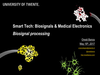
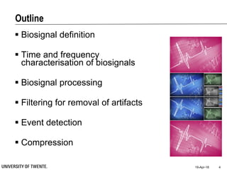
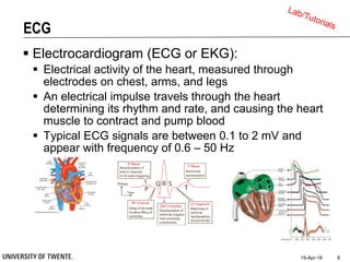
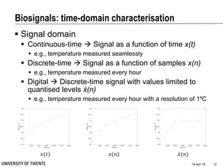
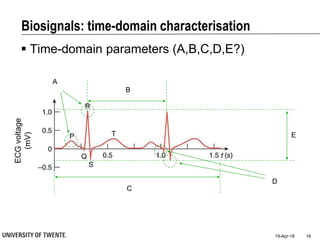
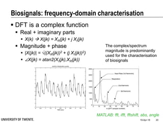
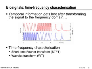
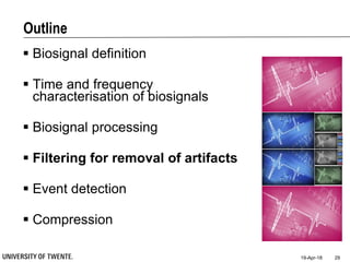
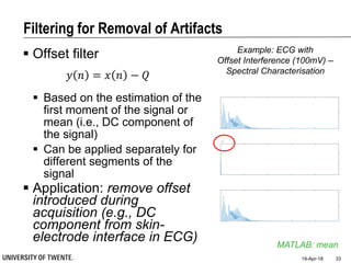
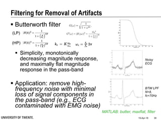
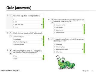
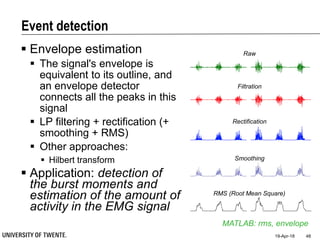
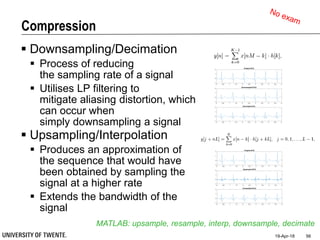
35. Filtering for Removal of Artifacts
 Median filter
 Ranks from lowest value to
highest value and picks the
middle one:
 e.g., median of [3, 3, 5, 9, 11] is 5
 Good for rejecting certain
types of noise in which some
samples take extreme values
(outliers)
 Application: regular power
source leading to ripples
riding on top of the signal
(e.g., power source
interference in ECG)
19-Apr-18 35
MATLAB: medfilt1
0 1 2 3 4 5
Time (s)
-1
0
1
2
ECG noisy signal and ideal signal
Noisy
Ideal
0 1 2 3 4 5
Time (s)
-1
0
1
2
ECG noisy signal and median-filtered signal
Noisy
medFiltered
0 1 2 3 4 5
Time (s)
-1
0
1
2
Median-filtered signal and ideal signal
medFiltered
Ideal
Example: ECG with
Powerline Interference (50Hz)

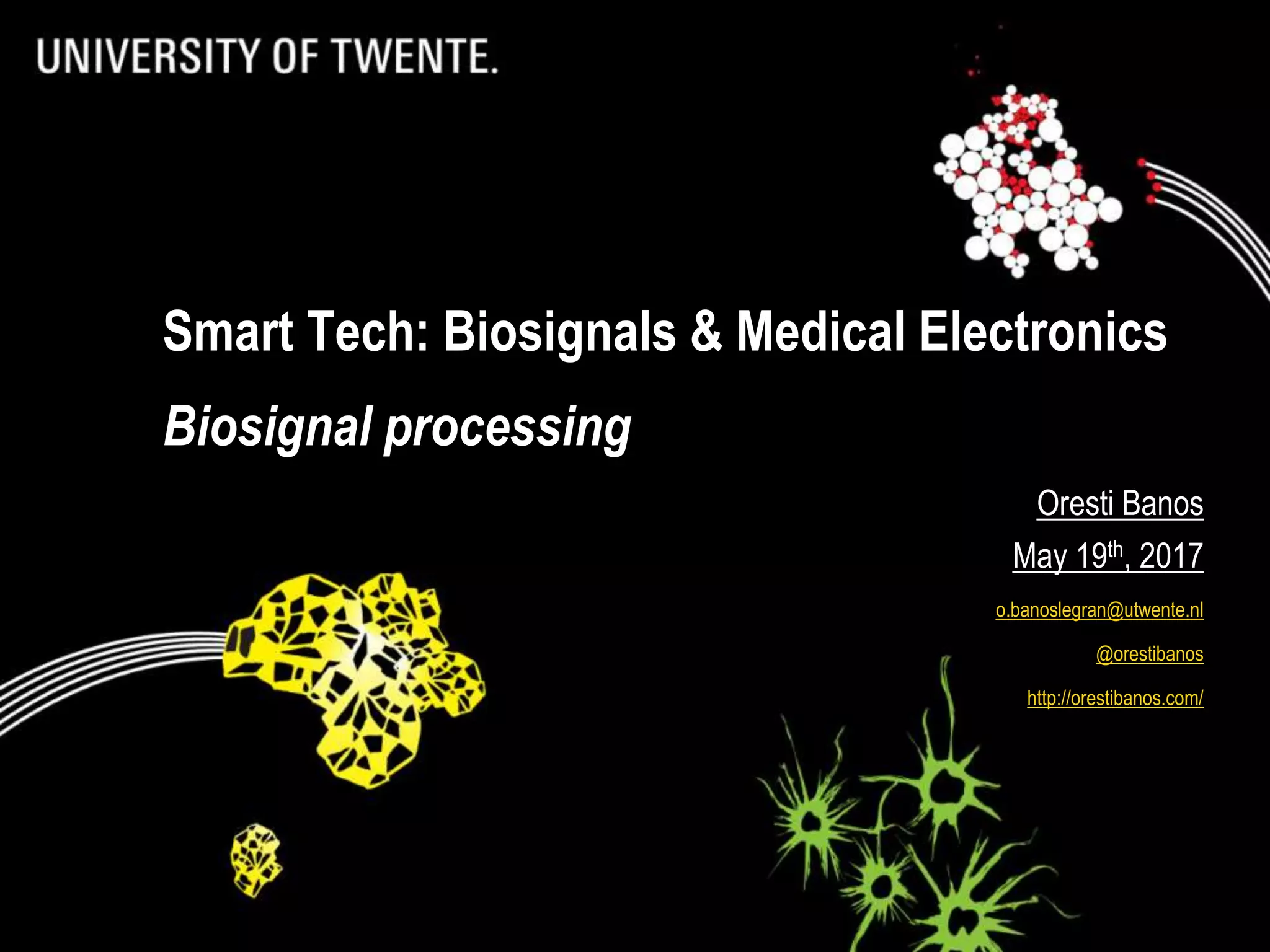
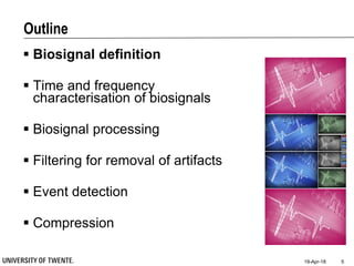
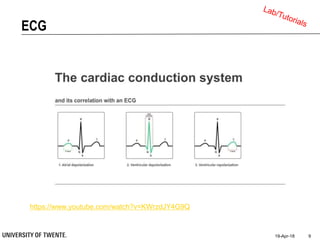
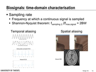
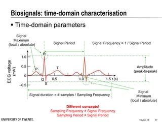
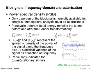
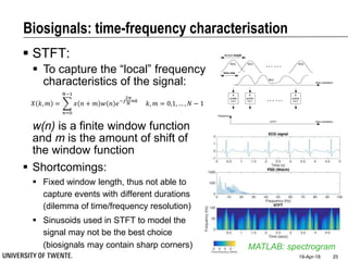
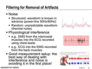
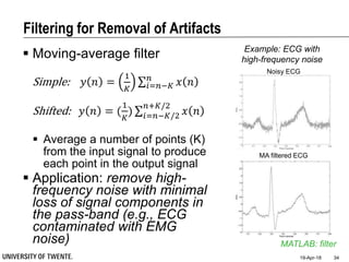
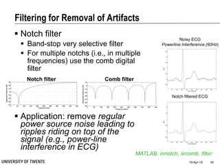
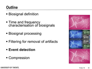
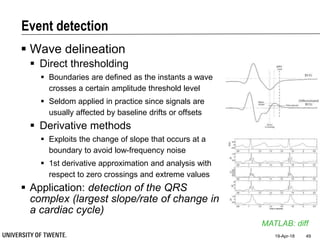
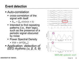
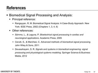
36. Filtering for Removal of Artifacts
 Median filter
 Ranks from lowest value to
highest value and picks the
middle one:
 e.g., median of [3, 3, 5, 9, 11] is 5
 Good for rejecting certain
types of noise in which some
samples take extreme values
(outliers)
 Application: regular power
source leading to ripples
riding on top of the signal
(e.g., power source
interference in ECG)
19-Apr-18 36
MATLAB: medfilt1
0 10 20 30 40 50 60 70 80 90 100
Frequency (Hz)
0
500
1000
PSD (ECG ideal)
0 10 20 30 40 50 60 70 80 90 100
Frequency (Hz)
0
500
1000
1500
PSD (ECG noisy)
0 10 20 30 40 50 60 70 80 90 100
Frequency (Hz)
0
500
1000
PSD (ECG filtered)
Example: ECG with
Powerline Interference (50Hz) –
Spectral Characterisation

37. Filtering for Removal of Artifacts
19-Apr-18 37
MATLAB: polyfit, polyval, detrend
Example: ECG baseline drift
(motion artifact)
0 0.5 1 1.5 2 2.5 3 3.5 4
Time (s)
-1
-0.5
0
0.5
1
1.5
2
Noisy ECG signal (base-line drift)
0 0.5 1 1.5 2 2.5 3 3.5 4
Time (s)
-1
-0.5
0
0.5
1
1.5
Detrended ECG signal
 Detrending filter
 Uses a polynomial
approximation based on
least-squares fit of a straight
line (or composite line for
piecewise linear trends) to
the signal
 Then subtracts the resulting
approximate function from
the original signal
 Application: trends/shifts
(low-frequency artifacts)
leading to improper
amplitudes (e.g.,
breathing in ECG)

38. Filtering for Removal of Artifacts
19-Apr-18 38
MATLAB: polyfit, polyval, detrend
Example: ECG baseline drift
(motion artifact) –
Spectral Characterisation
 Detrending filter
 Uses a polynomial
approximation based on
least-squares fit of a straight
line (or composite line for
piecewise linear trends) to
the signal
 Then subtracts the resulting
approximate function from
the original signal
 Application: trends/shifts
(low-frequency artifacts)
leading to improper
amplitudes (e.g.,
breathing in ECG)

39. Filtering for Removal of Artifacts
 Butterworth filter
 Simplicity, monotonically
decreasing magnitude response,
and maximally flat magnitude
response in the pass-band
 Application: remove high-
frequency noise with minimal
loss of signal components in
the pass-band (e.g., ECG
contaminated with EMG noise)
19-Apr-18 39
MATLAB: butter, maxflat, filter
Noisy
ECG
BTW LPF
N=8,
fc=70Hz
(LP)
(HP)

40. Filtering for Removal of Artifacts
 Notch filter
 Band-stop very selective filter
 For multiple notchs (i.e., in multiple
frequencies) use the comb digital
filter
 Application: remove regular
power source noise leading to
ripples riding on top of the
signal (e.g., power-line
interference in ECG)
19-Apr-18 40
MATLAB: iirnotch, iircomb, filter
Noisy ECG
Powerline Interference (60Hz)
Notch filtered ECG
Notch filter Comb filter

41. Filtering for Removal of Artifacts
 Savitzky–Golay smoothing filter
 Method of data smoothing based
on local least-squares polynomial
approximation
 Used to "smooth out" a noisy
signal whose frequency span
(without noise) is large
 Preserves characteristics such as
local maxima and minima and
peak width
 Application: trends/shifts (low-
frequency artifacts) leading to
improper amplitudes (e.g.,
breathing in ECG)
19-Apr-18 41
MATLAB: sgolayfilthttp://www-inst.eecs.berkeley.edu/~ee123/fa11/docs/SGFilter.pdf
0 0.5 1 1.5 2 2.5 3 3.5 4
Time (s)
-1
-0.5
0
0.5
1
1.5
Voltage(mV)
noisy ECG signal
0 0.5 1 1.5 2 2.5 3 3.5 4
Time (s)
-1
-0.5
0
0.5
1
Voltage(mV)
SG-filtered ECG signal

42. Quiz
 Go to go.voxvote.com
 Insert the code PIN: 99020
19-Apr-18 42

43. Quiz
19-Apr-18 43

44. Quiz (answers)
19-Apr-18 44

45. Outline
 Biosignal definition
 Time and frequency
characterisation of biosignals
 Biosignal processing
 Filtering for removal of artifacts
 Event detection
 Compression
19-Apr-18 45

46. Event detection
 Biomedical signals carry
signatures of physiological events
 The part of a signal related to a
specific event of interest is often
referred to as an epoch (e.g.,
QRS wave in ECG)
 Event detection techniques are
normally used in order to identify
epochs
19-Apr-18 46
 Once an event is identified, the corresponding
waveform may be segmented and characterised
in terms of time or frequency (e.g., peak-to-peak
amplitude, waveshape/morphology, time duration,
intervals between events, energy distribution,
spectral components, etc.)

47. Event detection
 Envelope estimation
 Wave delineation
 Peak detection
 Cross-correlation
 Auto-correlation
19-Apr-18 47

48. Event detection
 Envelope estimation
 The signal's envelope is
equivalent to its outline, and
an envelope detector
connects all the peaks in this
signal
 LP filtering + rectification (+
smoothing + RMS)
 Other approaches:
 Hilbert transform
 Application: detection of
the burst moments and
estimation of the amount of
activity in the EMG signal
19-Apr-18 48
MATLAB: rms, envelope
Raw
Filtration
Rectification
Smoothing
RMS (Root Mean Square)

49. Event detection
 Wave delineation
 Direct thresholding
 Boundaries are defined as the instants a wave
crosses a certain amplitude threshold level
 Seldom applied in practice since signals are
usually affected by baseline drifts or offsets
 Derivative methods
 Exploits the change of slope that occurs at a
boundary to avoid low-frequency noise
 1st derivative approximation and analysis with
respect to zero crossings and extreme values
 Application: detection of the QRS
complex (largest slope/rate of change in
a cardiac cycle)
19-Apr-18 49
MATLAB: diff

50. Event detection
 Peak detection
 Envelope estimation and
wave delineation are
frequently used in
combination
 Thresholding is used to
determine candidate peaks
 A local maxima search is
normally needed to select
outstanding peaks
 Application: estimation of
the ECG R-R distance
19-Apr-18 50
MATLAB: findpeaks

51. Event detection
 Peak detection
 Pan-Tomkins algorithm:
removing noise, smoothing
the signal, amplifying the
QRS slope and width, and
thresholding for detecting
peaks of interest
 Application: estimation of
the ECG R-R distance
19-Apr-18 51
MATLAB: filter, diff, rms, findpeaks

52. Event detection
 Cross-correlation
 Measures the similarity of
two series as a function of
the lag of one relative to
the other
 𝑅 𝑥𝑦 = 𝑛 𝑥 𝑛 𝑦(𝑛 + 𝑘)
 Intended to find common
patterns (i.e., their lags) in
a pair of signals
 Coherent Spectral Density
 𝐶𝑆𝐷 = 𝐷𝐹𝑇 𝑅 𝑥𝑦
 Application: detection of
EEG rhythms (⍺, β, δ, θ)
19-Apr-18 52
MATLAB: autocorr, xcorr

53. Event detection
 Auto-correlation
 cross-correlation of the
signal with itself
 𝑅 𝑥𝑥 = 𝑛 𝑥 𝑛 𝑥(𝑛 + 𝑘)
 Intended to find repeating
patterns (i.e., their lags),
such as the presence of a
periodic signal obscured
by noise
 Power Spectral Density
 𝑃𝑆𝐷 = 𝐷𝐹𝑇 𝑅 𝑥𝑦
 Application: detection of
EEG rhythms (⍺, β, δ, θ)
19-Apr-18 53
MATLAB: autocorr, xcorr

54. Outline
 Biosignal definition
 Time and frequency
characterisation of biosignals
 Biosignal processing
 Filtering for removal of artifacts
 Event detection
 Compression
19-Apr-18 54

55. Compression
 Process of reducing the amount of data in a given
signal to in order to lower resource usage, such
as data storage space or transmission capacity
 Sampling and quantisation are typical simple
compression techniques used to reduce the size
of the digitised signal
 Advantages:
 Less storage
 Less bandwidth
 Faster processing
 Disadvantages
 Information loss
19-Apr-18 55

56. Compression
 Downsampling/Decimation
 Process of reducing
the sampling rate of a signal
 Utilises LP filtering to
mitigate aliasing distortion, which
can occur when
simply downsampling a signal
 Upsampling/Interpolation
 Produces an approximation of
the sequence that would have
been obtained by sampling the
signal at a higher rate
 Extends the bandwidth of the
signal
19-Apr-18 56
MATLAB: upsample, resample, interp, downsample, decimate
0 0.5 1 1.5 2 2.5 3 3.5 4 4.5 5
-1
0
1
2
Original ECG
0 0.5 1 1.5 2 2.5 3 3.5 4 4.5 5
-1
0
1
2
Downsampled ECG
0 0.5 1 1.5 2 2.5 3 3.5 4 4.5 5
-1
0
1
2
Decimated ECG
0 0.5 1 1.5 2 2.5 3 3.5 4 4.5 5
-1
0
1
2
Original ECG
0 0.5 1 1.5 2 2.5 3 3.5 4 4.5 5
-1
0
1
2
Upsampled ECG
0 0.5 1 1.5 2 2.5 3 3.5 4 4.5 5
-1
0
1
2
Interpolated ECG

57. References
 Biomedical Signal Processing and Analysis:
 Principal reference:
 Rangayyan, R. M. Biomedical Signal Analysis: A Case-Study Approach. New
York: IEEE Press, 2002 (Chapters 1, 3, 4, 6)
 Other references:
 Sörnmo, L., & Laguna, P. Bioelectrical signal processing in cardiac and
neurological applications. Academic Press, 2005
 Cerutti, S., & Marchesi, C. Advanced methods of biomedical signal processing.
John Wiley & Sons, 2011
 Devasahayam, S. R. Signals and systems in biomedical engineering: signal
processing and physiological systems modeling. Springer Science & Business
Media, 2012
19-Apr-18 57

58. References
 Digital Signal Processing
 Principal reference:
 Proakis, J. G., & Manolakis, D. G. Digital Signal Processing. Principles,
Algorithms, and Applications. New Jersey: Prentice-Hall, 1996
 Other references:
 Hayes, M. Statistical Digital Signal Proccessing and Modeling. New York: John
Wiley & Sons, 1996
 [OPEN BOOK] Smith, Steven W., The Scientist and Engineer's Guide to Digital
Signal Processing, http://www.dspguide.com/pdfbook.htm
 [OPEN BOOK] Prandoni, P., Martin, V., Signal Processing for Communications,
http://www.sp4comm.org/docs/sp4comm_corrected.pdf
19-Apr-18 58

59. References
 Open database of physiological signals
(https://www.physionet.org/physiobank/database/)
19-Apr-18 59