Downloaded 2,574 times


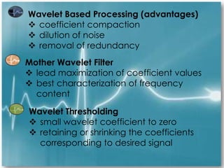


![ 3rd Step:
Determine the maximizer ym
OVERVIEW:
(7)- The incomplete elliptic integral
(9)- evaluated by the arithmetic-geometric mean [10].
Elliptic integral of the third kind P(x;y;k) in (10)
-evaluated by a fast procedure proposed in [7]](https://image.slidesharecdn.com/ecgfinaldraft-130924123930-phpapp01/85/Ecg-Signal-Processing-30-320.jpg)
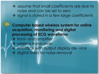
![NOTE:
no tool for the algebraic design of optimal
notch FIR filters
form of a Matlab function firnotch in Tab. 3
Purpose of tuning
adjust the actual notch frequency (fm to f0)
simplified version of the procedure introduced in [8]
Function Tune accepts:
impulse response h(k)
notch frequency fm[Hz] (initial filter)
desired notch frequency f0[Hz]
sampling frequency fs[Hz]](https://image.slidesharecdn.com/ecgfinaldraft-130924123930-phpapp01/85/Ecg-Signal-Processing-31-320.jpg)


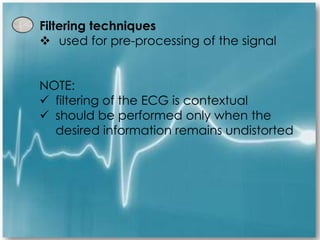
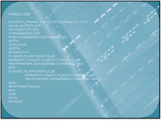
![function [n, h, f_m, adB_pass, adB_m]=firnotch(f_0, delta_f, fs, adB) %
Design
om_0_pi=2*pi*f_0/fs;
delom=2*pi*delta_f/fs;
om_0=om_0_pi/pi;
ym_s=-1+2/(1-10ˆ(0.05*adB));
omp=om_0_pi-delom/2; oms=om_0_pi+delom/2;
ws=cos(oms);
wp=cos(omp);
w_0=cos(om_0_pi);
fip=(pi-omp)/2;
fis=oms/2;
const=1/(tan(fis)*tan(fip));
k=sqrt(1-const*const);
quar=ellipke(k*k);
Ffis=ielli_fu(fis,k);
Ffip=ielli_fu(fip,k);
pn=Ffis/quar;
qn=Ffip/quar;
if fip==fis pn=0.5;
qn=0.5;
end](https://image.slidesharecdn.com/ecgfinaldraft-130924123930-phpapp01/85/Ecg-Signal-Processing-41-320.jpg)
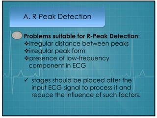
![n=degreez_fu(ym_s,pn,k,w_0,ws);
n=ceil(n);
p=round(pn*n);
q=round(qn*n);
[alph,wm]=zol_fu(p,q,k);
tm=alph;
tm=tm/2;
tm(1)=2*tm(1);
tp=fliplr(tm);
hn=[tp(1,1:max(size(tp))-1) tm];
om_m_pi=acos(wm);
om_m=om_m_pi/pi;
mazer=mag_fu(hn,[om_m_pi]);
if mazer<ym_s n=n+1;
p=round(pn*n);
q=round(qn*n);
[alph,wm]=zol_fu(p,q,k);
tm=alph;
tm=tm/2;
tm(1)=2*tm(1);
tp=fliplr(tm);
hn=[tp(1,1:max(size(tp))-1) tm];
om_m_pi=acos(wm);
om_m=om_m_pi/pi;
mazer=mag_fu(hn,[om_m_pi]);
end;](https://image.slidesharecdn.com/ecgfinaldraft-130924123930-phpapp01/85/Ecg-Signal-Processing-42-320.jpg)
![adB_pass=20*log10(1-2/(mazer+1));
tm=alph;
tm=tm/2;
tm(1)=2*tm(1);
tp=fliplr(tm);
hn=[tp(1,1:max(size(tp))-1) tm];
hn=-hn;
hn(1,1+floor(max(size(hn))/2))=mazer+hn(1,1+floor(max(size(hn))/2));
hn=hn/(1+mazer);
adB_m=20*log10(abs((mag_fu(hn,[om_m_pi]))));
f_m=om_m*fs/2;
h=hn; function y=Jacobi_Zeta_AGM_fu(u,k) % Jacobi Zeta function using AGM
sma=1e-12;
kc=sqrt(1-k*k);
a(1)=1;
b(1)=kc;
c(1)=k;
n=1;
while(c(n)>sma) n=n+1;
a(n)=0.5*(a(n-1)+b(n-1));
b(n)=sqrt(a(n-1)*b(n-1));
c(n)=0.5*(a(n-1)-b(n-1));
end;
fi(n)=(2ˆ(n-1))*a(n)*u; y=0;
for m = n:-1:2 cor=c(m)/a(m)*sin(fi(m));
fi(m-1)=0.5*(fi(m)+asin(cor));
y=y+c(m)*sin(fi(m));
end](https://image.slidesharecdn.com/ecgfinaldraft-130924123930-phpapp01/85/Ecg-Signal-Processing-43-320.jpg)


![function y=ellipi_fu(u,n,k) % Jacobi elliptic integral of third kind PI
quarter=ellipke(k*k);
si=ellipj(u,k*k);
s=ellipj((1:n)*quarter/n,k*k);
su=ellipj((1:n)*quarter/n+u,k*k);
sup=ellipj((1:n)*quarter/n-u,k*k);
v=u*k*k*s(1)*s(n-(1:n-1)).*s(n+1-(1:n-1));
num=1-k*k*s(1)*si*s(n-(1:n-1)).*sup(n+1-(1:n-1));
den=1+k*k*s(1)*si*s(n-(1:n-1)).*su(n+1-(1:n-1));
r=log(num./den)/2 + v;
a=diag(n-1:-1:1)*ones(n-1);
b=ones(n-1)-tril(ones(n-1));
y=flipud(1/n*(a-n*b)*r’);
function y=degreez_fu(ym,pn,k,wm,ws) % Degree of Zolotarev polynomial
cit=sqrt((wm-ws)/(wm+1));
quar=ellipke(k*k);
[sn,cn,dn]=ellipj(pn*quar,k*k);
jme=k*sn;
argu=asin(cit/jme);
sigmam=ielli_fu(argu,k);
pe=round(pn*1000);
eli3=ellipi_fu(sigmam,1000,k)’;
Pii=eli3(pe);
cit=log(ym+sqrt(ym*ym-1));
jme=2*sigmam*Jacobi_Zeta_AGM_fu(pn*quar,k)-2*Pii;
y=cit/jme;](https://image.slidesharecdn.com/ecgfinaldraft-130924123930-phpapp01/85/Ecg-Signal-Processing-46-320.jpg)
![function [a,wm]=zol_fu(p,q,km) % Zolotarev polynomial
n=p+q;
quarter=ellipke(km*km);
up=p*quarter/n;
[sn,cn,dn]=ellipj(up,km*km);
wp=2*(cn./dn)ˆ2-1;
ws=2*cnˆ2-1;
wm=ws+2*sn*cn/dn*Jacobi_Zeta_AGM_fu(up,km);
wq=(wp+ws)/2;
alfa=zeros(1,n+6);
alfa(n+1)=1;
for m=n+2:-1:3
c7=(n*n-(m-3)*(m-3))/8;
c6=((2*m-5)*(m-2)*(wm-wq)+3*wm*(n*n-(m-2)*(m- 2)))/4;
c5=3/8*(n*n-(m-1)*(m-1))+3/2*wm*(n*n*wm-(m-1)*(m- 1)*wq)-1/2*(m-
1)*(m-2)*(wp*ws-wm*wq);
c4=3/2*(n*n-m*m)*wm+m*m*(wm-wq)+wm*(n*n*wm*wm- m*m*wp*ws);
c3=3/8*(n*n-(m+1)*(m+1))+3/2*wm*(n*n*wm- (m+1)*(m+1)*wq)-
1/2*(m+1)*(m+2)*(wp*ws-wm*wq);
c2=((2*m+5)*(m+2)*(wm-wq)+3*wm*(n*n- (m+2)*(m+2)))/4; c1=(n*n-
(m+3)*(m+3))/8;](https://image.slidesharecdn.com/ecgfinaldraft-130924123930-phpapp01/85/Ecg-Signal-Processing-47-320.jpg)
![alfa(m-2)=(c6*alfa(m-1)-c5*alfa(m)+c4*alfa(m+1)- c3*alfa(m+2)+c2*alfa(m+3)-
c1*alfa(m+4))/c7;
end
alfa=[alfa(1)/2, alfa(2:n+1)];
suma=alfa(1);
for m=1:n
suma=suma+alfa(m+1);
end;
a=(-1)ˆp*alfa/suma;
function y=mag_fu(hn,om) % Magnitude of odd length FIR filter
nn=(max(size(hn))-1)/2;
y = hn(1+nn)*ones(max(size(om)),1);
for m=1:nn
y = y + 2*hn(nn+m+1)*cos(m*om);
end](https://image.slidesharecdn.com/ecgfinaldraft-130924123930-phpapp01/85/Ecg-Signal-Processing-48-320.jpg)
![tm(1)=2*tm(1);
tp=fliplr(tm);
h_t=[tp(1,1:max(size(tp))-1) tm];
function A_row=VectorA_fu(n,lambda,dir,row)
A_row=zeros(1,n+1);
if dir == 0 A_row(1:row)=tposun_fu(row-1,lambda, 1-lambda,-1);
elseif dir == 1 A_row(1:row)=tposun_fu(row-1,lambda, 1-lambda,1);
else A_row(1:row)=tposun_fu(row-1,1, 0, 1);
size(A_row);
end
function A=MatrixA_fu(n,lambda,dir)
for i=1:n+1
row=zeros(1,n+1);
A(i,:)=row;
end
if dir == 0 for i=1:n+1, aplus=tposun_fu(i-1,lambda, 1-lambda,-1);
A(i,1:i)=aplus;
end
elseif dir == 1 for i=1:n+1, aminus=tposun_fu(i-1,lambda,1-lambda,1);
A(i,1:i)=aminus;
end
else for i=1:n+1, aminus=tposun_fu(i-1,1,0,1);
A(i,1:i)=aminus;
end
end](https://image.slidesharecdn.com/ecgfinaldraft-130924123930-phpapp01/85/Ecg-Signal-Processing-50-320.jpg)
![function alfa=tposun_fu(n,lambda,lambdac,s)
if n==0, alfa(1)=1;
else alfa=zeros(1,n+4);
alfa(n+1)=lambdaˆn;
for k=1:1:n d1=k*(2*n-k);
d2=2*s*((k-1)*(2*n+1-k)-lambdac/lambda*(n+1-k)*(2*n+1-2*k));
d3=4*lambdac/lambda*(n+2-k);
d4=-2*s*((k-3)*(2*n+3-k)-lambdac/lambda*(n+3-k)*(2*n+7-2*k));
d5=(k-4)*(2*n+4-k);
alfa(n+1-k)=(alfa(n+2-k)*d2+alfa(n+3-k)*d3+alfa(n+4-k)*d4+alfa(n+5-k)*d5)/d1;
end
alfa=[alfa(1)/2 alfa(2:n+1)];
end](https://image.slidesharecdn.com/ecgfinaldraft-130924123930-phpapp01/85/Ecg-Signal-Processing-51-320.jpg)


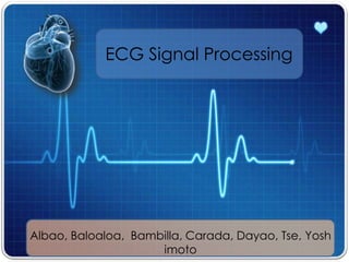
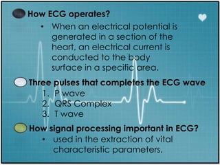
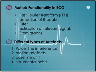
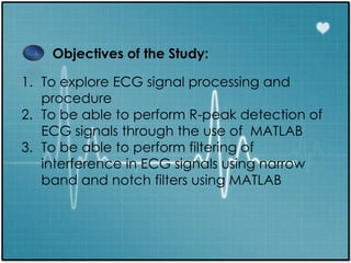
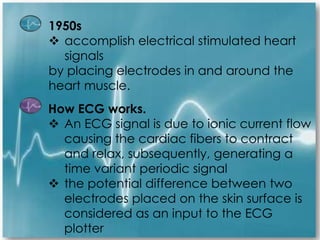
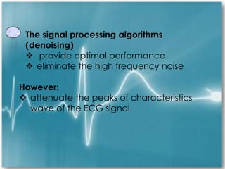
This document discusses ECG signal processing. It begins with an introduction to electrocardiograms and how they differ from EKGs. It then discusses how signal processing is important for ECGs and how ECGs operate based on three pulse waves. MATLAB functionality for ECG signal processing like FFTs and filtering is also covered. The document discusses various types of artefacts and noise sources that affect ECG signals. It outlines the objectives and methods of research which involve R-peak detection and notch filtering. Source code for these methods is also provided.