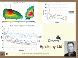
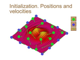
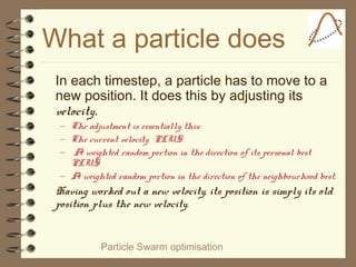
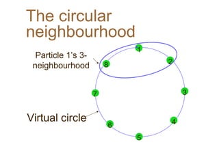
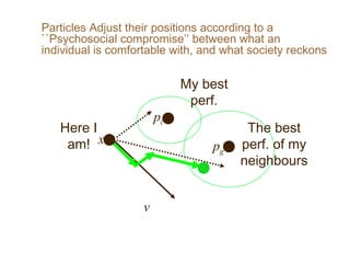
Particle Swarm Optimization (PSO) is an algorithm for optimization that is inspired by swarm intelligence. It was invented in 1995 by Russell Eberhart and James Kennedy. PSO optimizes a problem by having a population of candidate solutions, called particles, that fly through the problem space, with the movements of each particle influenced by its own best solution and the best solution in its neighborhood.


![Particle Swarm optimisation
Pseudocode
http://www.swarmintelligence.org/tutorials.php
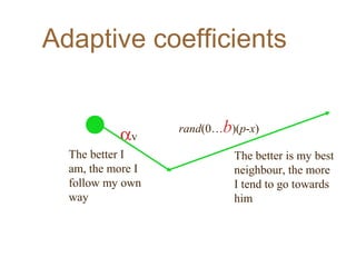
Equation (a)
v[] = c0 *v[]
+ c1 * rand() * (pbest[] - present[])
+ c2 * rand() * (gbest[] - present[])
(in the original method, c0=1, but many
researchers now play with this parameter)
Equation (b)
present[] = present[] + v[]](https://image.slidesharecdn.com/bicpso-150427141101-conversion-gate02/85/Bic-pso-13-320.jpg)


![... and some typical results
30D function PSO Type 1" Evolutionary
algo.(Angeline 98)
Griewank [±300] 0.003944 0.4033
Rastrigin [±5] 82.95618 46.4689
Rosenbrock [±10] 50.193877 1610.359
Optimum=0, dimension=30
Best result after 40 000 evaluations](https://image.slidesharecdn.com/bicpso-150427141101-conversion-gate02/85/Bic-pso-21-320.jpg)