The document describes the traveling salesman problem (TSP) and how to solve it using a branch and bound approach. The TSP aims to find the shortest route for a salesman to visit each city once and return to the starting city. It can be represented as a weighted graph. The branch and bound method involves reducing the cost matrix by subtracting minimum row/column values, building a state space tree of paths, and choosing the path with the lowest cost at each step. An example demonstrates these steps to find the optimal solution of 24 for a 5 city TSP problem.

1. Traveling Salesman Problem
• Problem Statement
– If there are n cities and cost of traveling from any
city to any other city is given.
– Then we have to obtain the cheapest round-trip
such that each city is visited exactly ones returning
to starting city, completes the tour.
– Typically travelling salesman problem is represent
by weighted graph.

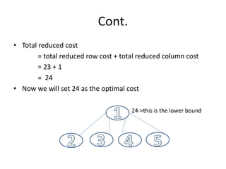
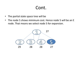
2. Cont.
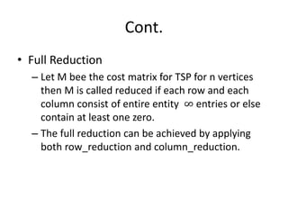
• Row Minimization
– To understand solving of travelling salesman
problem using branch and bound approach we
will reduce the cost of cost matrix M, by using
following formula.
– Red_Row(M) = [ Mij – min{ Mij | 1<=j<=n} ]
where Mij < ∞

3. Cont.
• Column Minimization
– Now we will reduce the matrix by choosing
minimum for each column.
– The formula of column reduction of matrix is
– Red_col(M)=Mij – min { Mij | 1<=j<=n}
where Mij < ∞

4. Cont.
• Full Reduction
– Let M bee the cost matrix for TSP for n vertices
then M is called reduced if each row and each
column consist of entire entity ∞ entries or else
contain at least one zero.
– The full reduction can be achieved by applying
both row_reduction and column_reduction.

5. Cont.
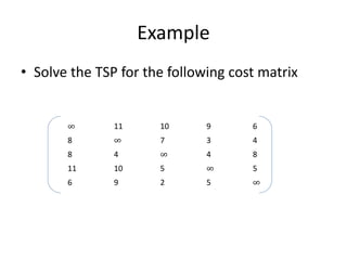
• Dynamic Reduction
– Using dynamic reduction we can make the choice of
edge i->j with optimal cost.
– Step in dynamic reduction technique
1. Draw a space tree with optimal cost at root node.
2. Obtain the cost of matrix for path i->j by making I row and
j column entries as ∞. Also set M[i][j]=∞
3. Cost corresponding node x with path I, j is optimal cost +
reduced cost+ M[i][j]
4. Set node with minimum cost as E-node and generate its
children. Repeat step 1 to 4 for completing tour with
optimal cost.

6. Example
• Solve the TSP for the following cost matrix
∞ 11 10 9 6
8 ∞ 7 3 4
8 4 ∞ 4 8
11 10 5 ∞ 5
6 9 2 5 ∞

7. Solution
Step 1 :
• We will find the minimum value from each row and
subtract the value from corresponding row
Minvalue
reduce matrix
∞ 11 10 9 6
8 ∞ 7 3 4
8 4 ∞ 4 8
11 10 5 ∞ 5
6 9 2 5 ∞
∞ 5 4 3 0
5 ∞ 4 0 1
4 0 ∞ 0 4
6 5 0 ∞ 0
1 4 0 0 ∞
-> 6
-> 3
->4
->5
->5
---------
23

8. Cont.
• Now we will obtain minimum value from each column. If they
column contain 0 the ignore that column and a fully reduced
matrix can be obtain.
subtracting 1 from 1st column
∞ 5 4 3 0
5 ∞ 4 0 1
4 0 ∞ 0 4
6 5 0 ∞ 0
1 4 0 0 ∞
∞ 5 4 3 0
4 ∞ 4 0 1
3 0 ∞ 0 4
5 5 0 ∞ 0
0 4 0 0 ∞

9. Cont.
• Total reduced cost
= total reduced row cost + total reduced column cost
= 23 + 1
= 24
• Now we will set 24 as the optimal cost
24->this is the lower bound

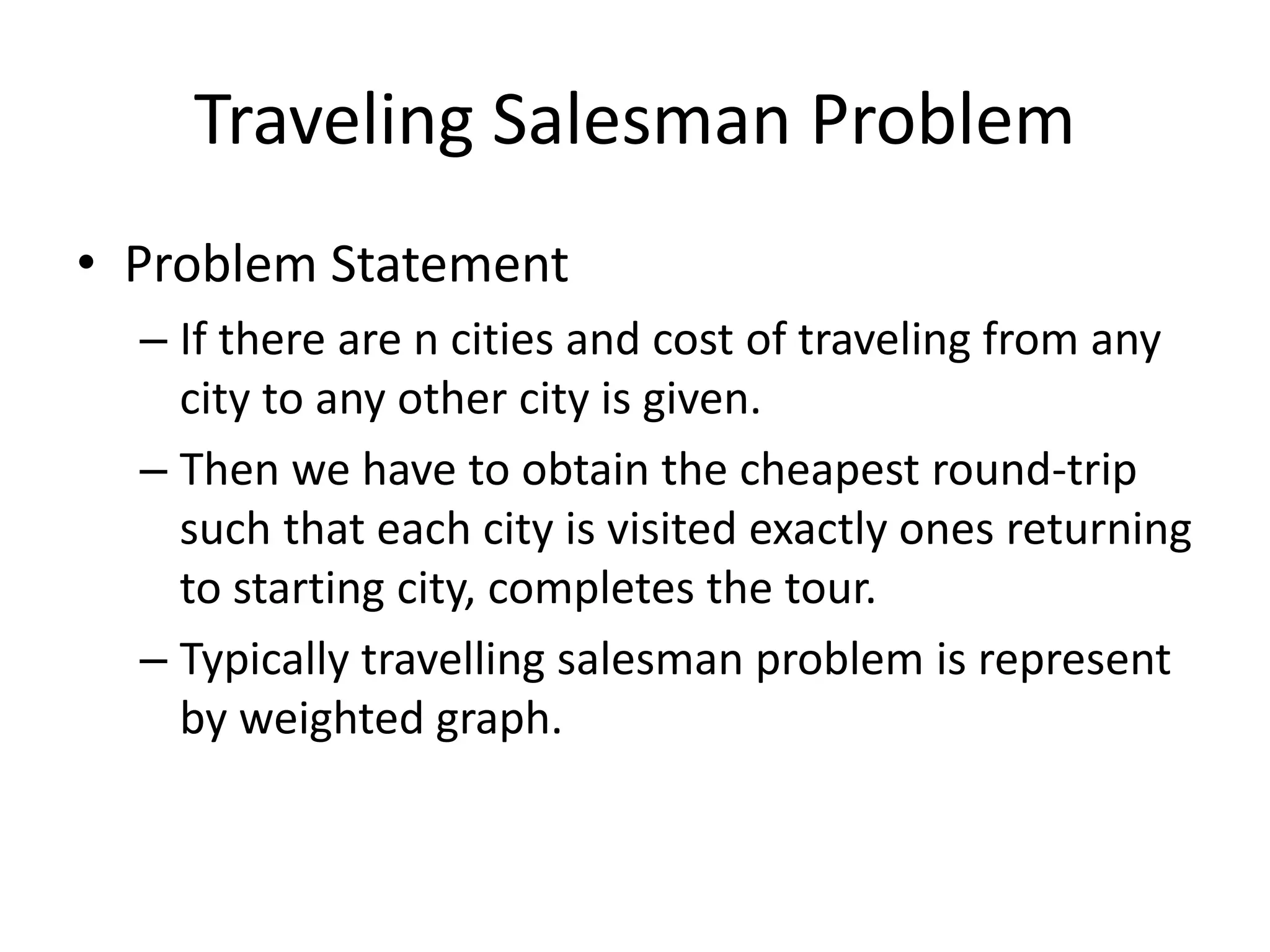
10. Cont.
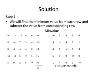
• Step 2 :: Now we will consider the paths [1,2], [1,3], [1,4] and [1,5] of state
space tree as given above consider path [1,2] make 1st row and 2nd column to
∞ set M[2][1]=∞
• Now we will find min value from each corresponding column.
• c
∞ ∞ ∞ ∞ ∞
∞ ∞ 4 0 1
3 ∞ ∞ 0 4
5 ∞ 0 ∞ 0
0 ∞ 0 0 ∞
∞ ∞ ∞ ∞ ∞
∞ ∞ 4 0 1
3 ∞ ∞ 0 4
5 ∞ 0 ∞ 0
0 ∞ 0 0 ∞

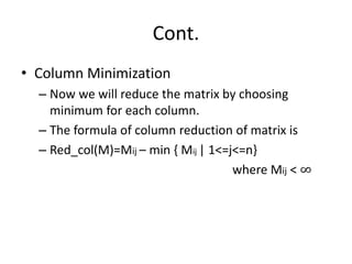
11. Cont.
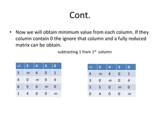
• Hence total receded cost for node 2 is = Optimal
cost+old value of M[1][2]
= 24 + 5
= 25
• Consider path (1,3). Make 1st row, 3rd column to be
∞ set M[3][1] = ∞

12. Cont.
There is no minimum value from any row and column
Hence total cost of node 3 is
= optimum cost + M[1][3]
= 24+ 4
= 28
∞ ∞ ∞ ∞ ∞
4 ∞ ∞ 0 1
3 0 ∞ 0 4
5 5 ∞ ∞ 0
0 4 ∞ 0 ∞

13. Cont.
• consider path [1,4] make 1st row and 4th column to ∞ set
M[4][1]=∞
subtracting 1 from 2nd Row
total cost of node 4 is = optimum cost + M[1][4] + minimum row cost
= 24+ 3+1
= 28
∞ ∞ ∞ ∞ ∞
4 ∞ 4 ∞ 1
3 0 ∞ ∞ 4
∞ 5 0 ∞ 0
0 4 0 ∞ ∞
∞ ∞ ∞ ∞ ∞
4 ∞ 3 ∞ 0
3 0 ∞ ∞ 4
∞ 5 0 ∞ 0
0 4 0 ∞ ∞

14. Cont.
• consider path [1,5] make 1st row and 5th column to ∞ set
M[5][1]=∞
subtracting 3 from 1st Row
total cost of node 5 is = reduced column cost + old value M[1][5]
= 24+ 3+0
= 27
∞ ∞ ∞ ∞ ∞
4 ∞ 4 0 ∞
3 0 ∞ 0 ∞
5 5 0 ∞ ∞
∞ 4 0 0 ∞
∞ ∞ ∞ ∞ ∞
1 ∞ 4 0 ∞
0 0 ∞ 0 ∞
2 5 0 ∞ ∞
∞ 4 0 0 ∞

15. Cont.
• The partial state space tree will be
• The node 5 shows minimum cost. Hence node 5 will be an E
node. That means we select node 5 for expansion.
27
29 28 28 27

16. Cont.
• Step 3 :: Now we will consider the paths [1,5,2], [1,5,3] and [1,5,4] of state
space tree as given above consider path [1,5,2] make 1st row , 5th row and
second column as ∞ set M[5][1] and M[2][1] =∞
subtracting 3 from 1st Column.
Hence total cost of node 6 is =optimal cost node 5+column reduced cost+ M[5][2]
= 27+ 3+4
= 34
∞ ∞ ∞ ∞ ∞
∞ ∞ 4 0 1
3 ∞ ∞ 0 4
5 ∞ 0 ∞ 0
∞ ∞ ∞ ∞ ∞
∞ ∞ ∞ ∞ ∞
∞ ∞ 4 0 1
0 ∞ ∞ 0 4
2 ∞ 0 ∞ 0
∞ ∞ ∞ ∞ ∞

17. Cont.