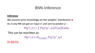
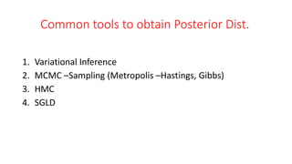
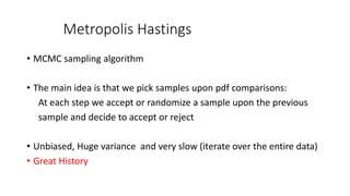
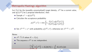
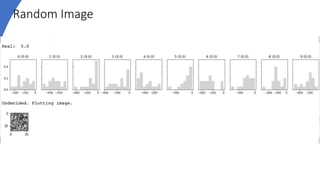
This document discusses Bayesian neural networks. It begins with an introduction to Bayesian inference and variational inference. It then explains how variational inference can be used to approximate the posterior distribution in a Bayesian neural network. Several numerical methods for obtaining the posterior distribution are covered, including Metropolis-Hastings, Hamiltonian Monte Carlo, and Stochastic Gradient Langevin Dynamics. Finally, it provides an example of classifying MNIST digits with a Bayesian neural network and analyzing model uncertainties.

1. Bayesian Neural Network
Natan Katz
Natan.katz@gmail.com

2. Agenda
• Short Introduction to Bayesian Inference
• Variational Inference
• Bayesian Neural Network
• Numerical Methods
• MNIST Example

3. Bayesian Inference

4. Bayesian Inference
The inputs:
Evidence – A Sample of observations (numbers, categories, vectors, images)
Hypothesis - An assumption about the prob. structure that creates the sample
Objective :
We wish to learn the optimal parameters of this distribution.
• This probability is called Posterior .
• We wish to find the optimal parameters for P(H|E)
• Remark In many books it is called MAP (Maximum A postriori Estimation)

5. Let’s Formulate
Z- R.V. that represents the hypothesis
X- R.V. that represents the evidence
Bayes formula:
P(Z|X) =
𝑃(𝑍,𝑋)
𝑃(𝑋)

6. Let’s Formulate (Cont.)
𝑃𝑟(Z) –Prior (The parameters’ distribution according to our belief)
𝑃𝑙(X|Z) –Likelihood (How likely is the sample given the parameters)
P(Z|X) =
𝑃𝑟(z) 𝑃 𝑙(x|z)
𝑃(𝑋)
Bayesian inference is therefore about working with the RHS terms.
In some case studying the denominator is intractable or extremely
difficult to calculate.

7. Example -GMM
We have K Gaussians with known variance σ
Draw μ 𝑘 ~ 𝑁 0, τ (τ is positive) from the prior
For each sample j =1…n
𝑧𝑗 ~Cat (1/K,1/K…1/K)
𝑥𝑗 ~ 𝑁(μ 𝑧 𝑗
, σ)
p(𝑥1….𝑛) = μ1:𝑘 𝑙=1
𝐾
𝑃(μ𝑙) 𝑖=1
𝑛
𝑧 𝑗
𝑝( 𝑧𝑗) P(𝑥𝑖|μ 𝑧 𝑗
) => 𝑃𝑟𝑒𝑡𝑡𝑦 𝑆ℎ𝑖𝑡

8. Some Good news
P(Z|X) =
𝑃𝑟(z) 𝑃 𝑙(x|z)
𝑃(𝑋)
• We wish to learn Z
• There is no Z in the denominator
=> P(Z|X) α 𝑃𝑙 𝑋 𝑍 𝑃𝑟(𝑍)

9. Solutions
Until 1999
Mostly numerical sampling:
• Metropolis Hastings
• RBM

10. Variational
Inference

11. “AN INTRODUCTION TO VARIATIONAL METHODS FOR GRAPHICAL MODELS”
11

12. VI – Algorithm Overview
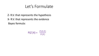
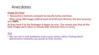
• Rather a numerical sampling method we provide an analytical one:
1. We define a distribution family Q(Z) (bias-variance trade off)
2. We minimize KL divergence min KL(Q(z)|| P(Z|X))
log(P(X)) = 𝐸 𝑄 [log P(x, Z)] − 𝐸 𝑄 [log Q(Z)] + KL(Q(Z)||P(Z|X))
ELBO-Evidence Lower Bound
• Maximizing ELBO =>minimizing KL

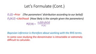
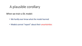
13. 𝐸𝐿𝐵𝑂 = 𝐸 𝑄[log P(X, Z)] − 𝐸 𝑄 [log Q(Z)] = 𝑄𝐿𝑜𝑔(
𝑃(𝑋,𝑍)
𝑄(𝑍)
)= J(Q)- Euler Lagrange
MFT (Mean Field Theory)
Scientific “approval”
13

14. What Deep Learning
doesn’t do

15. A DL Scenario
• We train a CNN to identify images (men versus women)
• Our accuracy can be amazing (98-99%)
Pretty cool

16. Let’s get Cruel
• We offer the model an image of a basketball
• The model outputs “man” or “woman”

17. Why is that?
Mathematical Observation
We trained a function F such that
F : {space of images}->{“man”,”woman”}
Statistical Observation
Basketball image is out of our training data

18. Anecdotes
Image (Uri Itay)
• Researchers trained a network to classify tanks and trees.
After using 200 images (100 of each kind 50 train 50 test), the test accuracy
was 100% .
As they took it to the Pentagon it began to miss. The reason was that all the
tank images were taken in cloudy days whereas trees in sunny.
Text
• We can see in text problems many cases where rather finding latent
phenomena networks use words as their anchor.

19. A plausible corollary
When we train a DL model:
• We hardly ever know what the model learned
• Models cannot “report” about their uncertainties

20. Is it crucial ?
• Consider an engine that decides upon AI whether a tumor is
malignant or benign
• Drug treatment upon medical record
• Actions that are taken by an autonomous vehicle
• High frequency trading

21. What can we do?
• DL models are trained to the optimal weights
• What if rather training weights pointwise, we ill train
weights’ distributions?
The Inference
• For each data pair (x,y) we create mean and variance
• This variance will reflect model’s uncertainty
• DL approach – Do Dropout in inference

22. Uncertainty Types
Epistemic Uncertainty :
Episteme= Knowledge
Uncertainty that theoretically we can know but we don’t:
• Model structure issues
• Absence of data
We can use the notion “reducible” too

23. Uncertainty Types
Aleatoric Uncertainty :
Aleator = Dice Player
Uncertainty that we cannot solve:
• The stochasticity of a dice
• Noisy labels
We can use the notion “irreducible” too

24. Bayesian Neural Network

25. BNN-Training
• We have a neural network
• We place a prior distribution P over the weights W
• For data D={ (X,Y)}
For measuring uncertainties, we use the posterior Distribution

26. DL Vs. BNN
DL
1. Training using a loss that is related to prediction probability P(Y|X,W)
2. The weights W are trained point-wise with MLE
Bayesian NN
1. Training using a loss that is related the posterior probability P(W|X,Y)
2. We train weights’ distribution

27. BNN-Inference
Inference
We assume prior knowledge on the weights’ distribution π
As in any NN we get an input x’ and aim to predict y’ :
P(y’| x’) = 𝑃 y’ 𝑥′
, 𝑤 𝑃 𝑤 𝐷 𝑑𝑤
This can be rewritten as:
P(y’| x’) =𝐸 𝑃(𝑤|𝐷) 𝑃 y’ 𝑥′
, 𝑤
D={(X,Y)}

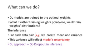
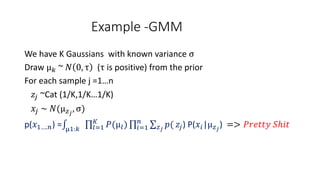
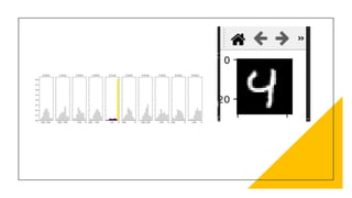
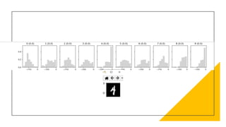
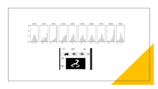
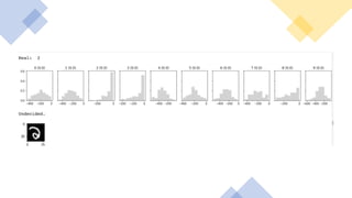
28. Measuring Uncertainty
• In the inference, given a data point 𝑥∗
• Sample weights W 𝑛 𝑡𝑖𝑚𝑒𝑠
• Calculate its statistics
E[f(𝑥∗
,w)]= 𝑖=1
𝑛
𝑓(𝑥∗
, 𝑤𝑖)
V([f(𝑥∗
,w)] =E𝑓(𝑥∗
,w)2
- E[f(𝑥∗
,w)]2
W –r.v. which 𝑤𝑖 is its samples

29. Common tools to obtain Posterior Dist.
1. Variational Inference
2. MCMC –Sampling (Metropolis –Hastings, Gibbs)
3. HMC
4. SGLD

30. Metropolis Hastings
• MCMC sampling algorithm
• The main idea is that we pick samples upon pdf comparisons:
At each step we accept or randomize a sample upon the previous
sample and decide to accept or reject
• Unbiased, Huge variance and very slow (iterate over the entire data)
• Great History

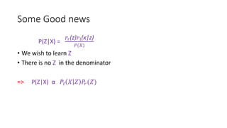
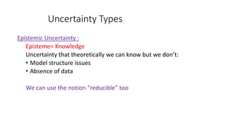
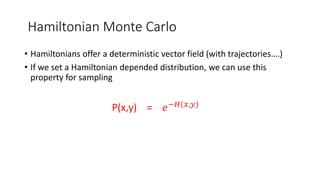
32. What is Hamiltonian?
• A physical operator that measures energy of a dynamical system
Two sets of coordinates
q -State coordinates
p- Momentum
H(p, q) =U(q) +K(p)
U(q) = log[π 𝑞 𝐿(𝑞|𝐷)] K(P)=
𝑝 2
2𝑚
U-Potential energy, K –Kinetic
𝑑𝐻
𝑑𝑝
= 𝑞 ,
𝑑𝐻
𝑑𝑞
= - 𝑝

33. Hamiltonian Monte Carlo
• Hamiltonians offer a deterministic vector field (with trajectories….)
• If we set a Hamiltonian depended distribution, we can use this
property for sampling
P(x,y) = 𝑒−𝐻(𝑥,𝑦)

34. Hybrid - MC
• We have the “state space” x
• We can add “momentum” and use Hamiltonian mechanism
Leap Frog Algorithm
We set a time interval δ, For each step i :
1. 𝑃𝑖(t+0.5 δ) =𝑃𝑖(t) – (δ/2)
𝑑𝑈
𝑑𝑞(𝑡)
2 𝑄𝑖(t+ δ ) = 𝑄𝑖(t) + δ
𝑑𝐾
𝑑𝑝(𝑡+0.5δ)
3 𝑃𝑖(t+ δ) = 𝑃𝑖(t+0.5 δ) - (δ/2)
𝑑𝑈
𝑑𝑞(𝑡+δ)
𝑄𝑖
𝑄

35. HMC
Algorithm (Neal 1995, 2012, Duane 1987)
1. Draw 𝑥0 from our prior
Draw 𝑝0 from standard normal dist.
2. Perform L steps of leapfrog
3 Pick the 𝑥 𝑡 following M.H.

37. HMC –Pros & Cons
Pros
• It takes points from a wider domains thus we can describe the
distribution better
• It may take points with lower density
• Faster than MCMC
Cons
• It may suffer from low energy barrier
• No minibatch –Not nice
• It has to calculate gradients for the entire data!!! Bad

38. What do we need then?
• A tool that allows sub-sampling
• Fewer Gradients
• Keen knowledge about extremums and escape rooms

39. Stochastic Gradient
Langevin Dynamics
(SGLD)

40. Langevin Equation
Langevin Equation describes the motion of pollen grain in water:
F -γ𝑣 𝑡 +ξ 𝑡=0 ξ 𝑡 ~N(0,t)
ξ 𝑡 is a Brownian Force- The collisions with the water molecules
F - External forces
This equation has an equilibrium solution which is our posterior
distribution

41. Langevin Equation
Let’s use the following:
F=𝛻𝐸 𝑣 𝑡 =
𝑑𝑋
𝑑𝑇
The eq in its discrete form becomes:
𝑥𝑡+1 = 𝑥𝑡 +
dt
γ
ξ 𝑡 + 𝛻𝐸
dt
γ
(looks familiar doesn’t it?)

42. Langevin Equation
Some more re-write:
𝑥𝑡+1 = 𝑥𝑡 + 𝜖 𝑡 𝛻𝐸 +ε 𝑡 ε 𝑡 -Stochastic term
Consider this term
Are we in a better situation ?

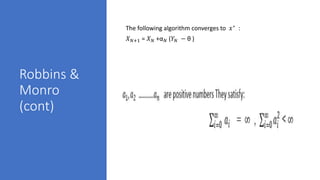
43. Robbins & Monro (Stoch. Approx. 1951)
• Let F a function and θ a number
• There exists a unique solution :
F(𝑥∗ ) = θ
F - is unknown
Y - A measurable r.v.
E[Y(x)] = F(x)

44. Robbins &
Monro
(cont)
The following algorithm converges to 𝑥∗ :
𝑋 𝑁+1 = 𝑋 𝑁 +α 𝑁 (𝑌𝑁 − θ )

45. Back to Langevin
𝑥 𝑡+1 = 𝑥 𝑡 + 𝜖 𝑡 𝛻𝐸 +ε 𝑡
𝛻𝐸 𝑚𝑏=𝛻𝐸 + ε 𝑡
𝑥 𝑡+1 = 𝑥 𝑡 + 𝜖 𝑡 𝛻𝐸 𝑚𝑏
Δ 𝜃𝑡 =ε 𝑡(𝛻log 𝑝 𝜃𝑡 +
𝑁
𝑛 𝑖=1
𝑁
𝛻log 𝑝 𝑥𝑖|𝜃𝑡 )

46. We are almost there
• This eq converges to an optimal solution (MAP).
• We need a solution of SDE (probability)
• Let’s add a stochastic term
Δ 𝜃𝑡 =ε 𝑡(𝛻log 𝑝 𝜃𝑡 +
𝑁
𝑛 𝑖=1
𝑁
𝛻log 𝑝 𝑥𝑖|𝜃𝑡 ) + η 𝑡 η 𝑡~N(0,σ)

47. Variance Analysis
ε 𝑡 - Follow R&M rules
How big is σ ?
Bigger than ε 𝑡 *V(𝛻)
As t->∞ the equation must become Langevin.
THE variance of η must be therefore bigger than ε 𝑡 *V(𝛻)

48. We do the
following:

49. Finally, Example
https://towardsdatascience.com/making-your-neural-network-say-i-
dont-know-bayesian-nns-using-pyro-and-pytorch-b1c24e6ab8cd

50. Problem’s Framework
• MNIST CNN model
• MNIST SOTA ~99.8%

51. The Experiment
• Training a BNN – using VI (small amount, of epochs)
• Set a regular decision law – Take the max score of each digit
=>Accuracy ~88%

52. Allowing the Network to refuse
• For each image:
• Sample 100 networks
• We obtain 100 outputs per image
• We have 10 digits each with 100 scores
• If the median of these 100 scores>0.2 we take
(Indeed, we can accept more than one result)

57. Random Image

58. Summary
• Accuracy 96%
• Refuse 12.5%
• Random images 95% have been refused

59. Thanks!!

60. My process
• https://wjmaddox.github.io/assets/BNN_tutorial_CILVR.pdf
• https://arxiv.org/pdf/2007.06823.pdf
• https://towardsdatascience.com/what-uncertainties-tell-you-in-bayesian-neural-networks-6fbd5f85648e
• https://medium.com/@uriitai/augmentation-and-groups-theory-795c287fec3f
• https://github.com/paraschopra/bayesian-neural-network-mnist/blob/master/bnn.ipynb
• https://towardsdatascience.com/making-your-neural-network-say-i-dont-know-bayesian-nns-using-pyro-
and-pytorch-b1c24e6ab8cd
• http://www.stats.ox.ac.uk/~teh/research/compstats/WelTeh2011a.pdf
• https://arxiv.org/pdf/1206.1901.pdf
• http://cgl.elte.hu/~racz/Stoch-diff-eq.pdf
• https://arxiv.org/ftp/arxiv/papers/1103/1103.1184.pdf
• https://henripal.github.io/blog/langevin
• https://www.cs.princeton.edu/courses/archive/fall11/cos597C/lectures/variational-inference-i.pdf