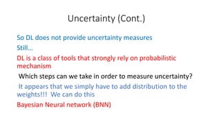
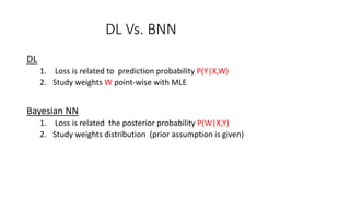
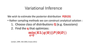
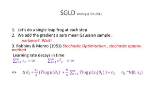
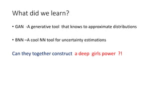
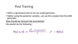
Generative adversarial networks (GANs) can be used to approximate the posterior distributions of Bayesian neural networks (BNNs). GANs are trained to generate samples from the posterior distribution learned by a BNN using stochastic gradient Langevin dynamics (SGLD). Specifically, a Wasserstein GAN with gradient penalty (WGAN-GP) is trained to match the posterior distribution by minimizing the Wasserstein distance between samples from the BNN's SGLD-approximated posterior and samples from the GAN's generator. This adversarial distillation technique allows parallel sampling from the BNN's posterior using only the GAN's parameters, providing computational and storage advantages over traditional Markov chain Monte Carlo methods for BNNs.

1. Gan with BNN

2. • Generative Models
• GAN –Foundation
• BNN
• GAN for BNN

3. What is Generative Models?
What it is not?
Discriminative models
• We study the conditional distribution P(Y=c|X=x)
c-class, x-features vector
• These models are trained for prediction tasks
• Most of the DL renaissance occurs in such models

4. Generative Model in Supervised Framework
Generative models Supervised
• We Train P(X=x| Y=c)
• By Bayes formula (and the prior on Y)we obtain the join dist P(Y,X)
We learn the statistical manners of a single class!!
We acquire the ability to generate samples from a given class
A common tool is Naïve Bayes

5. Generative Models (Cont)
Unsupervised
1. We don’t have target that guides us how to sectorize the data
2. We learn a generating deterministic function
x= f(z,θ)
f –deterministic, z –hidden variable θ -parameters
We aim to maximize the likelihood.

6. Before GAN
• Most of the generative models used sampling tools (M.H, Gibbs)
• Typically they need inference for next sampling (HMM, LDA,RBM)
• They suffer from several failure:
1. They don’t handle well high dimensions
2. Sampling converges slowly (they are “expensive”)
3. They prefer high distr domains, hence dont map the entire space
(M.H.)
4. Mini batch and gradient step are not always plausible.
Then came GAN

7. What was Adversarial?
Adversarial are simply perturbed inputs that may cause NN to
misclassify the data
1. They are often generated intentionally
2. They are located outside the data manifold (kind of noise)
Goodfellow -Explaining & Harnessing Adv. Ex.
He aimed to train DNN by introducing adversarial examples.

8. What is Adversarial now?
Nowadays
• Adversarial refers to a training on worst case scenario
examples
• One can think of it as a game between an agent and herself
Example : Samuels and his checker game ( 1950)
• GAN – The worst case scenario is created by a network too

9. Goodfellow’s Network
(pylearn2 code at https://github.com/goodfeli/adversarial)
Discriminator
A Common neural net (DNNCNN )
Input: a sample of real data
Output: The probability that the data is real data and not
“fake”
Labels: Simply 1 for real data and 0 for fake

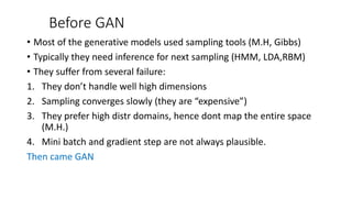
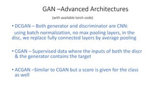
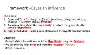
10. GAN
Generator
A Common neural net (DNN Goodfellow’s work)
Input: A generic distribution (GaussianUniform)
Output: Data sample from “real data” space such as fake images
Loss
𝒎𝒊𝒏
𝑮
𝒎𝒂𝒙
𝑫
(𝑽 𝑮, 𝑫 ) = 𝑬 𝒙~𝑷 𝒅𝒂𝒕𝒂(𝒙)[𝒍𝒐𝒈( 𝑫(𝒙))] + 𝑬 𝒛~𝑷(𝒛)[𝟏 − 𝒍𝒐𝒈( 𝑫(𝑮(𝒛))]

11. GAN –Advanced Architectures
(with available torch code)
• DCGAN – Both generator and discriminator are CNN:
using batch normalization, no max pooling layers, in the
disc, we replace fully connected layers by average pooling
• CGAN – Supervised data where the inputs of both the discr
& the generator contains the target
• ACGAN –Similar to CGAN but a score is given for the class
as well

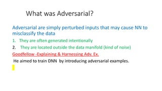
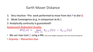
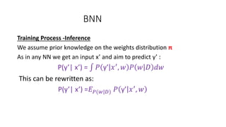
12. Wasserstein Distance
A distance between prob. Measures:
𝑊𝑝(𝜉, 𝜋) = min
𝛾∊𝛤
E[𝑑(𝑥, 𝑦) 𝑝 ]
ξ and π are the marginals of X and Y respectively
We discuss only 𝑊1 the Earth Mover Distance

13. Earth Mover Distance
1. Very intuitive –The work performed to move from dist P to dist Q
2. Weak Convergence (e.g. in comparison to KL )
3 Analytically continuity is guaranteed!!
Kantorovich-Rubinstein Duality:
𝑊 𝜉, 𝜋 = max
𝑓 𝐿 <1
𝐸 𝑋~𝜉 𝑓 𝑥 − 𝐸 𝑦~𝜋 𝑓 𝑦
• We can now train 𝑓 using a NN ( with some weights clipping to mimic the Lipschitz property)
• Arjovsky – Wassertein Gan

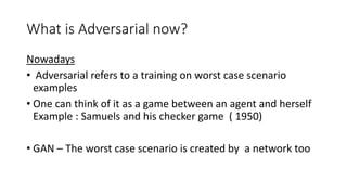
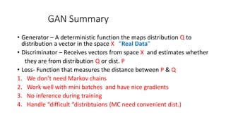
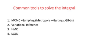
14. WGAN - GP
• As said Lipschitz property has not fully achieved
Gulrajani, Arjovsky Improved WGAN “WGAN-GP”
Rather weights clipping we add gradient penalty
L= 𝐸 𝑋~𝜉 𝐷 𝑥 − 𝐸 𝑦~𝜋 [𝐷 𝑦 ]+λ𝐸𝑧 [( 𝛻z 𝐷(𝑧) 2−1)2]
z =𝜀𝑥 + (1 − 𝜀) 𝑦 𝜉, 𝜋 Distributions
𝜀 ~ U[0,1]

15. GAN Summary
• Generator – A deterministic function the maps distribution Q to
distribution a vector in the space X “Real Data”
• Discriminator – Receives vectors from space X and estimates whether
they are from distribution Q or dist. P
• Loss- Function that measures the distance between P & Q
1. We don’t need Markov chains
2. Work well with mini batches and have nice gradients
3. No inference during training
4. Handle “difficult “distribtuions (MC need convenient dist.)

16. Uncertainty
• Statistics prediction tools such as Bayesian inference output
a confidence estimation in addition to the prediction score .
What about DL and confidence….?
Not too much … 

17. Uncertainty Types
Uncertainty Types:
1. Epistemic -Uncertainty due to lack of knowledge
Episteme= Knowledge
2. Aleatoric -Uncertainty due to noisy data :
We need better data not more data
Aleatory=dice player
The notions “reducible” & “irreducible” are used too

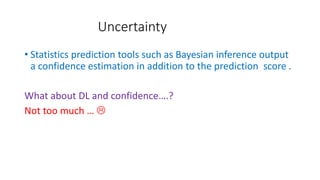
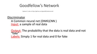
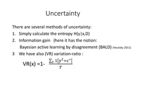
18. Uncertainty Estimation Methods
1. Conditional entropy:
H(P(y|x)) = 𝑦∈𝑌 𝑃(𝑦|𝑥) log 𝑃 𝑦 𝑥
Entropy can’t differentiate between epistemic & aleatoric uncertainty
2. Inform. Gain (info gain over params values upon input prediction)
I(w,y |x,D) =H[p(y|x, D)]- 𝐸 𝑝 𝑤 𝐷 𝐻[𝑝 𝑦 𝑥, 𝑤 ]
It well measures the epistemic uncertainty because little info implies that
the parameter is well known
3. (VR) variation-ratio :
VR(x) =1- 𝒕 𝟏 𝒚 𝒕=𝒄∗
𝑻

19. DL & Uncertainty
• Deep Learning does not handle confidence:
The network is trained to get features and returns probabilities or
numbers, but nothing about how certain the output is.
DL is about training deterministic functions upon data!!
Is uncertainty important ?
Images of dogs and cats are nice anecdote, but … What about MRI?
Melanoma?

21. Uncertainty (Cont.)
So DL does not provide uncertainty measures
Still…
DL is a class of tools that strongly rely on probabilistic
mechanism
Which steps can we take in order to measure uncertainty?
It appears that we simply have to add distribution to the
weights!!! We can do this
Bayesian Neural network (BNN)

22. DL Vs. BNN
DL
1. Loss is related to prediction probability P(Y|X,W)
2. Study weights W point-wise with MLE
Bayesian NN
1. Loss is related the posterior probability P(W|X,Y)
2. Study weights distribution (prior assumption is given)

23. Framework –Bayesian Inference
The inputs:
1. Observed Data D of length n ,{(x, y)} , (numbers, categories, vectors,
images) It is known also as–Evidence
2. An assumption about the probabilistic structure that generates the
sample –Hypothesis
3. Prior distribution - a pre-assumption about the hypothesis distribution
Objective :
• GainUpdate information about the Hypothesis using the Evidence
• We assume the Prior Prior and learn the Posterior P(H|D) .
• Bayes Formumla

24. BNN
Training Process -Inference
We assume prior knowledge on the weights distribution π
As in any NN we get an input x’ and aim to predict y’ :
P(y’| x’) = 𝑃 y’ 𝑥′
, 𝑤 𝑃 𝑤 𝐷 𝑑𝑤
This can be rewritten as:
P(y’| x’) =𝐸 𝑃(𝑤|𝐷) 𝑃 y’ 𝑥′
, 𝑤

25. Common tools to solve the integral
1. MCMC –Sampling (Metropolis –Hastings, Gibbs)
2. Variational Inference
3. HMC
4. SGLD

26. Variational Inference
We wish to estimate the posterior distribution P(Θ|D)
• Rather sampling methods we can construct analytical solution :
1. Choose class of distributions Q (e.g. Gaussians)
2. Find the q that optimizes:
𝐦𝐢𝐧
𝒒∊𝑸
(𝑲𝑳(𝒒(Θ)||𝑷(Θ|𝑫))
(Jordan ,1999 , Blei 2003, Graves 2011)

28. What is Hamiltonian?
• Operator that measures the total energy of an system
Two sets of coordinates
q -State coordinates (generalized coordinates)
p- Momentum
H(p, q) =U(q) +K(p)
U(q) = log[π 𝑞 𝐿(𝑞|𝐷)] K(P)=
𝑝 2
2𝑚
U-Potential energy, K –Kinetic
𝑑𝐻
𝑑𝑝
= 𝑞 ,
𝑑𝐻
𝑑𝑞
= - 𝑝

29. Hamiltonian Monte Carlo
Hamiltonians satisfy the following properties
1. They are Volume preserved (Liouville’s Theorem)
2. Time invariant
3. Time reversible
4. Hamiltonians offer a deterministic vector field (with trajectories….)
We can therefore use it for sampling needs, if we take distribution
that depends solely in the Hamiltonian!!
P(x,y) = 𝑒−𝐻(𝑥,𝑦)

30. Hybrid - MC
• We have the “state space” x
• We can add “momentum” and use Hamiltonian mechanism
Leap Frog Algorithm
We set a time interval δ, For each step i :
1. 𝑃𝑖(t+0.5 δ) =𝑃𝑖(t) – (δ/2)
𝑑𝑈
𝑑𝑞(𝑡)
2 𝑄𝑖(t+ δ ) = 𝑄𝑖(t) + δ
𝑑𝐾
𝑑𝑝(𝑡+0.5δ)
3 𝑃𝑖(t+ δ) = 𝑃𝑖(t+0.5 δ) - (δ/2)
𝑑𝑈
𝑑𝑞(𝑡+δ)
𝑄𝑖
𝑄

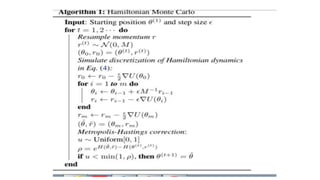
31. HMC
Algorithm (Neal 1995, 2012, Duane 1987)
1. Draw 𝑥0 from our prior
Draw 𝑝0 from standard normal dist.
2. Perform L steps of leapfrog
3 Pick the 𝑥 𝑡 upon M.H step
min [ 1, exp(−U(q ∗ ) + U(q) − K(p ∗ ) + K(p))]

33. HMC –Pros & Cons
Pros
• It takes points from a wider domains therefore we can describe the
distribution better and converges faster
• It may take points with lower density
• Faster than MCMC
• Ergodicity
Cons
• It may suffer from low energy barrier
• No minibatch
• It has to calculate gradients for the entire data!!! Bad

34. What do we need then?
• A tool that allows sub-sampling
• Fewer Gradients
• Keen knowledge about extremums and escape rooms

35. Langevin Equation
Langevin Equation describes the motion of pollen grain in water:
F -γ𝑣 𝑡 +ξ 𝑡=0 ξ 𝑡 ~N(0,I)
ξ 𝑡 is a Brownian Force- The collisions with the water molecules
We have : F=𝛻𝐸 𝑣 𝑡 =
𝑑𝑋
𝑑𝑇
=> 𝑥 𝑡+1 = 𝑥 𝑡 +
dt
γ
ξ 𝑡 + 𝛻𝐸
dt
γ
(looks familiar doesn’t it?)

36. SGLD Welling & Teh 2011
1. Let’s do a single leap frog at each step
2. We add the gradient a zero mean Gaussian sample .
variance? Wait!
3. Robbins & Monro (1951) Stochastic Optimization , stochastic approx.
method
Learning rate decays in time
𝑖=1
∞
ε 𝑡 = ∞ 𝑖=1
∞
ε2
𝑡 < ∞
=> Δ 𝜃𝑡 =
ε𝑡
2
(𝛻log 𝑝 𝜃𝑡 +
𝑁
𝑛 𝑖=1
𝑁
𝛻log 𝑝 𝑥𝑖|𝜃𝑡 ) + η 𝑡 η 𝑡 ~N(0, ε 𝑡)

37. What did we learn?
• GAN -A generative tool that knows to approximate distributions
• BNN –A cool NN tool for uncertainty estimations
Can they together construct a deep girls power ?!

38. GAN meets BNN
Adversarial Distillation of Bayesian Neural Network Posteriors
Basic Idea
• Train GAN to create posterior distribution of BNN
• We use WGAN-GP as loss function:
L = 𝑬 𝜭~𝑷 𝜭
[𝑫(θ)] -𝑬 𝝃~𝑷 𝒓
[𝑫(𝝃)] + λ 𝑬 𝜭~𝑷 𝜭
(〖 𝜵𝑫 θ 𝟐〗 − 𝟏) 𝟐
Two Steps Training
1. Create sample from the posterior using SGLD mechanism
2. Train the WGAN-GP to sample from this posterior

39. Adversarial Posterior Distillation (APD)
• A generative model that distills the posterior dist (P(θ|X)
Algorithmic advantage
1. Sample can be performed in parallel (MCMC is sequential)
2. A relatively small storage is required for the generator’s parameters

40. APD –Offline
1 Sample a series of weights: θ 𝑡 𝑡=1
𝑇
2 Optimize G using WGAN-GP , where θ 𝑡 𝑡=1
𝑇
is the
“real data
Remark: They used different version of SGLD
Baysian Dark Knowledge (2014,Murphy Welling)

41. APD -Online
1. Draw the θ 𝑡 using the Generator
2. Loop until convergence
• Draw θ 𝑡 upon MCMC method (Gibbs MH) for several iterations
• Put the samples in a buffer
• Use the buffer to optimize G where θ 𝑡 is the “real data”

42. Post Training
• GAN is a generative tool so we can simply generate….
• Rather using the posterior samples , we use the samples that the GAN
generates
How should we measure the uncertainty?
We predict by the following :
P(y| x, D) ≈ 𝑖=1
𝑇
𝑃(𝑦|𝑥,𝐺(𝑧 𝑡)
𝑇
𝑧 𝑡
~ N(0,I)

43. Uncertainty
There are several methods of uncertainty:
1. Simply calculate the entropy H(y|x,D)
2. Information gain (here it has the notion:
Bayesian active learning by disagreement (BALD) (Houlsby 2011)
3 We have also (VR) variation-ratio :
VR(x) =1- 𝑡 1 𝑦 𝑡=𝑐∗
𝑇

44. Some outcomes
• APD can retain SGLD features:
1. Anomaly detection
2. Defense
3. Active Learning
• APD reduces the storage cost of SGLD (or any other MCMC)
• WGAN-GP works better than Wasserstein or the original GAN

45. That’s All
THANKS!!!

46. • https://henripal.github.io/blog/langevin
• http://www.quretec.com/u/vilo/edu/2003-04/DM_seminar_2003_II/Bayes/lampinen01bayesian.pdf
• http://bayesiandeeplearning.org/2016/slides/nips16bayesdeep.pdf
• https://pdfs.semanticscholar.org/b0f2/433c088591d265891231f1c22424047f1bc1.pdf?_ga=2.47068911.9935516.1543231280-
34044526.1542095209
• https://arxiv.org/pdf/1505.05424.pdf
• https://henripal.github.io/blog/langevin -pytorch code
• https://www.coursera.org/lecture/bayesian-methods-in-machine-learning/bayesian-neural-networks-HI8ta
• https://pdfs.semanticscholar.org/49c6/c08709d3cbf4b58477375d7c04bcd4da4520.pdf
• https://pdfs.semanticscholar.org/579d/308b610da58266dbfa3574ba9c234ff1da13.pdf
• https://arxiv.org/pdf/1701.07875.pdf
• https://arxiv.org/pdf/1704.00028.pdf
• https://arxiv.org/pdf/1806.10317.pdf
• https://arxiv.org/abs/1112.5745

47. • https://www.ics.uci.edu/~welling/publications/papers/stoclangevin_v6.pdf
• https://www.cs.ox.ac.uk/people/yarin.gal/website/thesis/thesis.pdf
• http://arogozhnikov.github.io/2016/12/19/markov_chain_monte_carlo.html
• https://theclevermachine.wordpress.com/2012/11/18/mcmc-hamiltonian-monte-carlo-a-k-a-hybrid-monte-carlo/
• https://arxiv.org/pdf/1206.1901.pdf
• https://pdfs.semanticscholar.org/49c6/c08709d3cbf4b58477375d7c04bcd4da4520.pdf
• http://citeseerx.ist.psu.edu/viewdoc/download?doi=10.1.1.446.9306&rep=rep1&type=pdf
• https://papers.nips.cc/paper/4329-practical-variational-inference-for-neural-networks.pdf
• https://www.cs.toronto.edu/~graves/nips_2011.pdf
• https://arxiv.org/pdf/1206.1901.pdf
• https://danieltakeshi.github.io/2017/11/26/basics-of-bayesian-neural-networks/
• https://www.math.wustl.edu/~sawyer/hmhandouts/MetropHastingsEtc.pdf
• http://edwardlib.org/tutorials/bayesian-neural-network -code python
• http://physics.gu.se/~frtbm/joomla/media/mydocs/LennartSjogren/kap6.pdf
• https://www.ics.uci.edu/~welling/publications/papers/stoclangevin_v6.pdf
• https://henripal.github.io/blog/langevin
• https://pdfs.semanticscholar.org/34dd/d8865569c2c32dec9bf7ffc817ff42faaa01.pdf