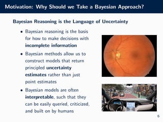
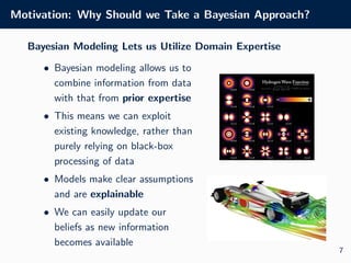
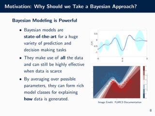
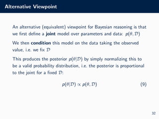
The document outlines the visual identity guidelines for the University of Oxford's logo and provides details for a machine learning course taught by Dr. Tom Rainforth. It includes information on coursework, assessments, lecture topics covering Bayesian machine learning, and explains key concepts in machine learning, including supervised and unsupervised learning. Furthermore, it emphasizes the importance of Bayesian methods in making decisions under uncertainty and provides insights into generative versus discriminative models.

1. 5
At the heart of our visual identity is the Oxford logo.
It should appear on everything we produce, from
letterheads to leaflets and from online banners to
bookmarks.
The primary quadrangle logo consists of an Oxford blue
(Pantone 282) square with the words UNIVERSITY OF
OXFORD at the foot and the belted crest in the top
right-hand corner reversed out in white.
The word OXFORD is a specially drawn typeface while all
other text elements use the typeface Foundry Sterling.
The secondary version of the Oxford logo, the horizontal
rectangle logo, is only to be used where height (vertical
space) is restricted.
These standard versions of the Oxford logo are intended
for use on white or light-coloured backgrounds, including
light uncomplicated photographic backgrounds.
Examples of how these logos should be used for various
applications appear in the following pages.
NOTE
The minimum size for the quadrangle logo and the
rectangle logo is 24mm wide. Smaller versions with
bolder elements are available for use down to 15mm
wide. See page 7.
The Oxford logo
Quadrangle Logo
Rectangle Logo
This is the square
logo of first
choice or primary
Oxford logo.
The rectangular
secondary Oxford
logo is for use only
where height is
restricted.
Lecture 1: Machine Learning Paradigms
Advanced Topics in Machine Learning
Dr. Tom Rainforth
January 22nd, 2020
rainforth@stats.ox.ac.uk

2. Course Outline
• Slightly unusual course covering different topics in machine
learning
• Aim is to get you interacting with actual research
• Fully assessed by coursework
• There are no examples sheets: you are instead expected to
take the initiative to investigate areas you find interesting and
familiarize yourself will software tools (we will suggest
resources and the practicals are there to help with software
familiarity)
1

3. Course Structure
• 6 lectures on Bayesian Machine Learning from me
• 8 lectures on Natural Language Processing from Dr Alejo
Nevado-Holgado
• A few guest lectures at the end
• Many of the lectures we be delivered back-to-back (e.g. I will
effectively give 2x1 hour lectures and 2x2 hour lectures)
2

4. Course Assessment
• Team project working in groups of 4
• Based on reproducing a research paper
• Each team has a different paper
• Produce a group report + statement of individual
contributions + poster
• Individual oral vivas
• Groups will be assigned by department, details are still being
sorted
• Check online materials—may end up being some tweaks
before you start
3

5. Bayesian Machine Learning—Course Outline
Lectures
• Machine Learning Paradigms (1 hour)
• Bayesian Modeling (2 hours)
• Foundations of Bayesian Inference (1 hour)
• Advanced Inference Methods (1 hour)
• Variational Auto-Encoders (1 hour)—key lecture for
assessments!
I will upload notes after each lecture. These will not perfectly
overlap with the lectures/slides so you will need to separately
digest each
4

6. What is Machine Learning?
Arthur Samuel, 1959
Field of study that gives computers the ability to learn without
being explicitly programmed.
Tom Mitchell, 1997
Any computer program that improves its performance at some task
through experience.
Kevin Murphy, 2012
To develop methods that can automatically detect patterns in
data, and then to use the uncovered patterns to predict future
data or other outcomes of interest.
5

7. Motivation: Why Should we Take a Bayesian Approach?
Bayesian Reasoning is the Language of Uncertainty
• Bayesian reasoning is the basis
for how to make decisions with
incomplete information
• Bayesian methods allow us to
construct models that return
principled uncertainty
estimates rather than just
point estimates
• Bayesian models are often
interpretable, such that they
can be easily queried, criticized,
and built on by humans
Medical Diagnostics
nopathy Diagnostics
nally:
n relies on expert confidence in
g medical record ! advises patient
reatment
arning:
dical record is unlike prev seen !
tem guesses at random, biases expert 6

8. Motivation: Why Should we Take a Bayesian Approach?
Bayesian Modeling Lets us Utilize Domain Expertise
• Bayesian modeling allows us to
combine information from data
with that from prior expertise
• This means we can exploit
existing knowledge, rather than
purely relying on black-box
processing of data
• Models make clear assumptions
and are explainable
• We can easily update our
beliefs as new information
becomes available
7

9. Motivation: Why Should we Take a Bayesian Approach?
Bayesian Modeling is Powerful
• Bayesian models are
state-of-the-art for a huge
variety of prediction and
decision making tasks
• They make use of all the data
and can still be highly effective
when data is scarce
• By averaging over possible
parameters, they can form rich
model classes for explaining
how data is generated.
Image Credit: PyMC3 Documentation
8

10. Learning From Data
8

11. Learning from Data
• Machine learning is all about learning from data
• There is generally a focus on making predictions at unseen
datapoints
• Starting point is typically a dataset—we can delineate
approaches depending on type of dataset
9

12. Supervised Learning
• We have access to a labeled dataset of input–output pairs:
D = {xn, yn}N
n=1.
• Aim is to learn a predictive model f that takes an input
x ∈ X and aims to predict its corresponding output y ∈ Y.
• The hope is that these example pairs can be used to “teach”
f how to accurately make predictions.
10

13. Supervised Learning—Classification
Classification
Cat
Cat
Classification
Cat
Dog
Classification
Cat
Flying
Spaghetti
Monster
Input x Predictor f (x) Class label y
11

14. Supervised Learning—Regression
12

15. Supervised Learning
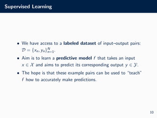
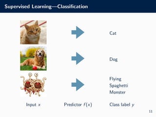
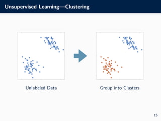
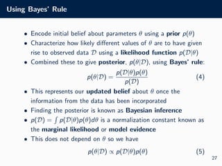
Supervised Learning
7
Datapoint
Index
x1 x2 x3 … xM
1 0.24 0.12 -0.34 … 0.98
2 0.56 1.22 0.20 … 1.03
3 -3.20 -0.01 0.21 … 0.93
… … … … … …
N 2.24 1.76 -0.47 … 1.16
y
3
2
1
…
2
Training
Data Input Features
}
}
Outputs
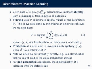
• Use this data to learn a predictive model fθ : X → Y (e.g. by
optimizing θ)
• Once learned, we can use this to predict outputs for new input
points, e.g. fθ([0.48 1.18 0.34 . . . 1.13]) = 2
13

16. Unsupervised Learning
• In unsupervised Learning we have no clear output variable
that we are attempting to predict: D = {xn}N
n=1
• This is sometimes referred to as unlabeled data
• Aim is to exact some salient features for the dataset, such as
underlying structure, patterns, or characteristics
• Examples: clustering, feature extraction, density estimation,
representation learning, data visualization, data compression
14

17. Unsupervised Learning—Clustering
Classification
Cat
Unlabeled Data Group into Clusters
15

18. Unsupervised Learning—Deep Generative Models
Learn powerful models for generating new datapoints
Two major unsolved problems in the field of machine learning are (1) data-efficiency: the ability to
learn from few datapoints, like humans; and (2) generalization: robustness to changes of the task or
its context. AI systems, for example, often do not work at all when given inputs that are different
⇤
Equal contribution.
32nd Conference on Neural Information Processing Systems (NeurIPS 2018), Montréal, Canada.
Figure 1: Synthetic celebrities sampled from our model; see Section 3 for architecture and method,
and Section 5 for more results.
These are not real faces: they are samples from a learned model!
1
D P Kingma and P Dhariwal. “Glow: Generative flow with invertible 1x1 convolutions”. In: NeurIPS. 2018. 16

19. Discriminative vs
Generative Machine
Learning
16

20. Discriminative vs Generative Machine Learning
• Discriminative methods try to directly predict outputs (they
are primary used for supervised tasks)
• Generative methods try to explain how the data was
generated
Image credit: Jason Martuscello, medium.com
17

21. Discriminative Machine Learning
• Given data D = {xn, yn}N
n=1, discriminative methods directly
learn a mapping fθ from inputs x to outputs y
• Training uses D to estimate optimal values of the parameters
θ∗. This is typically done by minimizing an empirical risk over
the training data:
θ∗
= arg min
θ
1
N
N
X
n=1
L(yi , fθ(xi )) (1)
where L(y, ŷ) is a loss function for prediction ŷ and truth y.
• Prediction at a new input x involves simply applying fθ̂(x),
where θ̂ is our estimate of θ∗
• Note we often do not predict y directly, e.g. in a classification
task we might predict the class probabilities instead
• For non-parametric approaches, the dimensionality of θ
increases with the dataset size 18

22. Discriminative Machine Learning
Common approaches: neural networks, support vector machines,
random forests, linear/logistic regression
Pros
• Simpler to directly solve prediction problem than model the
whole data generation process
• Few assumptions
• Often very effective for large datasets
• Some methods can be used effectively in a black-box manner
Cons
• Can be difficult to impart prior information
• Typically lack interpretability
• Do not usually provide natural uncertainty estimates
19

23. Generative Machine Learning
• Generative approaches construct a probabilistic model to
explain how the data is generated
• For example, with labeled data D = {xn, yn}N
n=1, we might
construct a model p(x, y; θ) of the form xn ∼ p(x; θ),
yn|xn ∼ p(y|x = xn; θ) where θ are model parameters
• This in turns implies a predictive model
• Can also be generative about the model parameters θ:
e.g. with unsupervised data D = {xn}N
n=1, we can construct a
generative model p(θ, x), such that θ ∼ p(θ), xn|θ ∼ p(x|θ).
• This is the foundation for Bayesian machine learning
20

24. Generative Machine Learning
Common approaches: Bayesian approaches, deep generative
models, mixture models
Pros
• Allow us to make stronger modeling assumptions and thus
incorporate more problem–specific expertise
• Provide explanation for how data was generated
• More interpretable
• Can provide additional information other than just prediction
• Many methods naturally provide uncertainty estimates
• Allow us to use Bayesian methods
21

25. Generative Machine Learning
Cons
• Can be difficult to construct—typically require problem
specific expertise
• Can impart unwanted assumptions—often less effective for
huge datasets
• Tackling an inherently more difficult problem than straight
prediction
22

26. The Bayesian Paradigm
22

27. Bayesian Probability is All About Belief
Frequentist Probability
The frequentist interpretation of probability is that it is the average
proportion of the time an event will occur if a trial is repeated
infinitely many times.
Bayesian Probability
The Bayesian interpretation of probability is that it is the
subjective belief that an event will occur in the presence of
incomplete information
23

28. Bayesianism vs Frequentism
https://xkcd.com/1132/ 24

29. Bayesianism vs Frequentism
https://xkcd.com/1132/
24

30. Bayesianism vs Frequentism
https://xkcd.com/1132/
24

31. Bayesianism vs Frequentism
Warning
Bayesiansism has its shortfalls too—see the course notes
24

32. The Basic Laws of Probability
We can derive most of Bayesian statistics from two rules:
The Product Rule
The probability of two events occurring is the probability of one of
the events occurring times the conditional probability of the other
event happening given the first event happened:
P(A, B) = P(A|B)P(B) = P(B|A)P(A) (2)
The Sum Rule
The probability that either A or B occurs, P(A ∪ B), is given by
P(A ∪ B) = P(A) + P(B) − P(A, B). (3)
25

33. Bayes’ Rule
p(B|A) =
p(A|B)p(B)
p(A)
26

34. Using Bayes’ Rule
• Encode initial belief about parameters θ using a prior p(θ)
• Characterize how likely different values of θ are to have given
rise to observed data D using a likelihood function p(D|θ)
• Combined these to give posterior, p(θ|D), using Bayes’ rule:
p(θ|D) =
p(D|θ)p(θ)
p(D)
(4)
• This represents our updated belief about θ once the
information from the data has been incorporated
• Finding the posterior is known as Bayesian inference
• p(D) =
R
p(D|θ)p(θ)dθ is a normalization constant known as
the marginal likelihood or model evidence
• This does not depend on θ so we have
p(θ|D) ∝ p(D|θ)p(θ) (5)
27

35. Multiple Observations: Using the Posterior as the Prior
• One of the key characteristics of Bayes’ rule is that it is
self-similar under multiple observations
• We can use the posterior after our first observation as the
prior when considering the next:
p(θ|D1, D2) =
p(D2|θ, D1)p(θ|D1)
p(D2|D1)
(6)
=
p(D2|θ, D1)p(D1|θ)p(θ)
p(D2|D1)p(D1)
(7)
=
p(D1, D2|θ)p(θ)
p(D1, D2)
(8)
• We can thinking of this as continuous updating of beliefs as
we receive more information
28

36. Example: Positive Cancer Test
We have just had a result back from the Doctor for a cancer
screen and it comes back positive. How worried should we be given
the test isn’t perfect?
29

37. Example: Positive Cancer Test (2)
Before these results came in, the chance of us having this type of
cancer was quite low: 1/1000. Let’s say θ represents us having
cancer so our prior is p(θ) = 1/1000.
For people who do have cancer, the test is 99.9% accurate.
Denoting the event of the test returning positive as D = 1, we
thus have p(D = 1|θ = 1) = 999/1000.
For people who do not have cancer, the test is 99% accurate. We
thus have p(D = 1|θ = 0) = 1/100.
Our prospects might seem quite grim at this point given how
accurate the test is.
30

38. Example: Positive Cancer Test (3)
To figure out the chance we have cancer properly though, we now
need to apply Bayes rule:
p(θ = 1|D = 1) =
p(D = 1|θ = 1)p(θ = 1)
p(D = 1)
=
p(D = 1|θ = 1)p(θ = 1)
p(D = 1|θ = 1)p(θ = 1) + p(D = 1|θ = 0)p(θ = 0)
=
0.999 × 0.001
0.999 × 0.001 + 0.01 × 0.999
= 1/11
So the chances are that we actually don’t have cancer!
31

39. Alternative Viewpoint
An alternative (equivalent) viewpoint for Bayesian reasoning is that
we first define a joint model over parameters and data: p(θ, D)
We then condition this model on the data taking the observed
value, i.e. we fix D
This produces the posterior p(θ|D) by simply normalizing this to
be a valid probability distribution, i.e. the posterior is proportional
to the joint for a fixed D:
p(θ|D) ∝ p(θ, D) (9)
32

40. How Might we Write a System to Break Captchas?
Bridging the Gap Between the Bayesian Ideal and Common Practice
Tom Rainforth
2 3 4
x2 = ≠1 x3 = 6 x4
⁄” a6 = “⁄” a7 = “⁄” a8
i6 = 4 i7 = 5 i8
8 x6 = 53 x7 = 17 x8
⁄” Noise: Noise: No
displacement stroke ell
field
e 6: Pseudo algorithm and a sample
2
33

41. Simulating Captchas is Much Easier
Bridging the Gap Between the Bayesian Ideal and Common Practice
Tom Rainforth
[Le, Baydin, and Wood. Inference Compilation and Universal
Inference
Generation
a5 = “⁄” a6 = “⁄
i5 = 3 i6 = 4
x5 = 18 x6 = 53
a9 = “⁄” Noise:
i9 = 7 displace
x9 = 9 field
i2 = 1 i3 = 1
x2 = ≠1 x3 = 6
” a6 = “⁄” a7 = “⁄
i6 = 4 i7 = 5
8 x6 = 53 x7 = 17
” Noise: Noise:
displacement stroke 3
gxs2rRj
34

42. The Bayesian Pipeline
Bridging the Gap Between the Bayesian Ideal and Common Practice
Tom Rainforth
The Bayesian Pipeline
Inference
Method
}
Prior
p(✓)
}
Likelihood
p(D|✓)
Data
}
D
Posterior
}
p(✓|D) / p(D|✓)p(✓)
35

43. Breaking Captchas with Bayesian Models
https://youtu.be/ZTKx4TaqNrQ?t=9
2
TA Le, A G Baydin, and F Wood. “Inference Compilation and Universal Probabilistic Programming”. In:
AISTATS. 2017.
36

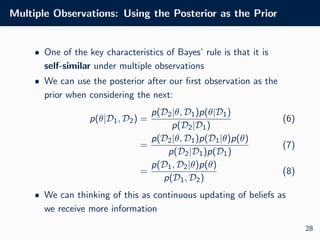
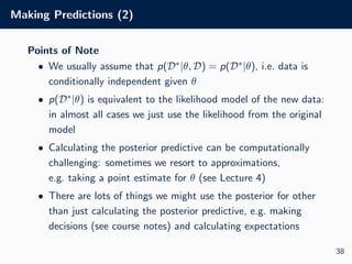
44. Making Predictions
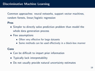
• Prediction in Bayesian models is done using the posterior
predictive distribution
• This is defined by taking the expectation of a predictive model
for new data, p(D∗|θ, D), with respect to the posterior:
p(D∗
|D) =
Z
p(D∗
, θ|D)dθ (10)
=
Z
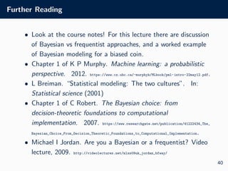
p(D∗
|θ, D)p(θ|D)dθ (11)
= Ep(θ|D)[p(D∗
|θ, D)]. (12)
• This often done dependent on an input point, i.e. we actually
calculate p(y|D, x) = Ep(θ|D)[p(y|θ, D, x)]
37

45. Making Predictions (2)
Points of Note
• We usually assume that p(D∗|θ, D) = p(D∗|θ), i.e. data is
conditionally independent given θ
• p(D∗|θ) is equivalent to the likelihood model of the new data:
in almost all cases we just use the likelihood from the original
model
• Calculating the posterior predictive can be computationally
challenging: sometimes we resort to approximations,
e.g. taking a point estimate for θ (see Lecture 4)
• There are lots of things we might use the posterior for other
than just calculating the posterior predictive, e.g. making
decisions (see course notes) and calculating expectations
38

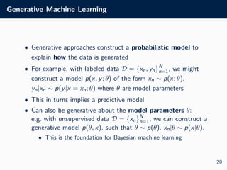
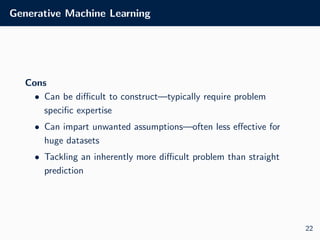
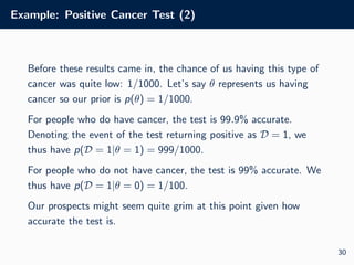
46. Recap
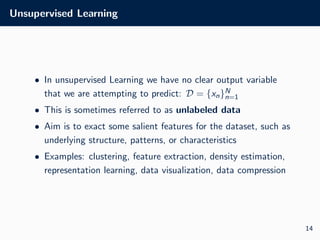
• Supervised learning has access to outputs, unsupervised
learning does not
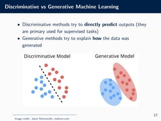
• Discriminative methods try and directly make predictions,
generative methods try to explain how the data is generated
• Bayesian machine learning is a generative approach that
allows us to incorporate uncertainty and information from
prior expertise
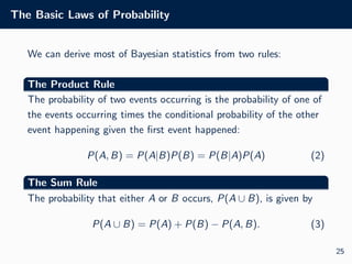
• Bayes’ rule: p(θ|D) ∝ p(D|θ)p(θ)
• Posterior predictive: p(D∗|D) = Ep(θ|D) [p(D∗|θ, D)]
39

47. Further Reading
• Look at the course notes! For this lecture there are discussion
of Bayesian vs frequentist approaches, and a worked example
of Bayesian modeling for a biased coin.
• Chapter 1 of K P Murphy. Machine learning: a probabilistic
perspective. 2012. https://www.cs.ubc.ca/~murphyk/MLbook/pml-intro-22may12.pdf.
• L Breiman. “Statistical modeling: The two cultures”. In:
Statistical science (2001)
• Chapter 1 of C Robert. The Bayesian choice: from
decision-theoretic foundations to computational
implementation. 2007. https://www.researchgate.net/publication/41222434_The_
Bayesian_Choice_From_Decision_Theoretic_Foundations_to_Computational_Implementation.
• Michael I Jordan. Are you a Bayesian or a frequentist? Video
lecture, 2009. http://videolectures.net/mlss09uk_jordan_bfway/
40