Downloaded 132 times
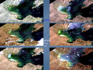
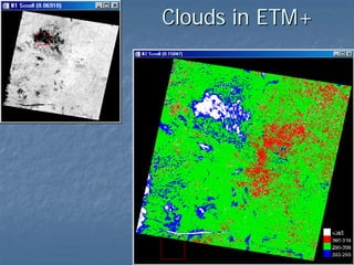
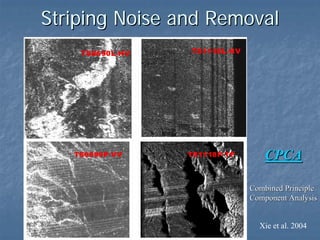
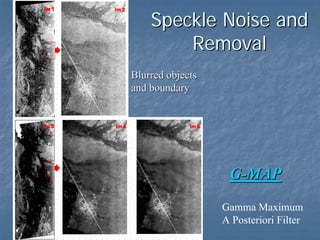
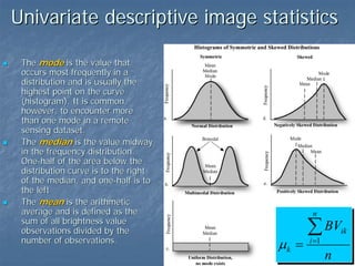
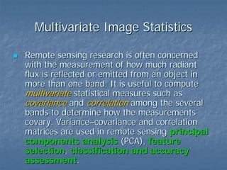
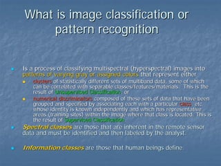
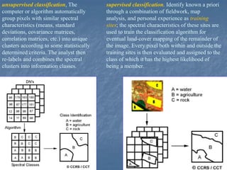
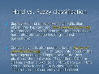
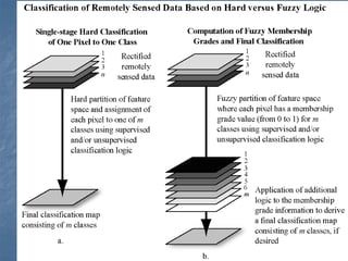
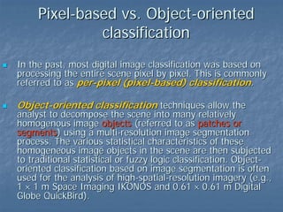

This document provides an overview of digital image processing. It discusses what image processing entails, including enhancing images, extracting information, and pattern recognition. It also describes various image processing techniques such as radiometric and geometric correction, image enhancement, classification, and accuracy assessment. Radiometric correction aims to reduce noise from sources like the atmosphere, sensors, and terrain. Geometric correction geometrically registers images. Image enhancement improves interpretability. Classification categorizes pixels. The document outlines both supervised and unsupervised classification methods.