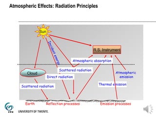
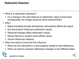
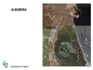
ATMOSPHERIC INFLUENCE ON IMAGES AND
THE CORRECTION.
GABRIEL PARODI
Sun
R.S. Instrument
Scattered
radiation
Cloud
Atmospheric
emission
Emission processesReflection processesEARTH
Atmosperic absortion
Direct
radiation
Reflected
radiation
Thermal
emission
Scattered
radiation
Thermal emission
Atmospheric
emission
R.S. Instrument
Sun
Cloud
Scattered radiation
Direct radiation
Scattered radiation
Atmospheric absorption
Earth Reflection processes Emission processes
Atmospheric Effects: Radiation Principles
Radiometric Distortion
 What is a radiometric distortion?
 It’s a change in the real radiance or radiometric value of pixel (and
consequently, the image) cause by some external factor.
 Why?
 Signal travelling through atmosphere; atmosphere affects the signal
 Sun illumination influences radiometric values
 Seasonal changes affect radiometric values
 Sensor failures or system noise affects values
 Terrain influences radiance
 When we need to correct for this influence
 When we are interested in a land property related to real reflectance
 When we need to compare reflectance changes in two different dates
Line Striping: Landsat TM Example
De-stripedStriping
Line Striping: SPOT XS Example
De-stripedStriping
Line drop outs: Dropped Signal - Example
(CCRS Remote Sensing Tutorial)
Random noise or spikes
 Example of Spikes in Landsat MSS
Haze – Example (Indonesia)
Haze Effect Corrected Image
Remote sensing methods: From ground to satellite
Atmosphere
Surface
Satellite
Satellite DN
Calibration
Atmospheric
correction
Soil information
Direct
problem
Inverse problem
Radiance TOA= ao +a1 *
Dn
Radiance TOA  Real
Radiance
Primary parameters Secondary parameters Tertiary parameters
Solar radiance Reflectivity Solar radiation
Earth radiance Temperature Evapotranspiration
Error= 1 % Error= 10 % Error= 20 %
Inverse problem:
Given TOA get
Surface
Atmospheric correction methods
 Atmospheric correction is the procedure that reduces the effect of
scattering and absorption in the signal
 Two procedures:
 Relative AC methods based on ground reflectance (seen here)
 Absolute AC methods based on atmospheric processes they
will be seen later
Two reference surfaces (1)
Master date A Slave date B
ρMB
ρMD
ρSD
ρSB
 Input: 1 band of a satellite in date A (called master) and the same band in a date B (slave)
 Output is not and atmospherically corrected image BUT an image matching a reflectance compatible with
the atmosphere of another similar image taken a previous date, allows comparative results only.
 It does not requires field measurements but reflective invariant areas (areas that do not change
reflectance in time)
 Find reflectance invariants in both images (sand, water, forest, quarry, etc) and relate them linearly
Two reference surfaces: Analysis
 If the atmosphere would be the same in the two dates, then the reflectance of the invariants by
definition should be identical.
 Since the atmosphere is not the same, there is a difference in reflectance of the invariants
 Plotting the difference in reflectance vs. the reflectance of the slave image (only for the
invariants), then a linear relation is found.
 The procedure ends by calculating a new “artificial” slave image having a ground reflectance that
would be the one of the slave image if that day the atmosphere would be the same as the atmosphere
of the master image.
 Now the master and the slave image can be compared since the atmosphere was forced to be the
same in both images. So, if there are cahnges in the reflectances it will not be due to the atmosphere.
SDMDandSBMB  
SDMDDandSBMBB  
linearSF )( 
functionlinearMF )( 
S
B
D
 SS'
Field and laboratory spectrometry
0
10000
20000
30000
40000
50000
60000
70000
250 500 750 1000 1250 1500 1750 2000 2250 2500
Target Reference
-50000
0
50000
100000
150000
200000
250000
300000
350000
400000
250 500 750 1000 1250 1500 1750 2000 2250 2500
Target Reference
Two Reflectance Measurements
 Input: one band of a satellite to be atmospherically corrected
 Output is the atmospherically corrected image band, so, it allows flux quantification
 Requires radiometric field measurements at bright and dark targets in identical
wavelength range
TOA radiance Sat= RSatbright
Radiance at ground: RGbright
TOA radiance Sat= RSatdark
Radiance at ground: RGground
Radiance Ground
Radiance TOA
Ground Corr= a + TOA * b
ALBUFERA OF VALENCIA: STUDY CASE
GABRIEL PARODI
ALBUBERA
SAMPLES TABLE
Sample nr Time X Y Index A Index B Index C
1 11:27 726127.348 4355474.044 28 420 68
2 9:10 727040.823 4354865.060 25 660 69
3 10:10 727606.308 4355256.550 21 462 56
4 9:40 727632.407 4355839.434 14 341 55
5 9:00 727588.908 4356518.016 20 341 54
6 9:30 727388.813 4357300.994 17 173 43
7 10:50 727171.319 4358127.472 20 285 58
8 9:55 726797.229 4358919.151 19 442 52
9 8:45 729763.849 4356056.928 15 415 61
10 9:00 729781.249 4356378.819 9 487 60
11 9:20 729850.847 4356874.706 14 417 60
12 9:40 729720.350 4357466.290 9 352 55
13 9:50 729589.854 4357962.176 14 287 46
14 9:15 729563.755 4358553.760 18 268 54
15 9:30 729589.854 4359223.642 22 539 68
16 10:00 729485.457 4359641.231 18 601 67
17 10:10 728658.979 4357683.784 20 135 56
18 10:22 730590.327 4358727.756 16 123 37
19 10:40 730529.428 4359093.146 18 201 53
20 11:05 730416.332 4359615.132 13 305 45
SAMPLES DISTRIBUTION
REFLECTANCE AND CONTAMINANTS
Figure 1: Best relation for Index_A in
red. Error shows in black dotted lines.
Figure 2: Best relation for Index_B.
Error shows in black dotted lines.
Figure 3: Best relation for Index_C. Error
shows in black dotted lines.
Atmospheric correction albufera_web

Atmospheric correction albufera_web

  • 1.
    ATMOSPHERIC INFLUENCE ONIMAGES AND THE CORRECTION. GABRIEL PARODI
  • 2.
    Sun R.S. Instrument Scattered radiation Cloud Atmospheric emission Emission processesReflectionprocessesEARTH Atmosperic absortion Direct radiation Reflected radiation Thermal emission Scattered radiation Thermal emission Atmospheric emission R.S. Instrument Sun Cloud Scattered radiation Direct radiation Scattered radiation Atmospheric absorption Earth Reflection processes Emission processes Atmospheric Effects: Radiation Principles
  • 3.
    Radiometric Distortion  Whatis a radiometric distortion?  It’s a change in the real radiance or radiometric value of pixel (and consequently, the image) cause by some external factor.  Why?  Signal travelling through atmosphere; atmosphere affects the signal  Sun illumination influences radiometric values  Seasonal changes affect radiometric values  Sensor failures or system noise affects values  Terrain influences radiance  When we need to correct for this influence  When we are interested in a land property related to real reflectance  When we need to compare reflectance changes in two different dates
  • 4.
    Line Striping: LandsatTM Example De-stripedStriping
  • 5.
    Line Striping: SPOTXS Example De-stripedStriping
  • 6.
    Line drop outs:Dropped Signal - Example (CCRS Remote Sensing Tutorial)
  • 7.
    Random noise orspikes  Example of Spikes in Landsat MSS
  • 8.
    Haze – Example(Indonesia) Haze Effect Corrected Image
  • 9.
    Remote sensing methods:From ground to satellite Atmosphere Surface Satellite Satellite DN Calibration Atmospheric correction Soil information Direct problem Inverse problem Radiance TOA= ao +a1 * Dn Radiance TOA  Real Radiance Primary parameters Secondary parameters Tertiary parameters Solar radiance Reflectivity Solar radiation Earth radiance Temperature Evapotranspiration Error= 1 % Error= 10 % Error= 20 % Inverse problem: Given TOA get Surface
  • 10.
    Atmospheric correction methods Atmospheric correction is the procedure that reduces the effect of scattering and absorption in the signal  Two procedures:  Relative AC methods based on ground reflectance (seen here)  Absolute AC methods based on atmospheric processes they will be seen later
  • 11.
    Two reference surfaces(1) Master date A Slave date B ρMB ρMD ρSD ρSB  Input: 1 band of a satellite in date A (called master) and the same band in a date B (slave)  Output is not and atmospherically corrected image BUT an image matching a reflectance compatible with the atmosphere of another similar image taken a previous date, allows comparative results only.  It does not requires field measurements but reflective invariant areas (areas that do not change reflectance in time)  Find reflectance invariants in both images (sand, water, forest, quarry, etc) and relate them linearly
  • 12.
    Two reference surfaces:Analysis  If the atmosphere would be the same in the two dates, then the reflectance of the invariants by definition should be identical.  Since the atmosphere is not the same, there is a difference in reflectance of the invariants  Plotting the difference in reflectance vs. the reflectance of the slave image (only for the invariants), then a linear relation is found.  The procedure ends by calculating a new “artificial” slave image having a ground reflectance that would be the one of the slave image if that day the atmosphere would be the same as the atmosphere of the master image.  Now the master and the slave image can be compared since the atmosphere was forced to be the same in both images. So, if there are cahnges in the reflectances it will not be due to the atmosphere. SDMDandSBMB   SDMDDandSBMBB   linearSF )(  functionlinearMF )(  S B D  SS'
  • 13.
    Field and laboratoryspectrometry 0 10000 20000 30000 40000 50000 60000 70000 250 500 750 1000 1250 1500 1750 2000 2250 2500 Target Reference -50000 0 50000 100000 150000 200000 250000 300000 350000 400000 250 500 750 1000 1250 1500 1750 2000 2250 2500 Target Reference
  • 14.
    Two Reflectance Measurements Input: one band of a satellite to be atmospherically corrected  Output is the atmospherically corrected image band, so, it allows flux quantification  Requires radiometric field measurements at bright and dark targets in identical wavelength range TOA radiance Sat= RSatbright Radiance at ground: RGbright TOA radiance Sat= RSatdark Radiance at ground: RGground Radiance Ground Radiance TOA Ground Corr= a + TOA * b
  • 15.
    ALBUFERA OF VALENCIA:STUDY CASE GABRIEL PARODI
  • 16.
  • 17.
    SAMPLES TABLE Sample nrTime X Y Index A Index B Index C 1 11:27 726127.348 4355474.044 28 420 68 2 9:10 727040.823 4354865.060 25 660 69 3 10:10 727606.308 4355256.550 21 462 56 4 9:40 727632.407 4355839.434 14 341 55 5 9:00 727588.908 4356518.016 20 341 54 6 9:30 727388.813 4357300.994 17 173 43 7 10:50 727171.319 4358127.472 20 285 58 8 9:55 726797.229 4358919.151 19 442 52 9 8:45 729763.849 4356056.928 15 415 61 10 9:00 729781.249 4356378.819 9 487 60 11 9:20 729850.847 4356874.706 14 417 60 12 9:40 729720.350 4357466.290 9 352 55 13 9:50 729589.854 4357962.176 14 287 46 14 9:15 729563.755 4358553.760 18 268 54 15 9:30 729589.854 4359223.642 22 539 68 16 10:00 729485.457 4359641.231 18 601 67 17 10:10 728658.979 4357683.784 20 135 56 18 10:22 730590.327 4358727.756 16 123 37 19 10:40 730529.428 4359093.146 18 201 53 20 11:05 730416.332 4359615.132 13 305 45
  • 18.
  • 19.
    REFLECTANCE AND CONTAMINANTS Figure1: Best relation for Index_A in red. Error shows in black dotted lines. Figure 2: Best relation for Index_B. Error shows in black dotted lines. Figure 3: Best relation for Index_C. Error shows in black dotted lines.