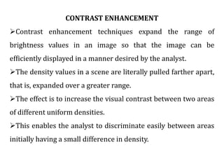
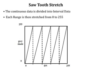
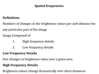
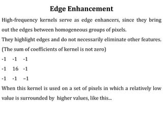
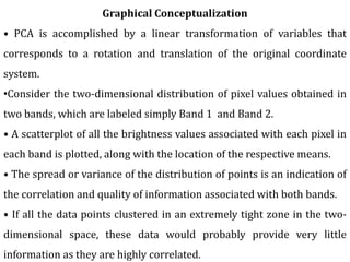
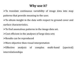
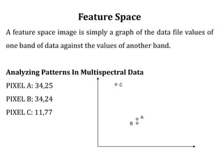
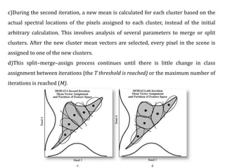
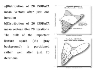
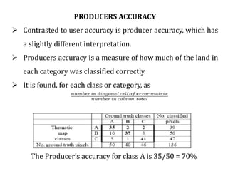
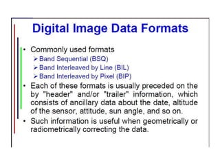
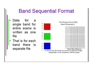
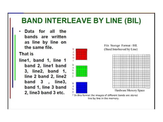
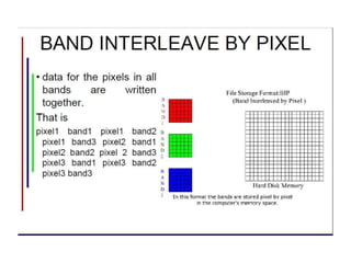
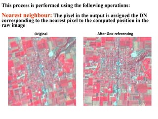
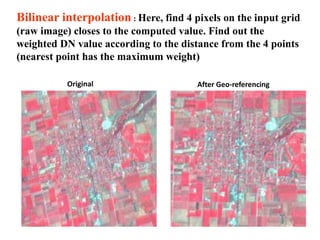
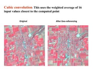
Digital images can be manipulated mathematically by treating pixel brightness values as numbers. This document discusses various digital image processing techniques including:
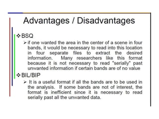
1. Image rectification to correct geometric distortions and calibrate radiometric data. This involves techniques like geometric corrections to adjust for sensor distortions and radiometric corrections to standardize brightness values.
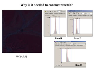
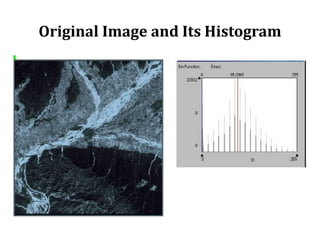
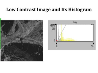
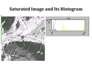
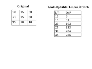
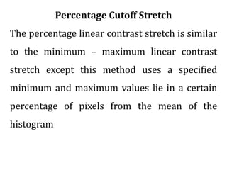
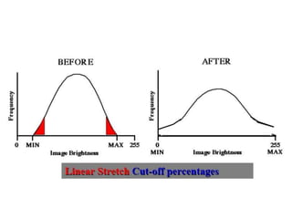
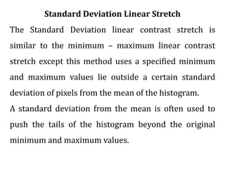
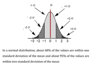
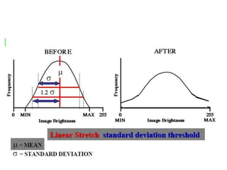
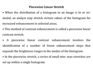
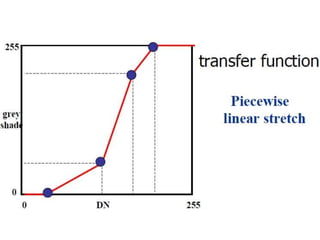
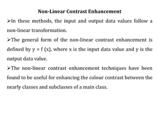
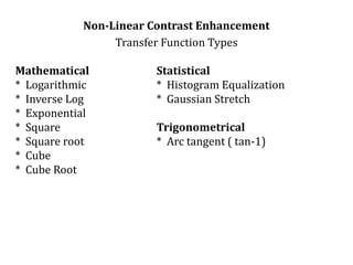
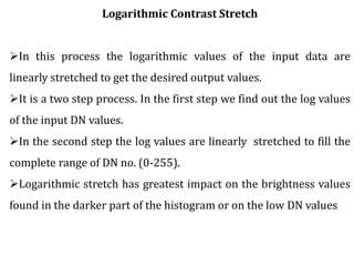
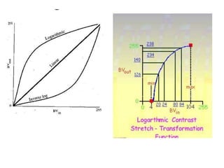
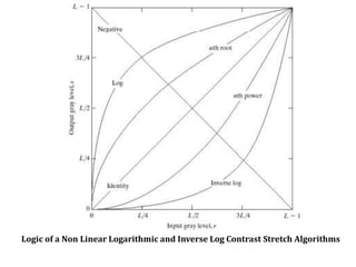
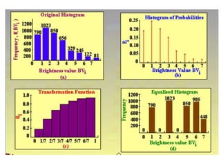
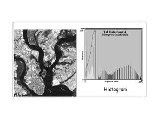
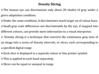
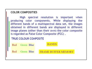
2. Image enhancement techniques like contrast stretching to increase image contrast and improve feature detection. Methods include linear stretches, histogram equalization, and logarithmic transforms.
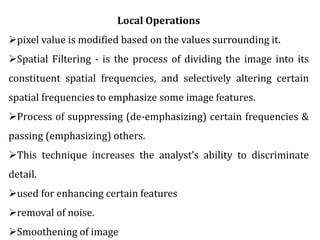
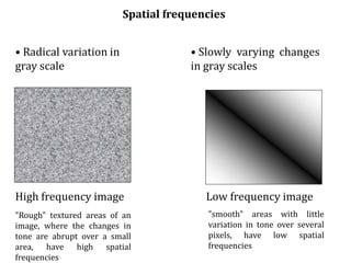
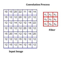
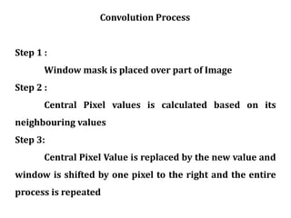
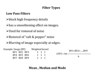
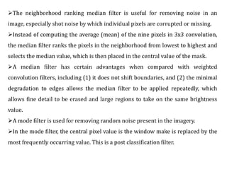
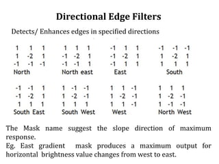
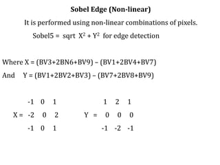
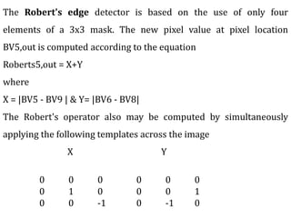
3. Local operations called spatial filtering that modify pixel values based on neighboring pixels. This can emphasize or de-emphasize certain image features or spatial frequencies to enhance details or reduce noise.

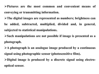
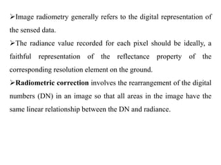
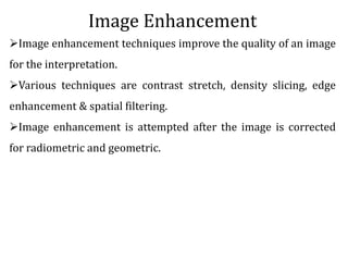
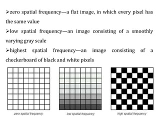
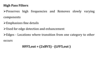
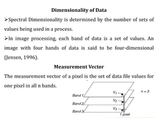
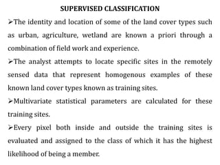
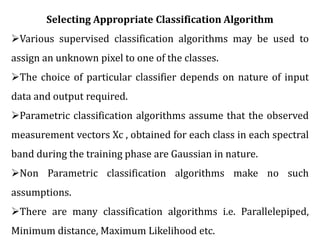
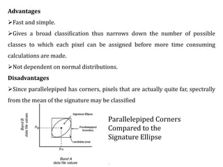
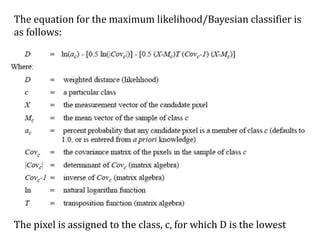
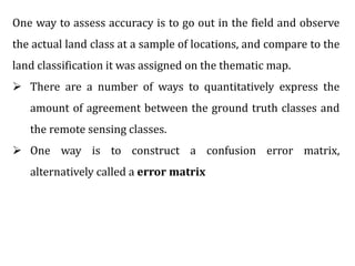
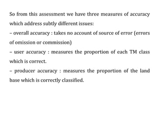
![Part of image with missing scan line
1] Correction for missing lines:
They may be cosmetically corrected in three ways-
a] Replacement by either the preceding or the succeeding line
b] Averaging method
c] Replacement with correlated band](https://image.slidesharecdn.com/digitalimageprocessing-190319054839/85/Digital-image-processing-22-320.jpg)
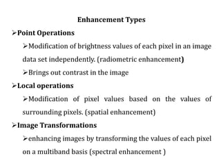
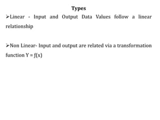
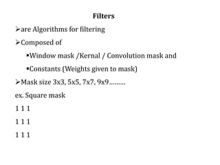
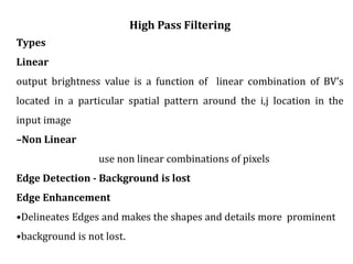
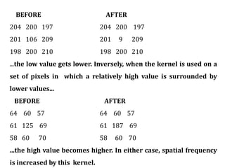
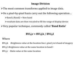
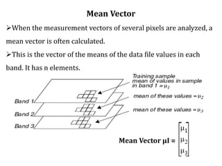
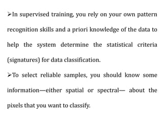
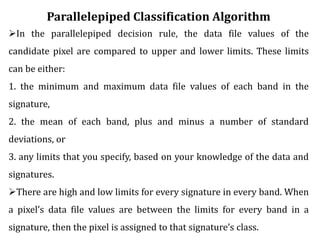
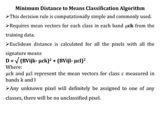
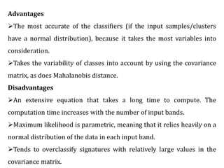
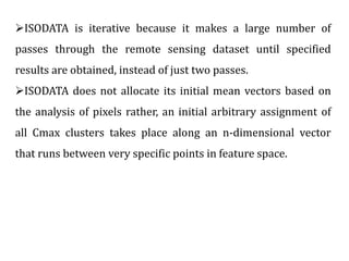
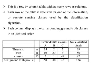
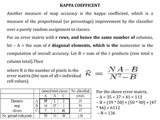
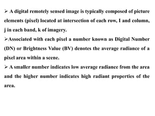
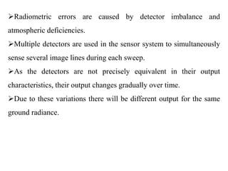
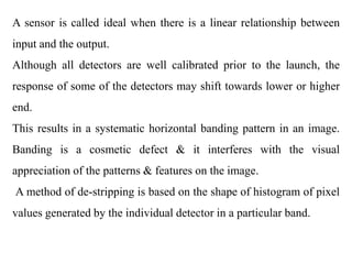
![The Destriped image shows a small improvement compared to the original image
Destriped image (left) Original image (right)
2] Correction for periodic line striping:](https://image.slidesharecdn.com/digitalimageprocessing-190319054839/85/Digital-image-processing-25-320.jpg)
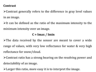
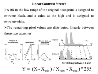
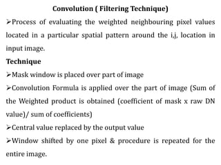
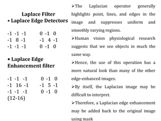
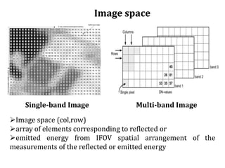
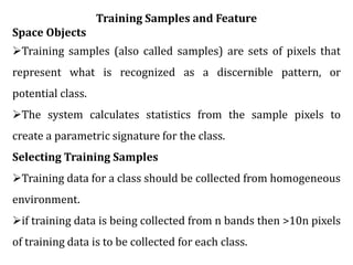
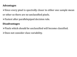
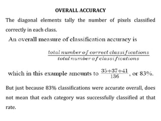
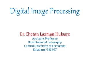
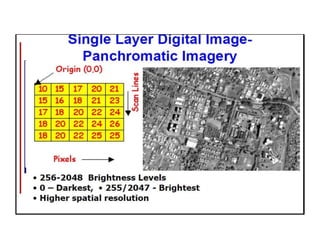
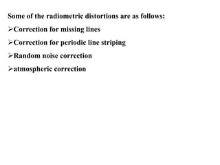
![3] Random noise correction: Random noise means pixels
having offset values from the normal. It can be easily
corrected by means of a smoothing filter on the data](https://image.slidesharecdn.com/digitalimageprocessing-190319054839/85/Digital-image-processing-28-320.jpg)
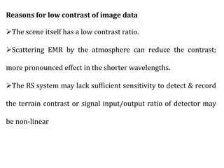
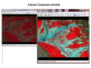
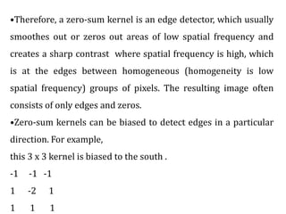
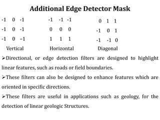
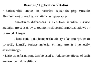
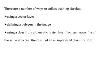
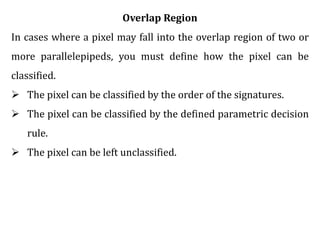
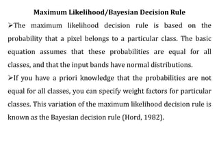
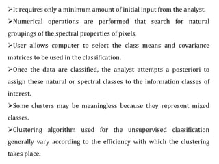
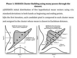
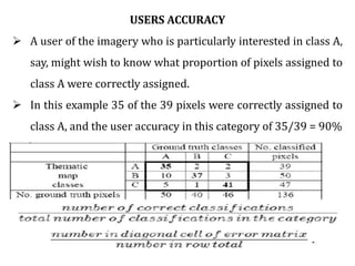
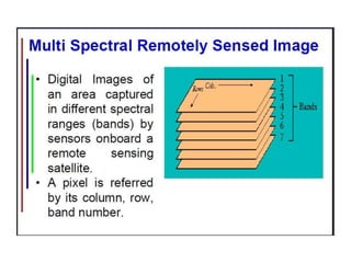
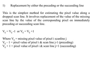
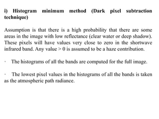
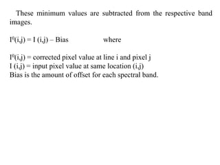
![4] Atmospheric correction: Atmospheric path radiance introduces
haze in the imagery which can be removed by two techniques:
a] Histogram minimum method ( Dark pixel subtraction)
b] Regression method
Atmospheric path luminance correction
Original After correction](https://image.slidesharecdn.com/digitalimageprocessing-190319054839/85/Digital-image-processing-29-320.jpg)
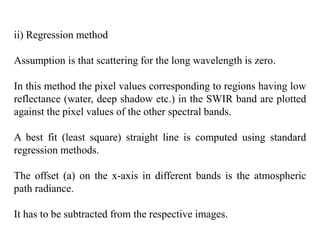
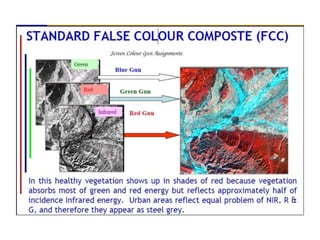
![Geometric Corrections : The geometric correction process is
normally implemented as a 2-step procedure
1] Systematic distortions are well understood and easily
corrected by applying formulas derived by modeling the sources
of the distortions mathematically. They are:
scan skew: Caused by the forward motion of the platform during
the time required for each mirror sweep
mirror-scan velocity: The mirror scanning rate is usually not
constant across a given scan, producing along-scan geometric
distortion](https://image.slidesharecdn.com/digitalimageprocessing-190319054839/85/Digital-image-processing-33-320.jpg)
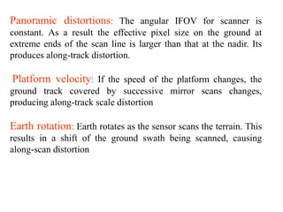
![2] Non systematic distortions
These distortions include errors due to:
1] Platform altitude- If the sensor platform departs from its
normal altitude or the terrain increases in elevation, this produces
changes in scale
2] Attitude- One axis of the sensor system is normal to the Earth's
surface and the other axis is parallel to the spacecraft's direction of
travel
If the sensor departs form this attitude, geometric distortion results
in x, y & z directions which are called roll, pitch & yaw](https://image.slidesharecdn.com/digitalimageprocessing-190319054839/85/Digital-image-processing-35-320.jpg)
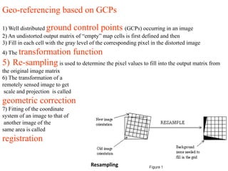
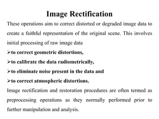
![Application of geometric correction
1] It gives location and scale properties of the desired map
projection to a raw image
2] Registration between images of different bands, of
multiple dates, multiple resolution
3] For mosaicking control points in the overlap region are
used as GCPs](https://image.slidesharecdn.com/digitalimageprocessing-190319054839/85/Digital-image-processing-40-320.jpg)