The document discusses the attitude dynamics of a re-entry vehicle (RV) in planetary atmospheres. It presents the following: 1) Equations of motion for the RV's angular momentum, unit vectors describing its orientation, and acceleration due to aerodynamic and gravitational forces. 2) Equations of motion for the RV's mass center in terms of its velocity, altitude, trajectory inclination angle, and dynamic pressure. 3) Solutions to the undisturbed equations of motion, including an energy integral and general solutions involving elliptic functions for different forms of the restoring aerodynamic moment.

1. Vladimir S. Aslanov
aslanov_vs@mail.ru
Attitude Dynamics of Re-entry Vehicle
Theoretical Mechanics Department
www.termech.ru
Samara State Aerospace University, Russia
www.ssau.ru
2012

2. 1. Statement of the problem
We study of the Re-entry Vehicle (RV) motion about of mass center in the
planetary atmospheres by regular and chaotic dynamics methods
The dynamics of a rotating body studied famous mathematicians of all time as Euler, Poinsot, Lagrange and Kovalevskaya. The
research of the dynamics of rotating bodies is very important for numerous applications such as the dynamics of satellites and re-
entries. In this area we note the papers scientists as Yaroshevsky, Belezky, Rumyantsev, J.Nicolaides, G.Gross, C.Murphy et al.

3. Types of the Re-entry Vehicles.
3

4. 1. Statement of the problem
Aims of research
• To obtain nonlinear mathematical models of the spatial motion of the re-
entry about center of mass in the atmosphere.
• To divide the motion on the unperturbed and perturbed.
• To find to the exact and approximate analytical solutions of the
unperturbed motion.
• To deduce the approximate solutions of the equations of perturbed
motion.
• To determine the nonlinear response and to explore its stability.
• To study the motion of spacecraft in the atmosphere of the methods of
chaotic dynamics.
• To solve the problem of identification of the spacecraft motion over the
small number of the measurements.
4

5. 2. The motion equations
The motion equations of the RV in an inertial frame
   
dK    dei  
2
d r  F
 K  M,    ei  0, 2
g (1)
dt dt dt m
 Coordinate systems

K  I   is angular momentum,

I is inertia tensor,  is angular velocity,
 
F , M are aerodynamic force and moment,

ei is unit vectors,
m is mass of the RV,

g is gravitational acceleration.
5

6. 2. The motion equations
The motion equations of the RV mass center
dV qS d cos   V2  dH
 cxa  g sin  ,   g  ,  V sin  (2)
dt m dt V  r  dt
V 2
V , H,  are velocity, altitude of flight and trajectory q is the dynamic pressure.
inclination angle; 2
Iz  I y
The small asymmetry:   ( yT , zT , i  , I xy , I xz , mx , my , mz )  0( ) (3)
I
where  is a small parameter.
The motion equations about of the RV mass center
d 2
2
 F ( , z )   Ф ( ,  , z ),
dt
d
 R / I x  (G  R cos  ) cos  / sin 2   Ф ( , z ), (4)
dt
dz
  Фz ( ,  , z ), ( z  R, G, q )
dt
F (, z )  (G  R cos )(R  G cos ) / sin3   M  (, z ), (5)
 Ф  D0 ( , z )  D1 ( , z )sin   D ( , z ) cos   D3 ( , z )sin 2  D ( , z) cos 2
 
2

4
(6)
   , R, G, q  6

7. 3. The undisturbed motion
The equations of the undisturbed motion  0
d 2  G  R cos   R  G cos  
  M    0 (7)
dt 2 sin 3 
qSL
The restoring aerodynamic moment M     m   , m    a sin   b sin 2 (8)
I
xT
xT 
L
 *  0,  *  0, *   are the equilibrium position
7

8. 3. The undisturbed motion
Types of the RV
m    a sin   b sin 2
m    a sin 
8

9. 3. The undisturbed motion
Energy integral of equation (7)
1  d  R 2  G 2  2 RG cos 
2
    a cos   b cos 2   E (9)
2  dt  2sin 2
Change of variables u  cos  lead to the equation
2
 du 
   f u  (10)
 dt 
where f  u   2 1  u 2  E  au  bu 2   2GRu  G 2  R 2 (11)
Separating the variables in the equation (10) and integrating it we obtain
u u
du du
t  t0  
u0 f u 
 
u0 a0u  a1u  a2u  a3u  a4
4 3 2 (12)
The integral (12) reduces to the incomplete elliptic integral of the 1st, 2nd and 3rd kind:

d  
d
F ( , k )  

, E ( , k )  1  k sin  d , П ( , n, k )  
2 2
0 1  k 2 sin 2  0 0 (1  n sin 2  ) 1  k 2 sin 2 
9

10. 3. The undisturbed motion
The general solution for m    a sin 
cos   (u1  u2 )cn 2   (t  t0 )  K , k   u2 (13)
где cn   (t  t0 )  K , k   cos am   (t  t0 )  K , k  are elliptic cosine

K  k   F ( , k ) is the complete elliptic integral of 1st kind
2
  am   (t  t0 )  K , k  Is the amplitude-function
The approximate solution
cos   B(1  cos y)(m  cos y)2  u2 (14)
Where y   (t  t0 ) / K , B  (u1  u2 ) p / 8, m  (2  p) / p,
2
 
p  2 1 1 k 2 / 1 1 k 2 
The angle of proper rotation
 R  G  R cos   t   cos  
t
  0    
sin 2   t 

 dt  f П   t  , n1 , k  , П   t  , n2 , k  , П  n1 , k  , П  n2 , k  
0  
 Ix 
(15)
10

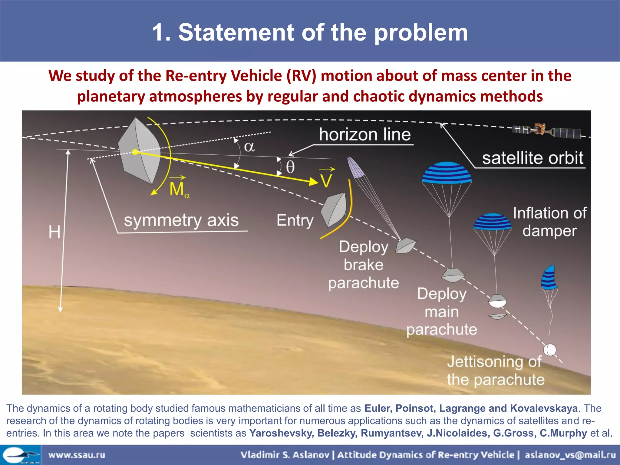
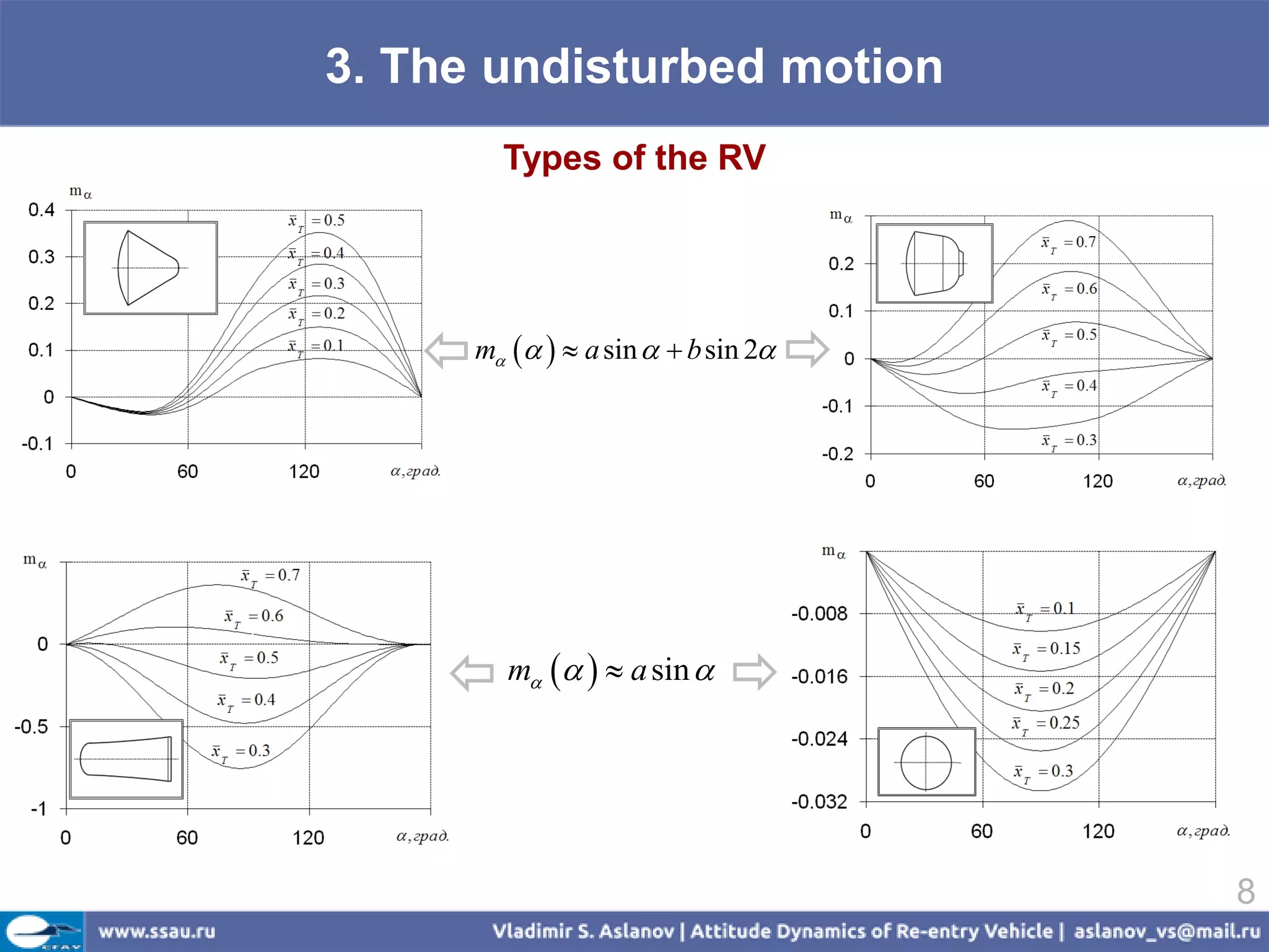
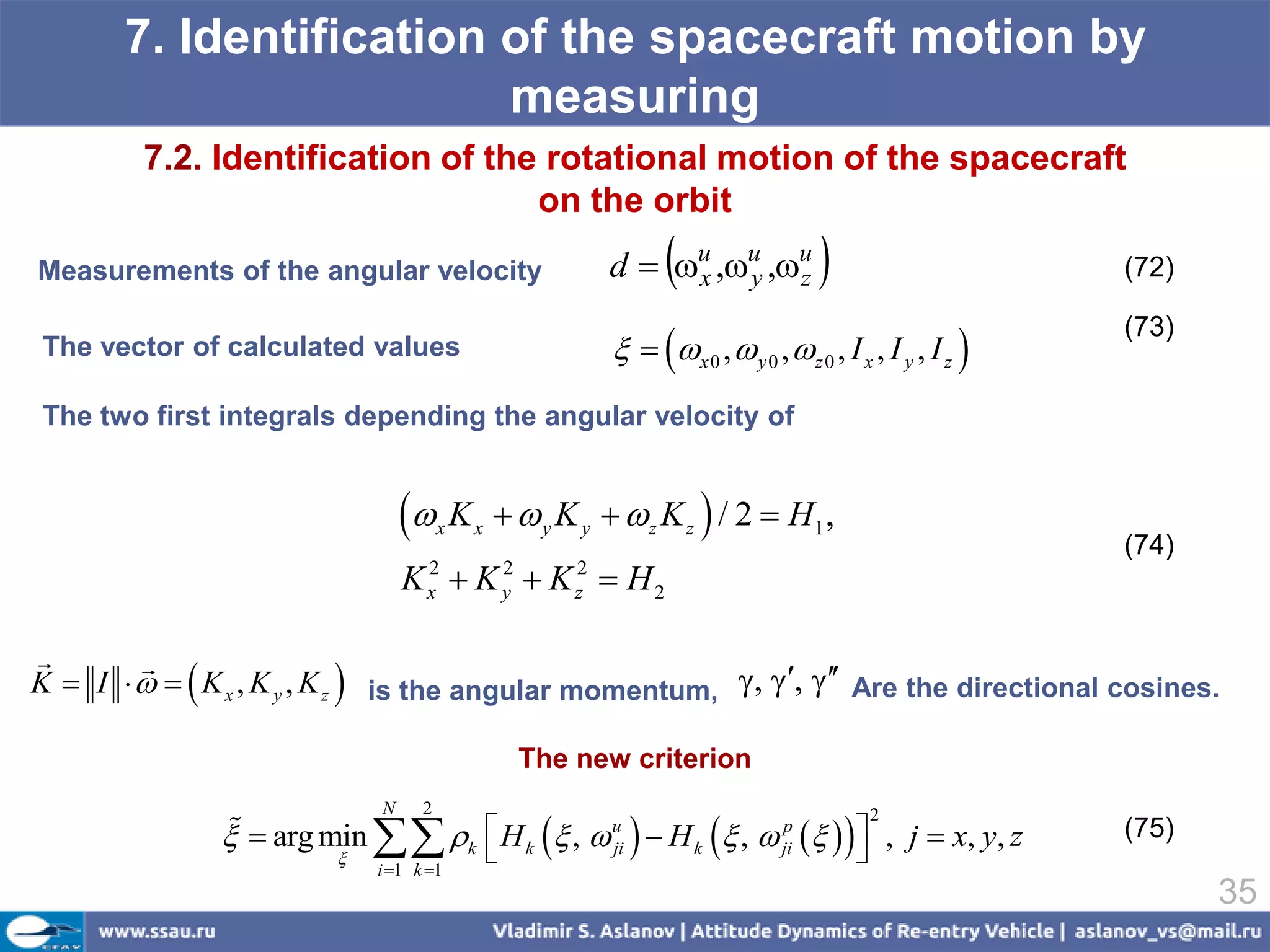
11. 3. The undisturbed motion
The general solution for m    a sin   b sin 2
M
cos   u  L  (16)
1  Ncn 
 t 0, k 
where   1, 2 depends on the type roots of the polynomial: f u   0
The angle of proper rotation
[Vadim Serov]
 R  G  R cos   t   cos  
t
  0    
sin 2   t 

 dt  f ab П   t  , n1 , k  , П   t  , n2 , k  , П  n1 , k  , П  n2 , k  
0  
 Ix 
11

12. 4. The disturbed motion
4.1. The simplest form of the perturbed motion
(asymmetry and damping moments are not available)
Equation of the motion
d 2  G  R cos   R  G cos   dq
  a  q  sin   b  q  sin 2  0,   Фq  t  (17)
dt 2 sin 3  dt
The dependence of the dynamic The dependence of the attack
pressure from time angle from time
12

13. 4. The disturbed motion
The adiabatic invariant is the integral of the perturbed motion
 max
d 1  d 
T 2
Ig 

 dt
d     dt  const
2 0  dt 
(18)
min
Substituting solutions (13) or (16) (18), we obtain an implicit dependence of the
amplitude of the angle of attack of the dynamic pressure
V 2
I g (q  ,  max )  f  K  k  , E (k ), i (k , ni )   const (19)
2
The approximate solutions
 max   max  q  (20)
Minimal angle of attack is determined from the energy integral (9)
 d 
E  0   E  max   E  min  (21)
 dt 
13

14. 4. The disturbed motion
4.2. Perturbed motion of an axisymmetric RV (no asymmetry)
The motion equation
d 2  G  R cos   R  G cos  
  a  q  sin   b  q  sin 2   Ф  , z  ,
dt 2
sin 
3
dz (22)
  Фz ( , z ), ( z  R, G, q)
dt Comparison of the results
where Ф , z  , z   Ф , z   2 , z  
Averaging equations (Volosov method )
d max   1 t T 1
t T
E
F ( max , z )  T  T  z
    dt 
  z dt 
dt
 t t
 W ( max , z ) 
  z     z  , (23)
z 
t T
dz 

dt T t   z ( (t ), z)dt   z  z  ,
where  , z  z    , z  K  k  , E (k ),  i (k , ni ) 
14

15. 4. The disturbed motion
4.3. Disturbed motion of the asymmetric Re-entry Vehicle
The equation of motion in the form of two-frequency system
y  ( z )  Y ( y, , z ),

  Ф ( y, z ),
 (24)
z  Фz ( y, , z ),

Фz  D0z ( y, z)  D1z ( y, z) sin  D2z ( y, z) cos  D3z ( y, z) sin 2  D4z ( y, z) cos 2.
where z  ( R, G ,  max , q ), y  (t  t0 ) is the phase of the attack angle
Фz  y,  , z   Фz  y  2 ,   2 , z  , Ф  y, z   Ф  y  2 , z  ,
(25)
Y  y,  , z   Y  y  2 ,   2 , z 
The average frequency of the proper rotation
2
1
2 
( z )  Ф ( y, z )dy (26)
0
15

16. 4. The disturbed motion
The nonlinear resonance
( z )  m( z )n( z )O() (27)
Where m, n are integer and prime numbers
Approximate formulas for the frequencies(b=0):
 1 1 R2
  2   R / 4,
2
a
2
  R     sign( R  G ) a 
2
(28)
 Ix 2  4
Main resonance (m=n):   (29)
Resonance roll (m=0):  0 (30)
16

17. 4. The disturbed motion
The example of the main resonance(b=0)
qSl  qSl
  F ( )  zт cos  sin 
 , R   zт sin  cos  , q   Фq ( z ), G  const (31)

I I
The main resonance (m=n): 
точка 2
Point 1:
y  0,   0, N1  qS sin  max , M R   z  qSl sin  max N2
N1
N3
Point 2:
точка 1 точка 3
 
y ,  , N 2  qS sin  , M R  0 N4
2 2
Point 3:
y   ,    , N3  qS sin  min , M R  z  qSl sin  min
Point 4: точка 4
3 3
y ,  , N 4  qS sin  , M R  0
2 2
17

18. 4. The disturbed motion
The pendulum system. Analysis of the resonances
Change of the variable:  = my / n   (32) The phase portrait
The pendulum system
d 2 dz
+Q( ,z)=0,   f z (  ,z) (33)
d 2
d
Where    ,
Q(  , z )  Q0 ( z )  Q1 ( z )sin  
(34)
 Q2 ( z ) cos   Q3 ( z )sin 2   Q4 ( z ) cos 2 
The integral of energy    0
2
1  d 
   W ()  E (35)
2  d 
Where W ( ,z)  Q0   Q1 cos   Q2 sin   (36)
1 1
 Q3 cos 2   Q4 sin 2  .
2 2 18

19. 4. The disturbed motion
The capture and pass through the resonance
The main resonance and the resonance roll Types of the motions
 рад.
 проход
захват
 min *  max

t,сек движение в малой
0 50 100 150 200 окрестности центра
19

20. 4. The disturbed motion
The stability of the resonance
Substitution of variables    *   ,    *   ,    d  / d ,  *  0  (37)
The motion equations in the vicinity of the center:   *
d  d 
    G (  * , z ),   2 (  * , z )   P(  * , z ),
d d
(38)
dz
  f z ( * , z)
d
Q Q Q (39)
G( * , z)    f z (  * , z ),  2 (  * , z )  0
 z      *
Wherе /
      *
The Lyapunov function
VA 2
   
2 2
2

20

21. 4. The disturbed motion
The influence of the nonlinear resonance on the RV motion
  гр ад
150
устойчивы й резонанс
125
неустойчивы й резонанс
100
75
50
проход
25
безрезонансное движ ение
h,км
0
65 45 25 5
 к  /с
11 безрезонансное движ ение
проход
10
9
8
7
6
неустойчивы й резонанс
5
4 устойчивы й резонанс h,км
65 45 25 5
21

22. 4. The disturbed motion
4.4. Features of the disturbed motion of the Re-entry Vehicle with the biharmonic moment
The biharmonic moment The phase portrait
m  , t   a  t  sin   b  t  sin 2
The three the equilibrium position:
 *  0,  *  0, *  
Three the areas exist if W   u*1   W   u*2   0 (40)
u*1 , u*2 are roots of the equation W   u   0 (41)
22

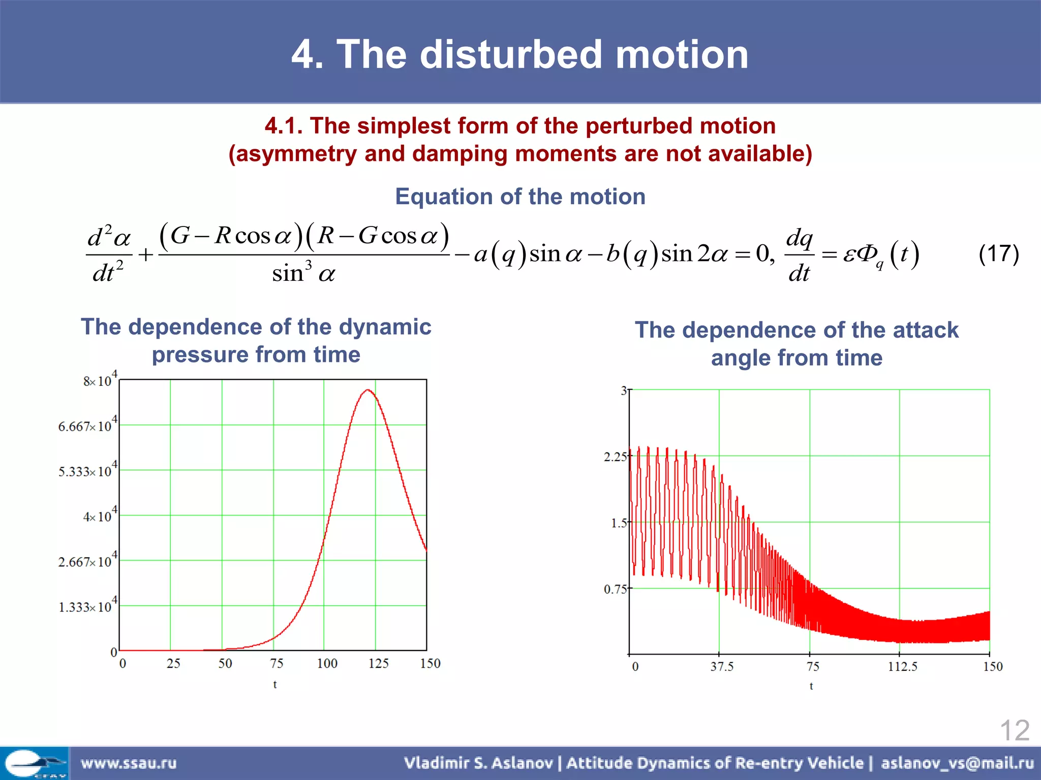
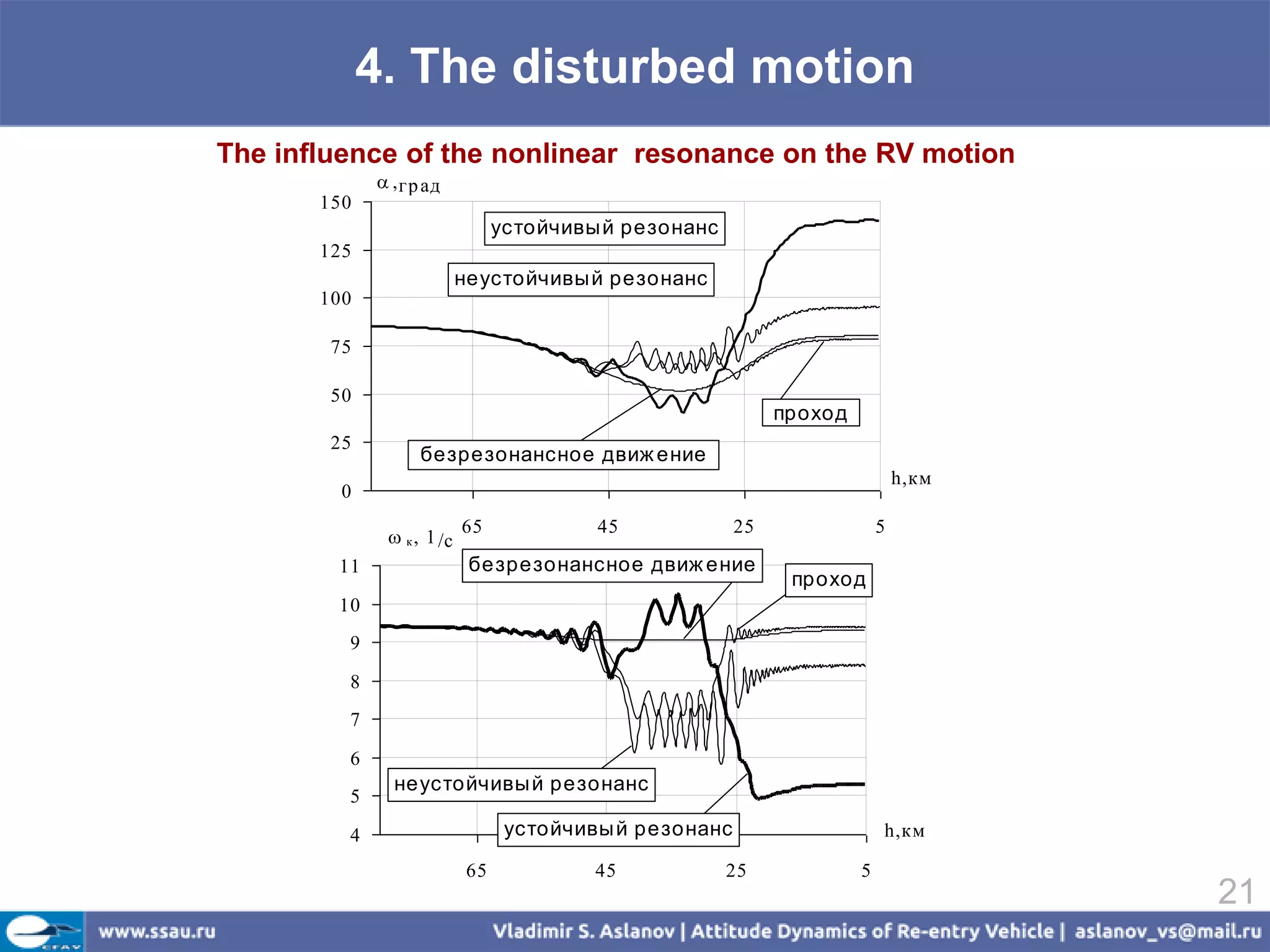
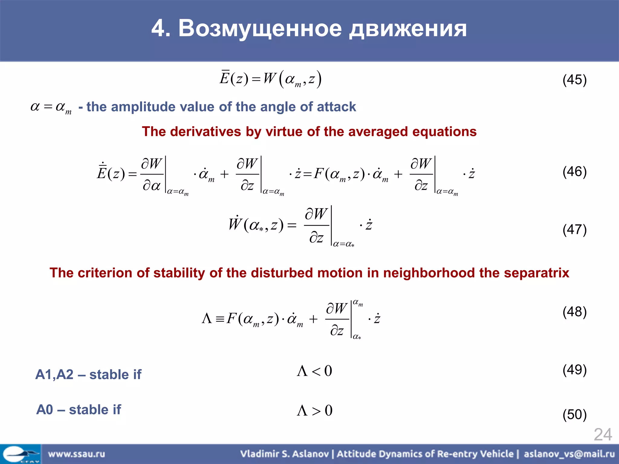
23. 4. The disturbed motion
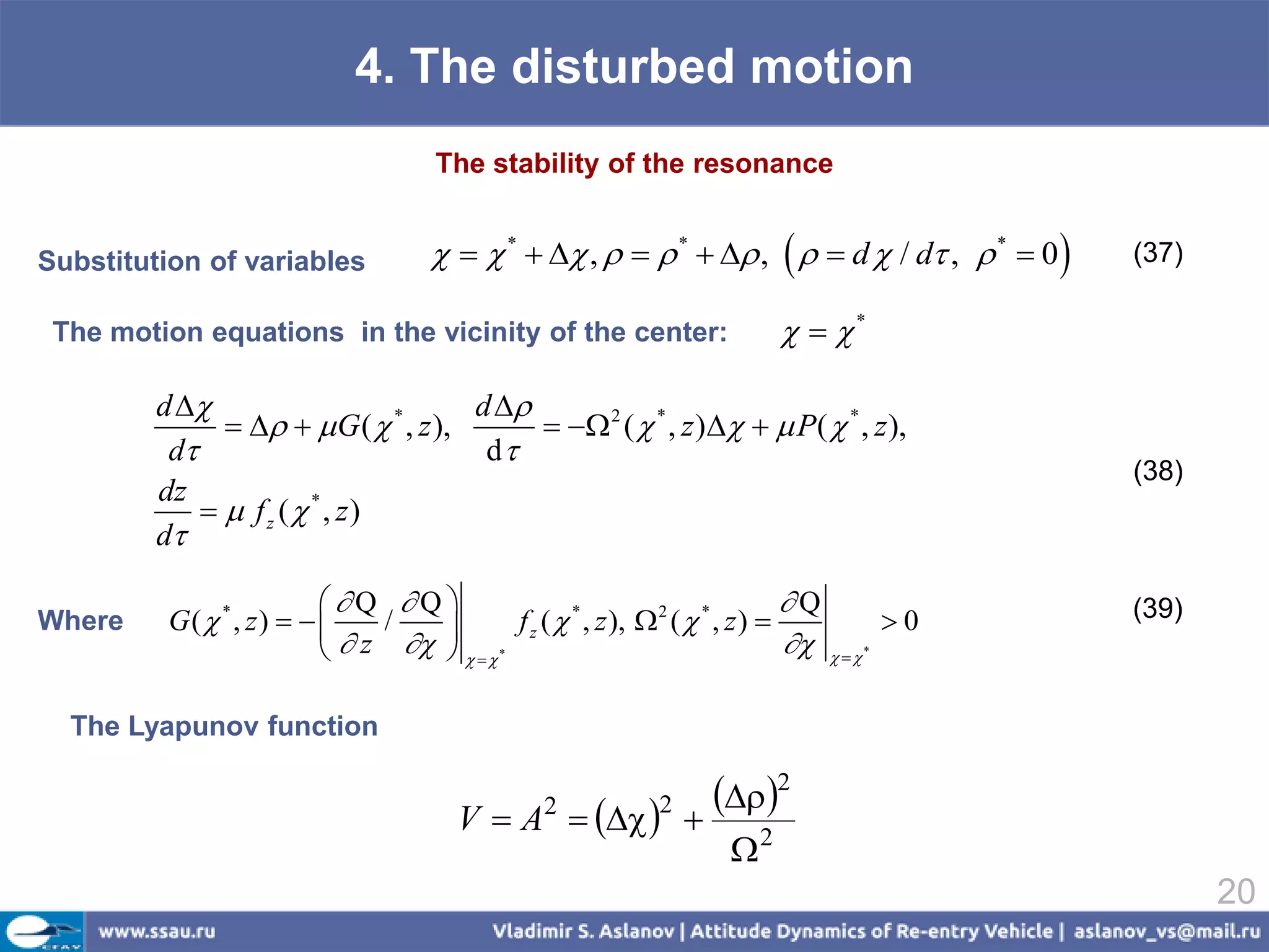
A0-stable; A1,A2 - unstable A0-unstable; A1,A2 - stable
A1,A2 – stable if   
E ( z )  W* or f*  0 (42)
A0 – stable if   
E ( z )  W* or f*  0 (43)
E - average value of the total energy, calculated in neighborhood separatrix
W* - value of the potential energy, calculated at the saddle point u=u*
   
f  f (u , z )  2(1  u 2 )[ E ( z )  W (u , z )]  O( 2 ) (44)
* * * *
23

24. 4. Возмущенное движения
E ( z )  W  m , z  (45)
   m - the amplitude value of the angle of attack
The derivatives by virtue of the averaged equations
 W W W
E ( z)  m 
  z  F ( m , z )   m 
  z
 (46)
   m z   m z   m
 W
W (* , z )  z
 (47)
z  *
The criterion of stability of the disturbed motion in neighborhood the separatrix
m
W (48)
  F ( m , z )   m 
 z

z *
A1,A2 – stable if 0 (49)
A0 – stable if 0 (50)
24

25. 4. The disturbed motion
At the moment of time t* the phase trajectory
intersects the separatrix. Areas A1 and A2 are
stable, therefore the system can continue the
further motion both in area A1, and in area A2.

26. 5. Chaotic oscillations of the RV
Chaotic behavior of an asymmetric body
with the biharmonic moment (classical formulation)
New notation: nutation angle   , inertia moments A  I x , B  I y , C  I z ,
generalized momentums 
p  I x , p  I x R, p  I xG.
B A
Small parameter  (51)
A
(52)
Hamiltonian: H  H 0   H1  O( ) 2
 p  p cos 
2
2 2
p (53)
p
Where H0      a cos   b cos 
2
2A 2 A sin 2  2C
 p  p cos   cos   p sin  sin  
2
H1     (54)
2 A sin 2 
Canonical equations
H H
qi 

pi
, pi  

qi

, qi   ,  , , pi  p , p , p  (55)
26

27. 5. Chaotic oscillations of the RV
Unperturbed system   0  H  H0
  p , p    
p  p cos   p  p cos  
   a sin   b sin 2 ,
A A sin 3 
(56)
p  p  p cos   cos   p  p cos  , p , p  co nst
   ,   
C A sin 2  A sin 2 
The Euler case: a=0, b=0. The Lagrange case: a>0, b=0.
Homoclinic trajectories - separatrices
4
cos  ( j ) (t )  u0  , j  1, 2
2   (4   )C j exp(t )  C j exp( t )
2 1
(57)
27

28. 5. Chaotic oscillations of the RV
Melnikov function

 H 0 H 0 H 0  ( j )
M j  t0     g p  g  g p   (t  t0 ), p (t  t0 ), p ,   t  t0   dt 
( j) ( j)
 
 p  p  (58)

  0 , p   g p  ( j ) (t  t0 ), p ( j ) (t  t0 ), p ,  ( j )  t  t0  dt

Melnikov function for
areas А1 and А2
Where
H1 H H1
g  , g p   1 , g 
p  p
28

29. 5. Chaotic oscillations of the RV
The Poincare sections
Asymmetry  0 Asymmetry   0.01
29

30. 5. Chaotic oscillations of the RV
The Poincare sections
Asymmetry   0.05
30

31. 6. Chaotic oscillations of the Re-entry Vehicle with a
moving center of mass
Mass center of the RV moves along the axis of symmetry
xc  ( xc )0  xc sin(t ) (59)
The motion equation of the RV


 G  R cos   R  G cos    a sin   b sin 2 
sin  3
(60)
  ( a sin   b sin 2 ) sin(t )   m ( )
Melnikov system
    f1  g1 ,

    G  R cos   R  G cos   / sin 3   a sin   b sin 2 

(61)
 (a sin   b sin 2 ) sin    1  sin     f 2  g 2 ,
2

 
31

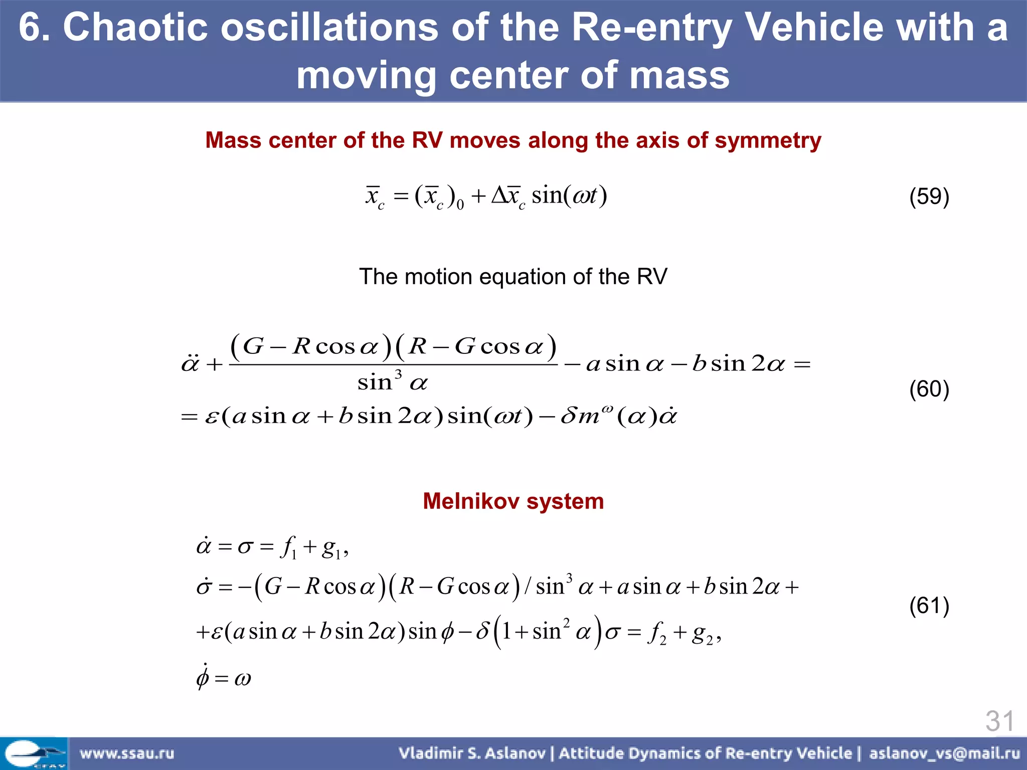
32. 6. Chaotic oscillations of the Re-entry Vehicle with a
moving center of mass
The homoclinic trajectories
4
cos  ( j ) (t )  u0  , j  1, 2 (62)
2   (4   )C j exp(t )  C j exp( t )
2 1
Melnikov function

M (t0 , 0 )   { f1[qi ) (t )] g2[qi ) (t ), t  t0  0 ]}dt  M (i )  M (i )
(i )

( (
(63)


где M      i ) (a sin  i )  b sin 2 i ) ) sin(t  t0  0 )dt ,
(i ) ( ( (

 (64)
M     (1  sin  )( ) dt
(i ) 2 (i )

(i ) 2


The absence condition of the chaos
M(i )  M (i ) (65)
32

33. 6. Chaotic oscillations of the Re-entry Vehicle with a
moving center of mass
The Poincare sections
33

34. 7. Identification of the spacecraft motion by
measuring
7.1. General Terms of the integral method
(66)
The vector of measurements : d  (d1 , d 2 ,.., d m )
The vector of calculated values : g ( )   g1 , g 2, ..., g m  (67)

Where   1 , 2, ..., l  is the vector of estimated parameters

 
N m
The least square method (LSM)   argmin   j d ij  g ij   2 (68)
 i 1 j 1
We know the set of independent first integrals
 
H k ,d j  const, k  1,2,.. p; j  1,2,..m (69)
or the slowly varying functions

dH k ,d j   O (70)
dt
The new criterion
 k  H k  , dij   H k  , gij   
N p 2

  arg min (71)

i 1 k 1
 
34

35. 7. Identification of the spacecraft motion by
measuring
7.2. Identification of the rotational motion of the spacecraft
on the orbit
Measurements of the angular velocity x
d  u ,u ,u
y z  (72)
   x 0 ,  y 0 ,  z 0 , I x , I y , I z 
(73)
The vector of calculated values
The two first integrals depending the angular velocity of
 K x x   y K y   z K z  / 2  H1 ,
(74)
K  K  K  H2
2
x
2
y
2
z

K  I     K x , K y , K z  is the angular momentum, , ,  Are the directional cosines.

The new criterion
 k  H k  ,  uji   H k  ,  jip    , j  x, y, z
N 2 2

  arg min (75)
 
i 1 k 1

35

36. 7. Identification of the spacecraft motion by
measuring
Sample
The number of measurements of the angular velocity N=20
Mathematical expectations and standard deviations of estimates of the
moments of inertia for different measurement intervals t 
The least square method The integral method
t 2 10 25 40 2 10 25 40
MIx 1.499 1.499 1.499 1.493 1.491 1.494 1.499 1.500
I x 0.011 0.009 0.437 0.571 0.082 0.063 0.092 0.074
MIy 5.627 5.619 6.477 7.007 5.604 5.604 5.612 5.605
I y 0.027 0.025 1.651 3.183 0.043 0.046 0.041 0.043
The advantages of the integral method:
1. The accuracy of the method is independent of the measurement step.
2. The method does not require a large number of calculations.
36

37. 7Identification of the spacecraft motion by
measuring
7.3. Identification of the motion of the spacecraft during descent in the
atmosphere

Measurements of the angular velocity and acceleration d  x ,  y , z , nx , n y , nz (76) 
The vector of calculated values:    x0 , D  (77)
x0 is vector the initial conditions,
D are parameters of the spacecraft .
The slowly varying functions:
R  I x x , G
1
n
 I x x nx   y n y   z nz  ,
(78)
1  ci  nx  
n 1 i 1
E  I x x  I  y  I  z  q    
2 2 2
2I 
 i 0 i  1  n  

E is the kinetic energy.
The new criterion
     
N
  argmin   R Riu  Rip   E Eiu  Eip 
~ 2 2 2
 G Giu  Gip (79)
 i 1 
 

37

38. 7. Identification of the spacecraft motion by
measuring
Sample
The number of measurements N=50
Mathematical expectations and standard deviations of estimates of the
stability margin m 
z
t ,c 0.2 2.0 4.0 8.0 16.0
t ,c 0.011 0.105 0.221 0.421 0.842
M m
 -0.0599 -0.0599 -0.0799 - -
z
 m
 0.0006 0.0001 0.0306 - -
z
M ~ -0.0624 -0.0604 -0.0604 -0.0604 -0.0604
mz
 ~ 0.0033 0.0011 0.0011 0.0010 0.0012
mz
K m m
 ~ 0.5264 0.6579 0.0696 - -
z z
The advantages of the integral method:
1. The accuracy of the method is independent of the measurement step.
2. The method does not require a large number of calculations.
38

39. The main results were published in the
following papers and book
• Асланов В.С. Пространственное движение тела в атмосфере, М:. Физматлит, 160 с., 2004.
(Aslanov V.S. Spatial Motion of a Body at Descent in the Atmosphere, Moscow: Fizmatlit, 2004, 160
pages)
• Aslanov V.S. Spatial chaotic vibrations when there is a periodic change in the position of the centre
of mass of a body in the atmosphere- Journal of Applied Mathematics and Mechanics 73 (2009) 179–
187.
• Aslanov V.S. and Ledkov A.S. Analysis of the resonance and ways of its elimination at the descent
of spacecrafts in the rarefied atmosphere - Aerospace Science and Technology 13 (2009) 224–231.
• Aslanov V.S. Resonance at motion of a body in the Mars’s atmosphere under biharmonical moment -
WSEAS TRANSACTIONS on SYSTEMS AND CONTROL, Issue 1, Volume 3, January 2008, (ISSN:
1991-8763), pp. 33-39.
• Aslanov V. S. and Doroshin A. V. Influence of Disturbances on the Angular Motion of a Spacecraft in
the Powered Section of Its Descent - Cosmic Research ISSN 0010-9525, Vol. 46, No. 2, 2008, pp. 166-
171.
• Aslanov V.S. Resonance at Descent in the Mars’s Atmosphere of Analogue of the Beagle 2 Lander -
Proceedings of 3rd WSEAS International Conference on DYNAMICAL SYSTEMS and CONTROL
(CONTROL'07), Arcachon, France, October 13-15, 2007, 178-181.
• Aslanov V. S. and Ledkov A.S. Features of Rotational Motion of a Spacecraft Descending in the
Martian Atmosphere - Cosmic Research ISSN 0010-9525, 2007, Vol. 45, No. 4, 331-337.
• Aslanov V. S. Doroshin A. V. and Kruglov G.E. The mothion of coaxial bodies of varying
composition on the active leg of descent - Cosmic Research ISSN 0010-9525, Vol. 43, No. 3, 2005, pp.
213-221.
39

40. The main results were published in the
following papers and book
• Aslanov V. S. The motion of a rotating body in a resisting medium - Mechanics of Solids, 2005, vol.
40, no2, pp. 21-32.
• Aslanov V.S. and Timbyi I.A. Action-angle canonical variables for the motion of a rigid body under
the action of a biharmonic torque - Mechanics of Solids, Vol. 38, No. 1, pp. 13-23, 2003.
• Aslanov V. S. and Doroshin A. V. Stabilization of a Reentry Vehicle by a Partial Spin-up during
Uncontrolled Descent - Cosmic Research ISSN 0010-9525, Vol. 40, No. 2, 2002, pp. 178-185.
• Aslanov V. S. and Myasnikov S. V. Analysis of Nonlinear Resonances during Spacecraft Descent in
the Atmosphere - Cosmic Research ISSN 0010-9525, Vol. 35, No. 6, 1997, pp. 616-622.
• Aslanov V. S. and Timbay I. A. Transient Modes of Spacecraft Angular Motion on the Upper Section
of the Reentry Trajectory - Cosmic Research ISSN 0010-9525, Vol. 35, No. 3, 1997, pp. 260-267.
• Aslanov V. S. and Myasnikov S. V. Stability of Nonlinear Resonance Modes of Spacecraft Motion in
the Atmosphere - Cosmic Research ISSN 0010-9525, Vol. 34, No. 6, 1996, pp. 579-584.
• Aslanov V. S. and Timbay I. A. Some Problem of the Reentry Vehicles Dynamics- Cosmic Research
ISSN 0010-9525, Vol. 33, No. 6, 1995.
• Aslanov V.S. Nonlinear Resonances of the Slightly Asymmetric Reentry Vehicles - Cosmic
Research ISSN 0010-9525, Vol. 30, No. 5, 1992.
• Aslanov V.S. Definition of Rotary Movement of a Space Vehicle by Results of Measurements -
Cosmic Research ISSN 0010-9525, Vol. 27, No. 3, 1989.
• Aslanov V.S. Two Kinds of Nonlinear Resonant Movement of an Asymmetric Reentry Vehicle -
Cosmic Research ISSN 0010-9525, Vol. 26, No. 2, 1988.
• Aslanov V. S. and Boyko V.V. Nonlinear Resonant Movement of an Asymmetric Reentry Vehicle -
Cosmic Research ISSN 0010-9525, Vol. 23, No. 3, 1985.
40

41. The main results were published in the
following papers and book
• Aslanov V. S., Boyko V.V. and Timbay I. A. Spatial Fluctuations of the Symmetric Reentry Vehicle at
Any Corners of Attack - Cosmic Research ISSN 0010-9525, Vol. 19, No. 5, 1981.
• Aslanov V. S. Definition of Amplitude of Spatial Fluctuations of the Slightly Asymmetric Reentry
Vehicles - Cosmic Research ISSN 0010-9525, Vol. 18, No. 2, 1980.
• Aslanov V. S. About Rotary Movement of the Symmetric Reentry Vehicle - Cosmic Research ISSN
0010-9525, Vol. 14, No. 4, 1976.
41