Appendex d

October 22, 2004 12:43 k34-appd Sheet number 1 Page number 31 cyan magenta yellow black
PAGE PROOFS
A31
a p p e n d i x d
REAL NUMBERS, INTERVALS,
AND INEQUALITIES
REAL NUMBERS
Figure D.1 describes the various categories of numbers that we will encounter in this text.
The simplest numbers are the natural numbers
1, 2, 3, 4, 5, . . .
These are a subset of the integers
. . . , −4, −3, −2, −1, 0, 1, 2, 3, 4, . . .
and these in turn are a subset of the rational numbers, which are the numbers formed by
taking ratios of integers (avoiding division by 0). Some examples are
2
3
, 7
5
, 23 = 23
1
, 0.19 = 19
100
, −5
2
= −5
2
= 5
−2
Complex numbers:
a + bi, where i = √–1
Real numbers:
Rational and irrational numbers
Integers:
..., –4, –3, –2, –1, 0, 1, 2, 3, 4, ...
Natural numbers:
1, 2, 3, 4, 5, ...
Rational
numbers:
2
3
7
5
23
1
5
2
–, , , 0.19,
Figure D.1
The early Greeks believed that every measurable quantity had to be a rational number.
However, this idea was overturned in the ﬁfth century B.C. by Hippasus of Metapontum
who demonstrated the existence of irrational numbers, that is, numbers that cannot be
expressed as the ratio of two integers. Using geometric methods, he showed that the length
of the hypotenuse of the triangle in Figure D.2 could not be expressed as a ratio of integers,
thereby proving that
√
2 is an irrational number. Some other examples of irrational numbers
are √
3,
√
5, 1 +
√
2,
3√
7, π, cos 19◦
Therationalandirrationalnumberstogethercomprisewhatiscalledtherealnumbersystem,
and both the rational and irrational numbers are called real numbers.
Hippasus of Metapon-
tum (circa 500 B.C.)
A Greek Pythagorean
philosopher. Accord-
ing to legend, Hippasus
made his discovery
at sea and was thrown overboard
by fanatic Pythagoreans because
his result contradicted their doc-
trine. The discovery of Hippasus
is one of the most fundamental in
the entire history of science.
1
1
√2
Figure D.2
COMPLEX NUMBERS
Because the square of a real number cannot be negative, the equation
x2
= −1
has no solutions in the real number system. In the eighteenth century mathematicians
remedied this problem by inventing a new number, which they denoted by
i =
√
−1
and which they deﬁned to have the property i2
= −1. This, in turn, led to the development
of the complex numbers, which are numbers of the form
a + bi
where a and b are real numbers. Some examples are
2 + 3i 3 − 4i 6i 2
3
|a = 2, b = 3| |a = 3, b = −4| |a = 0, b = 6| |a = 2
3 , b = 0|
Observe that every real number a is also a complex number because it can be written as
a = a + 0i

PAGE PROOFS
A32 Appendix D: Real Numbers, Intervals, and Inequalities
Thus, the real numbers are a subset of the complex numbers. Although we will be concerned
primarily with real numbers in this text, complex numbers will arise in the course of solving
equations. For example, the solutions of the quadratic equation
ax2
+ bx + c = 0
which are given by the quadratic formula
x =
−b ±
√
b2 − 4ac
2a
are not real if the quantity b2
− 4ac is negative.
DIVISION BY ZERO
Division by zero is not allowed in numerical computations because it leads to mathematical
inconsistencies. For example, if 1/0 were assigned some numerical value, say p, then it
would follow that 0 · p = 1, which is incorrect.
DECIMAL REPRESENTATION OF REAL NUMBERS
Rational and irrational numbers can be distinguished by their decimal representations. Ra-
tional numbers have decimals that are repeating, by which we mean that at some point in
the decimal some ﬁxed block of numbers begins to repeat indeﬁnitely. For example,
4
3
= 1.333 . . . ,
3 repeats
3
11
= .272727 . . . ,
27 repeats
1
2
= .50000 . . . ,
0 repeats
5
7
= .714285714285714285 . . .
714285 repeats
Decimals in which zero repeats from some point on are called terminating decimals. For
brevity, it is usual to omit the repetitive zeros in terminating decimals and for other repeating
decimals to write the repeating digits only once but with a bar over them to indicate the repe-
tition. For example,
1
2
= .5, 12
4
= 3, 8
25
= .32, 4
3
= 1.3, 3
11
= .27, 5
7
= .714285
Irrational numbers have nonrepeating decimals, so we can be certain that the decimals
√
2 = 1.414213562373095 . . . and π = 3.141592653589793 . . .
do not repeat from some point on. Moreover, if we stop the decimal expansion of an
irrational number at some point, we get only an approximation to the number, never an
exact value. For example, even if we compute π to 1000 decimal places, as in Figure D.3,
we still have only an approximation.
3.141592653589793238462643383279502884197169
39937510582097494459230781640628620899862803
48253421170679821480865132823066470938446095
50582231725359408128481117450284102701938521
10555964462294895493038196442881097566593344
61284756482337867831652712019091456485669234
60348610454326648213393607260249141273724587
00660631558817488152092096282925409171536436
78925903600113305305488204665213841469519415
11609433057270365759591953092186117381932611
79310511854807446237996274956735188575272489
12279381830119491298336733624406566430860213
94946395224737190702179860943702770539217176
29317675238467481846766940513200056812714526
35608277857713427577896091736371787214684409
01224953430146549585371050792279689258923542
01995611212902196086403441815981362977477130
99605187072113499999983729780499510597317328
16096318595024459455346908302642522308253344
68503526193118817101000313783875288658753320
83814206171776691473035982534904287554687311
59562863882353787593751957781857780532171226
8066130019278766111959092164201989
Figure D.3
Beginning mathematics students are sometimes taught to approximate π by 22
7
. Keep in mind,
however, that this is only an approximation, since
22
7
= 3.142857
is a rational number whose decimal representation begins to differ from π in the third decimal
place.
COORDINATE LINES
In 1637 René Descartes published a philosophical work called Discourse on the Method
of Rightly Conducting the Reason. In the back of that book was an appendix that the Brit-
ish philosopher John Stuart Mill described as “the greatest single step ever made in the
progress of the exact sciences.” In that appendix René Descartes linked together algebra
and geometry, thereby creating a new subject called analytic geometry; it gave a way of
describing algebraic formulas by geometric curves and, conversely, geometric curves by
algebraic formulas.

PAGE PROOFS
Appendix D: Real Numbers, Intervals, and Inequalities A33
The key step in analytic geometry is to establish a correspondence between real numbers
and points on a line. To do this, choose any point on the line as a reference point, and call
it the origin; and then arbitrarily choose one of the two directions along the line to be the
positive direction, and let the other be the negative direction. It is usual to mark the positive
direction with an arrowhead, as in Figure D.4, and to take the positive direction to the right
when the line is horizontal. Next, choose a convenient unit of measure, and represent each
positive number r by the point that is r units from the origin in the positive direction, each
negative number −r by the point that is r units from the origin in the negative direction
from the origin, and 0 by the origin itself (Figure D.5). The number associated with a point
P is called the coordinate of P, and the line is called a coordinate line, a real number line,
or a real line.
Origin +–
Figure D.4
Figure D.5 -4 -3 -2 -1 0 1 2 3 4
-1.75 c2
1
-
√2
INEQUALITY NOTATION
The real numbers can be ordered by size as follows: If b − a is positive, then we write
either a a (read “b is greater than a”). We write a ≤ b
to mean a < b or a = b, and we write a < b < c to mean that a < b and b < c. As one
traverses a coordinate line in the positive direction, the real numbers increase in size, so
on a horizontal coordinate line the inequality a < b implies that a is to the left of b, and
the inequalities a < b < c imply that a is to the left of c, and b lies between a and c. The
meanings of such symbols as
a ≤ b < c, a ≤ b ≤ c, and a −7, −π > −12, 5 ≥ 5, 3 > 0 > −1 > −3
REVIEW OF SETS
In the following discussion we will be concerned with certain sets of real numbers, so it will
be helpful to review the basic ideas about sets. Recall that a set is a collection of objects,
called elements or members of the set. In this text we will be concerned primarily with sets
whose members are numbers or points that lie on a line, a plane, or in three-dimensional
space. We will denote sets by capital letters and elements by lowercase letters. To indicate
that a is a member of the set A we will write a ∈ A (read “a belongs to A”), and to indicate
that a is not a member of the set A we will write a /∈ A (read “a does not belong to A”).
For example, if A is the set of positive integers, then 5 ∈ A, but −5 /∈ A. Sometimes sets
René Descartes (1596–1650) Descartes, a French aristo-
crat, was the son of a government official. He graduated
from the University of Poitiers with a law degree at age 20.
After a brief probe into the pleasures of Paris he became
a military engineer, first for the Dutch Prince of Nassau
and then for the German Duke of Bavaria. It was dur-
ing his service as a soldier that Descartes began to pursue mathemat-
ics seriously and develop his analytic geometry. After the wars, he
returned to Paris where he stalked the city as an eccentric, wearing
a sword in his belt and a plumed hat. He lived in leisure, seldom
arose before 11 D.M., and dabbled in the study of human physiology,
philosophy, glaciers, meteors, and rainbows. He eventually moved
to Holland, where he published his Discourse on the Method, and
finally to Sweden where he died while serving as tutor to Queen
Christina. Descartes is regarded as a genius of the first magnitude.
In addition to major contributions in mathematics and philosophy,
he is considered, along with William Harvey, to be a founder of
modern physiology.

PAGE PROOFS
arise that have no members (e.g., the set of odd integers that are divisible by 2). A set with
no members is called an empty set or a null set and is denoted by the symbol л.
Some sets can be described by listing their members between braces. The order in which
the members are listed does not matter, so, for example, the set A of positive integers that
are less than 6 can be expressed as
A = {1, 2, 3, 4, 5} or A = {2, 3, 1, 5, 4}
We can also write A in set-builder notation as
A = {x : x is an integer and 0 < x < 6}
which is read “A is the set of all x such that x is an integer and 0 < x < 6.” In general,
to express a set S in set-builder notation we write S = {x : } in which the line is
replaced by a property that identifies exactly those elements in the set S.
If every member of a set A is also a member of a set B, then we say that A is a subset
of B and write A ⊆ B. For example, if A is the set of positive integers and B is the set
of all integers, then A ⊆ B. If two sets A and B have the same members (i.e., A ⊆ B and
B ⊆ A), then we say that A and B are equal and write A = B.
INTERVALS
In calculus we will be concerned with sets of real numbers, called intervals, that correspond
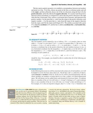
to line segments on a coordinate line. For example, if a < b, then the open interval from a
to b, denoted by (a, b), is the line segment extending from a to b, excluding the endpoints;
and the closed interval from a to b, denoted by [a, b], is the line segment extending from
a to b, including the endpoints (Figure D.6). These sets can be expressed in set-builder
notation as
(a, b) = {x : a < x < b} The open interval from a to b
[a, b] = {x : a ≤ x ≤ b} The closed interval from a to b
a b
a b
The open interval (a, b)
The closed interval [a, b]
Figure D.6
Observe that in this notation and in the corresponding Figure D.6, parentheses and open dots mark
endpoints that are excluded from the interval, whereas brackets and closed dots mark endpoints
that are included in the interval. Observe also that in set-builder notation for the intervals, it is
understood that x is a real number, even though it is not stated explicitly.
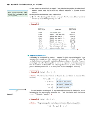
As shown in Table 1, an interval can include one endpoint and not the other; such
intervals are called half-open (or sometimes half-closed). Moreover, the table also shows
that it is possible for an interval to extend indefinitely in one or both directions. To indicate
that an interval extends indefinitely in the positive direction we write +ϱ (read “positive
infinity”) in place of a right endpoint, and to indicate that an interval extends indefinitely
in the negative direction we write −ϱ (read “negative infinity”) in place of a left endpoint.
Intervals that extend between two real numbers are called finite intervals, whereas intervals
that extend indefinitely in one or both directions are called infinite intervals.
By convention, infinite intervals of the form [a, +ϱ) or (−ϱ, b] are considered to be closed because
they contain their endpoint, and intervals of the form (a, +ϱ) and (−ϱ, b) are considered to be
open because they do not include their endpoint. The interval (−ϱ, +ϱ), which is the set of all real
numbers, has no endpoints and can be regarded as both open and closed. This set is often denoted
by the special symbol R. To distinguish verbally between the open interval (0, +ϱ) = {x : x > 0}
and the closed interval [0, +ϱ) = {x : x ≥ 0}, we will call x positive if x > 0 and nonnegative if x ≥ 0.
Thus, a positive number must be nonnegative, but a nonnegative number need not be positive,
since it might possibly be 0.

PAGE PROOFS
Table 1
a b
a b
a b
a b
b
b
a
a
interval
notation
set
notation
geometric
picture
(a, b)
[a, b]
[a, b)
(a, b]
(–∞, b]
(–∞, b)
[a, +∞)
(a, +∞)
(–∞, +∞)
Finite; open
Finite; closed
Finite; half-open
Finite; half-open
Infinite; closed
Infinite; open
Infinite; closed
Infinite; open
Infinite; open and closed
{x : a < x < b}
{x : a ≤ x ≤ b}
{x : a ≤ x < b}
{x : a < x ≤ b}
{x : x ≤ b}
{x : x < b}
{x : x ≥ a}
{x : x > a}
classification
UNIONS AND INTERSECTIONS OF INTERVALS
If A and B are sets, then the union of A and B (denoted by A ∪ B) is the set whose members
belong to A or B (or both), and the intersection of A and B (denoted by A ∩ B) is the set
whose members belong to both A and B. For example,
{x : 0 < x < 5} ∪ {x : 1 < x < 7} = {x : 0 < x < 7}
{x : x < 1} ∩ {x : x ≥ 0} = {x : 0 ≤ x < 1}
{x : x < 0} ∩ {x : x > 0} = л
or in interval notation, (0, 5) ∪ (1, 7) = (0, 7)
(−ϱ, 1) ∩ [0, +ϱ) = [0, 1)
(−ϱ, 0) ∩ (0, +ϱ) = л
ALGEBRAIC PROPERTIES OF INEQUALITIES
The following algebraic properties of inequalities will be used frequently in this text. We
omit the proofs.
D.1 theorem (Properties of Inequalities). Let a, b, c, and d be real numbers.
(a) If a bc when c is negative.
(d) If a 1/b.
If we call the direction of an inequality its sense, then these properties can be paraphrased
as follows:
(b) The sense of an inequality is unchanged if the same number is added to or subtracted
from both sides.

PAGE PROOFS
(c) The sense of an inequality is unchanged if both sides are multiplied by the same positive
number, but the sense is reversed if both sides are multiplied by the same negative
number.
(d) Inequalities with the same sense can be added.
(e) If both sides of an inequality have the same sign, then the sense of the inequality is
reversed by taking the reciprocal of each side.
These properties remain true if the
symbols < and > are replaced by ≤ and
≥ in Theorem D.1.
Example 1
starting
inequality
resulting
inequality
Add 7 to both sides.
Subtract 8 from both sides.
Multiply both sides by 3.
Multiply both sides by –3.
Multiply both sides by 4.
Multiply both sides by –4.
Take reciprocals of both sides.
Take reciprocals of both sides.
Add corresponding sides.
operation
–2 < 6
–2 < 6
–2 < 6
–2 < 6
3 < 7
3 < 7
3 < 7
–8 < –6
4 < 5, –7 < 8
5 < 13
–10 < –2
–6 < 18
12 < 28
–12 > –28
1
3
1
7
>
1
8
1
6
>– –
6 > –18
–3 < 13
SOLVING INEQUALITIES
A solution of an inequality in an unknown x is a value for x that makes the inequality a true
statement. For example, x = 1 is a solution of the inequality x < 5, but x = 7 is not. The
set of all solutions of an inequality is called its solution set. It can be shown that if one does
not multiply both sides of an inequality by zero or an expression involving an unknown,
then the operations in Theorem D.1 will not change the solution set of the inequality. The
process of ﬁnding the solution set of an inequality is called solving the inequality.
Example 2 Solve 3 + 7x ≤ 2x − 9.
Solution. We will use the operations of Theorem D.1 to isolate x on one side of the
inequality.
3 + 7x ≤ 2x − 9 Given.
7x ≤ 2x − 12 We subtracted 3 from both sides.
5x ≤ −12 We subtracted 2x from both sides.
x ≤ −12
5
We multiplied both sides by 1
5 .
Because we have not multiplied by any expressions involving the unknown x, the last
inequality has the same solution set as the ﬁrst. Thus, the solution set is the interval
−ϱ, −12
5
shown in Figure D.7.
12
5
–
Figure D.7
Example 3 Solve 7 ≤ 2 − 5x < 9.
Solution. The given inequality is actually a combination of the two inequalities
7 ≤ 2 − 5x and 2 − 5x < 9

PAGE PROOFS
We could solve the two inequalities separately, then determine the values of x that satisfy
both by taking the intersection of the two solution sets. However, it is possible to work
with the combined inequalities in this problem:
7 ≤ 2 − 5x < 9 Given.
5 ≤ −5x < 7 We subtracted 2 from each member.
−1 ≥ x > −
7
5
We multiplied by − 1
5 and reversed
the sense of the inequalities.
−
7
5
< x ≤ −1 For clarity, we rewrote the inequalities
with the smaller number on the left.
Thus, the solution set is the interval −7
5
, −1 shown in Figure D.8.
7
5
– –1
Figure D.8
Example 4 Solve x2
− 3x > 10.
Solution. By subtracting 10 from both sides, the inequality can be rewritten as
x2
− 3x − 10 > 0
Factoring the left side yields
(x + 2)(x − 5) > 0
The values of x for which x + 2 = 0 or x − 5 = 0 are x = −2 and x = 5. These points
divide the coordinate line into three open intervals,
(−ϱ, −2), (−2, 5), (5, +ϱ)
on each of which the product (x + 2)(x − 5) has constant sign. To determine those signs
we will choose an arbitrary point in each interval at which we will determine the sign; these
are called test points. As shown in Figure D.9, we will use −3, 0, and 6 as our test points.
The results can be organized as follows:
sign of
(x + 2)(x – 5)
at the test point
–3
0
6
test pointinterval
(–∞, –2)
(–2, 5)
(5, +∞)
(–)(–) = +
(+)(–) = –
(+)(+) = +
The pattern of signs in the intervals is shown on the number line in the middle of Figure D.9.
We deduce that the solution set is (−ϱ, −2) ∪ (5, +ϱ), which is shown at the bottom of
Figure D.9.
Figure D.9 –2 5
–2
–2
5
5
–3 0 6
0 0– – – – – – + + + ++ + +
Test points
Sign of (x + 2)(x – 5)
Solution set for
(x + 2)(x – 5) > 0

PAGE PROOFS
Example 5 Solve
2x − 5
x − 2
< 1.
Solution. We could start by multiplying both sides by x − 2 to eliminate the fraction.
However, this would require us to consider the cases x − 2 > 0 and x − 2 < 0 separately
because the sense of the inequality would be reversed in the second case, but not the first.
The following approach is simpler:2x − 5
x − 2
< 1 Given.
2x − 5
x − 2
− 1 < 0 We subtracted 1 from both sides
to obtain a 0 on the right.
(2x − 5) − (x − 2)
x − 2
< 0 We combined terms.
x − 3
x − 2
< 0 We simplified.
The quantity x − 3 is zero if x = 3, and the quantity x − 2 is zero if x = 2. These points
divide the coordinate line into three open intervals,
(−ϱ, 2), (2, 3), (3, +ϱ)
on each of which the quotient (x − 3)/(x − 2) has constant sign. Using 0, 2.5, and 4 as
test points (Figure D.10), we obtain the following results:
sign of
(x – 3)/(x – 2)
at the test point
0
2.5
4
test pointinterval
(–∞, 2)
(2, 3)
(3, +∞)
(–)/(–) = +
(–)/(+) = –
(+)/(+) = +
The signs of the quotient are shown in the middle of Figure D.10. From the figure we see
that the solution set consists of all real values of x such that 2 < x < 3. This is the interval
(2, 3) shown at the bottom of Figure D.10.
Figure D.10
2 3
2 3
2 3
0 2.5 4
0– + + + ++ + +
Solution set for
+++ + + –
Sign of
x – 2
x – 3
x – 2
x – 3
Test points
< 0
EXERCISE SET D
1. Among the terms integer, rational, and irrational, which
ones apply to the given number?
(a) −3
4
(b) 0 (c) 24
8
(d) 0.25
(e) −
√
16 (f ) 21/2
(g) 0.020202 . . . (h) 7.000 . . .
2. Which of the terms integer, rational, and irrational apply
to the given number?
(a) 0.31311311131111 . . . (b) 0.729999 . . .
(c) 0.376237623762 . . . (d) 174
5

PAGE PROOFS
3. The repeating decimal 0.137137137 . . . can be expressed as
a ratio of integers by writing
x = 0.137137137 . . .
1000x = 137.137137137 . . .
and subtracting to obtain 999x = 137 or x = 137
999
. Use this
idea, where needed, to express the following decimals as
ratios of integers.
(a) 0.123123123 . . . (b) 12.7777 . . .
(c) 38.07818181 . . . (d) 0.4296000 . . .
4. Show that the repeating decimal 0.99999 . . . represents the
number 1. Since 1.000 . . . is also a decimal representation
of 1, this problem shows that a real number can have two
different decimal representations. [Hint: Use the technique
of Exercise 3.]
5. The Rhind Papyrus, which is a fragment of Egyptian math-
ematical writing from about 1650 B.C., is one of the oldest
known examples of written mathematics. It is stated in the
papyrus that the area A of a circle is related to its diameter
D by
A = 8
9
D
2
(a) What approximation to π were the Egyptians using?
(b) Use a calculating utility to determine if this approxi-
mation is better or worse than the approximation 22
7
.
6. The following are all famous approximations to π:
333
106
Adrian Athoniszoon, c. 1583
355
113
Tsu Chung-Chi and others
63
25
17 + 15
√
5
7 + 15
√
5
Ramanujan
22
7
Archimedes
223
71
Archimedes
(a) Use a calculating utility to order these approximations
according to size.
(b) Which of these approximations is closest to but larger
than π?
(c) Which of these approximations is closest to but smaller
than π?
(d) Which of these approximations is most accurate?
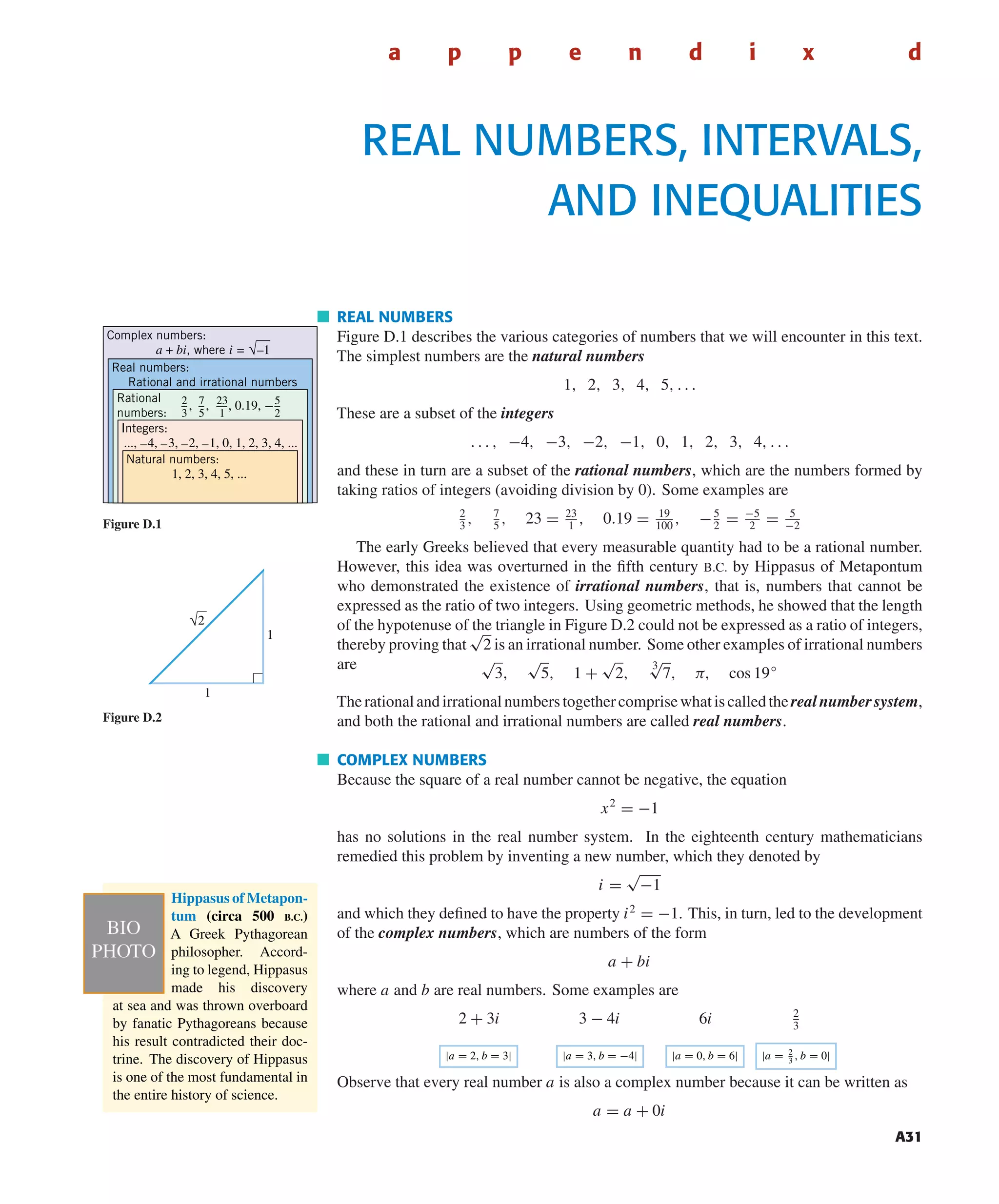
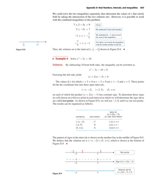
7. In each line of the accompanying table, check the blocks,
if any, that describe a valid relationship between the real
numbers a and b. The ﬁrst line is already completed as an
illustration.
a
1
6
–3
5
–4
0.25
6
1
5
–3
–4
b a b a ≥ b a = b
4
1
4
3
3
1
––
Table Ex-7
8. In each line of the accompanying table, check the blocks,
if any, that describe a valid relationship between the real
numbers a, b, and c.
a
–1
2
–5
0.75
0
4
–5
1.25
2
–3
–5
1.25
b c a < b < c a ≤ b ≤ c a < b ≤ c a ≤ b < c
2
1
2
1
4
3
Table Ex-8
9. Which of the following are always correct if a ≤ b?
(a) a − 3 ≤ b − 3 (b) −a ≤ −b (c) 3 − a ≤ 3 − b
(d) 6a ≤ 6b (e) a2
≤ ab (f ) a3
≤ a2
b
10. Which of the following are always correct if a ≤ b and
c ≤ d?
(a) a + 2c ≤ b + 2d (b) a − 2c ≤ b − 2d
(c) a − 2c ≥ b − 2d
11. For what values of a are the following inequalities valid?
(a) a ≤ a (b) a < a
12. If a ≤ b and b ≤ a, what can you say about a and b?
13. (a) If a < b is true, does it follow that a ≤ b must also be
true?
(b) If a ≤ b is true, does it follow that a < b must also be
true?
14. In each part, list the elements in the set.
(a) {x : x2
− 5x = 0}
(b) {x : x is an integer satisfying −2 < x < 3}
15. In each part, express the set in the notation {x : }.
(a) {1, 3, 5, 7, 9, . . .}
(b) the set of even integers
(c) the set of irrational numbers
(d) {7, 8, 9, 10}
16. Let A = {1, 2, 3}. Which of the following sets are equal
to A?
(a) {0, 1, 2, 3} (b) {3, 2, 1}
(c) {x : (x − 3)(x2
− 3x + 2) = 0}

PAGE PROOFS
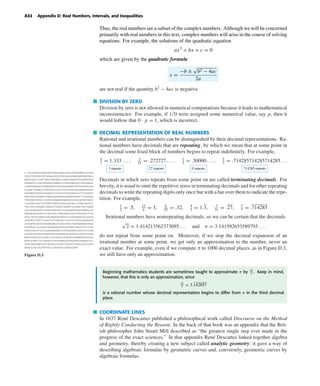
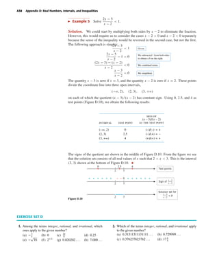
17. In the accompanying ﬁgure, let
S = the set of points inside the square
T = the set of points inside the triangle
C = the set of points inside the circle
and let a, b, and c be the points shown. Answer the follow-
ing as true or false.
(a) T ⊆ C (b) T ⊆ S
(c) a /∈ T (d) a /∈ S
(e) b ∈ T and b ∈ C (f ) a ∈ C or a ∈ T
(g) c ∈ T and c /∈ C
c
b
a
Figure Ex-17
18. List all subsets of
(a) {a1, a2, a3} (b) л.
19. In each part, sketch on a coordinate line all values of x that
satisfy the stated condition.
(a) x ≤ 4 (b) x ≥ −3 (c) −1 ≤ x ≤ 7
(d) x2
= 9 (e) x2
≤ 9 (f ) x2
≥ 9
20. In parts (a)–(d), sketch on a coordinate line all values of x,
if any, that satisfy the stated conditions.
(a) x > 4 and x ≤ 8
(b) x ≤ 2 or x ≥ 5
(c) x > −2 and x ≥ 3
(d) x ≤ 5 and x > 7
21. Express in interval notation.
(a) {x : x2
≤ 4} (b) {x : x2
> 4}
22. In each part, sketch the set on a coordinate line.
(a) [−3, 2] ∪ [1, 4] (b) [4, 6] ∪ [8, 11]
(c) (−4, 0) ∪ (−5, 1) (d) [2, 4) ∪ (4, 7)
(e) (−2, 4) ∩ (0, 5] (f ) [1, 2.3) ∪ (1.4,
√
2)
(g) (−ϱ, −1) ∪ (−3, +ϱ) (h) (−ϱ, 5) ∩ [0, +ϱ)
23–44 Solve the inequality and sketch the solution on a co-
ordinate line.
23. 3x − 2 < 8 24. 1
5
x + 6 ≥ 14
25. 4 + 5x ≤ 3x − 7 26. 2x − 1 > 11x + 9
27. 3 ≤ 4 − 2x < 7 28. −2 ≥ 3 − 8x ≥ −11
29.
x
x − 3
< 4 30.
x
8 − x
≥ −2
31.
3x + 1
x − 2
< 1 32.
1
2
x − 3
4 + x
> 1
33.
4
2 − x
≤ 1 34.
3
x − 5
≤ 2
35. x2
> 9 36. x2
≤ 5
37. (x − 4)(x + 2) > 0 38. (x − 3)(x + 4) < 0
39. x2
− 9x + 20 ≤ 0 40. 2 − 3x + x2
≥ 0
41.
2
x
<
3
x − 4
42.
1
x + 1
≥
3
x − 2
43. x3
− x2
− x − 2 > 0 44. x3
− 3x + 2 ≤ 0
45–46 Find all values of x for which the given expression
yields a real number.
45.
√
x2 + x − 6 46.
x + 2
x − 1
47. Fahrenheit and Celsius temperatures are related by the for-
mula C = 5
9
(F − 32). If the temperature in degrees Celsius
ranges over the interval 25 ≤ C ≤ 40 on a certain day, what
is the temperature range in degrees Fahrenheit that day?
48. Every integer is either even or odd. The even integers are
those that are divisible by 2, so n is even if and only if
n = 2k for some integer k. Each odd integer is one unit
larger than an even integer, so n is odd if and only if
n = 2k + 1 for some integer k. Show:
(a) If n is even, then so is n2
(b) If n is odd, then so is n2
.
49. Prove the following results about sums of rational and
irrational numbers:
(a) rational + rational = rational
(b) rational + irrational = irrational.
50. Prove the following results about products of rational and
irrational numbers:
(a) rational · rational = rational
(b) rational · irrational = irrational (provided the rational
factor is nonzero).
51. Show that the sum or product of two irrational numbers can
be rational or irrational.
52. Classify the following as rational or irrational and justify
your conclusion.
(a) 3 + π (b) 3
4
√
2 (c)
√
8
√
2 (d)
√
π
(See Exercises 49 and 50.)
53. Prove: The average of two rational numbers is a rational
number, but the average of two irrational numbers can be
rational or irrational.
54. Can a rational number satisfy 10x
= 3?
55. Solve: 8x3
− 4x2
− 2x + 1 < 0.
56. Solve: 12x3
− 20x2
≥ −11x + 2.
57. Prove: If a, b, c, and d are positive numbers such that a < b
and c < d, then ac < bd. (This result gives conditions un-
der which inequalities can be “multiplied together.”)
58. Is the number represented by the decimal
0.101001000100001000001 . . .
rational or irrational? Explain your reasoning.

Appendex d

Recommended

Recommended

More Related Content

What's hot

What's hot (19)

Viewers also liked

Viewers also liked (20)

Similar to Appendex d

Similar to Appendex d (20)

More from swavicky

More from swavicky (10)

Appendex d