The document discusses Catalan numbers and provides several problems that are equivalent in that they all generate the same sequence of numbers called the Catalan numbers. It introduces problems involving balanced parentheses, mountain ranges, diagonal-avoiding paths, polygon triangulations, handshakes around a table, binary trees, and more. It then derives a recursive definition for the Catalan numbers by analyzing the balanced parentheses problem and showing the number of configurations for n pairs is equal to the sum of configurations of i pairs times configurations of n-i-1 pairs, for i from 0 to n-1. Finally, it shows this same recursive relationship holds for the polygon triangulations and non-crossing handshake problems.
Interaction of xrays and gamma rays with matter iiSneha George
The document discusses four main mechanisms by which photons interact with matter: coherent scattering, photoelectric effect, Compton scattering, and pair production. It provides details on each mechanism, noting that the photoelectric effect dominates at low energies, pair production at very high energies above 1 MeV, and Compton scattering is predominant at medium energies. It also discusses absorption and transmission of photons in materials, how attenuation coefficients vary with photon energy and material properties like atomic number, and the spatial distribution of secondary radiation produced.
Presentation contains info on Radiation Protection in Pregnancy - radiodiagnosis, MRI, nuclear medicine and radiotherapy. Including notes on foetal dose, shielding techniques in radiotherapy and precaution for pregnant radiographers/medical physicists.
This document discusses the imaging modalities and indications for imaging patients presenting with acute abdominal pain. It covers plain abdominal radiographs, ultrasound, and CT scanning. For each modality, it outlines the specific indications and conditions they are best used for in evaluating abdominal pain, such as suspected bowel obstructions, appendicitis, diverticulitis, and others. The document provides examples of imaging findings for various acute abdominal pathologies.
Radiologic imaging during pregnancy has increased over the last 10 years. The document discusses the risks of radiation exposure to fetuses from various medical imaging procedures. It finds that deterministic effects require a threshold dose above 10 rads but stochastic effects have no threshold. Common procedures like x-rays present minimal risk while CT scans can double cancer risk for doses over 2-5 rads. MRI is not associated with radiation but may present other hazards. Contrast agents can affect the fetal thyroid so should only be used if essential. The risks and benefits of any imaging during pregnancy must be carefully considered.
This document discusses various imaging methods used in gynecology, including ultrasound, CT, MRI, conventional radiology, and angiography. Ultrasound is the first-choice diagnostic tool for conditions like abnormal uterine bleeding, adnexal masses, infertility, and pelvic pain. CT and MRI are used for more detailed examination of ovarian tumors, endometriosis, and tumors. Conventional radiology examines calcifications, gas distribution, and skeleton. Angiography is rarely used to study abnormal pelvic vessels. In obstetrics, ultrasound is preferred for assessing pregnancy, fetal biometry, and screening due to lacking radiation exposure.
This document discusses the interaction of x-ray photons with matter and their attenuation. There are five main interaction types: coherent scattering, Compton scattering, photoelectric effect, pair production, and photodisintegration. In diagnostic medical imaging, the dominant interactions are the Compton effect and photoelectric effect. The Compton effect involves the x-ray scattering off and ejecting an outer shell electron. This produces scattered x-rays and reduces image contrast. The photoelectric effect fully absorbs the x-ray when it ejects an inner shell electron. This is the primary means of x-ray absorption and produces high quality images. The degree of x-ray attenuation is dependent on factors like energy, density, and atomic number of
Rp003 biological effects of ionizing radiation 2lanka007
The document discusses the biological effects of ionizing radiation. It covers early observations of radiation effects from 1895 onwards. It describes direct and indirect cellular damage from radiation and outlines deterministic and stochastic effects. Deterministic effects have a threshold dose and include skin burns, cataracts and sterility. Stochastic effects have no threshold and include cancer and genetic mutations. Sensitive organs include the breast, lungs, bone and thyroid. Radiation exposure during pregnancy can cause lethal effects or malformations in the embryo/fetus.
Production and control of scatter radiation (beamSUJAN KARKI
This document discusses scatter radiation and methods to control it. It begins with an introduction to scatter radiation and its effects. It then covers the three main interactions that occur when x-rays interact with matter: coherent scattering, Compton scattering, and photoelectric effect. Factors that increase scatter like kVp, patient thickness, and field size are addressed. Finally, the document discusses various beam limiting devices that can help reduce scatter, like aperture diaphragms, cones, and collimators.
1. The document discusses what cardiovascular conditions can be seen on chest x-rays, including enlargement of the heart, changes to chamber size, valve calcification, and changes to pulmonary vessel size.
2. Enlargement of the heart can indicate dilatation of one or more chambers or pericardial effusion. Volume overload from conditions like mitral regurgitation can cause ventricular enlargement visible on x-ray.
3. Calcification of the valves, particularly the mitral and aortic valves, can be seen on x-ray and indicates rheumatic heart disease or congenital aortic stenosis.
This document discusses the generation of X-rays through bremsstrahlung and characteristic radiation processes. It describes the components of an X-ray tube including the cathode, anode, housing and generator. The document explains how X-rays are produced when electrons are accelerated toward the anode, and the factors that determine the spectrum of the emitted X-rays such as tube voltage and target material. It also summarizes key concepts in X-ray generation including filtration, collimation, focal spot size and generator design.
The document summarizes key aspects of a cyclotron, which is a device that accelerates charged particles outwards in a spiral path using crossed electric and magnetic fields. It was invented in 1929 and the first operational cyclotron was built in 1932 by Ernest Lawrence. Cyclotrons work by subjecting particles to an oscillating electric field while they travel in a circle due to a static magnetic field. Modifications allow relativistic speeds. Cyclotrons are used in nuclear physics experiments and for producing isotopes for PET imaging and particle cancer therapy. Limitations include inability to accelerate neutral particles or electrons.
This document discusses the history and development of ultrasound-guided needle procedures from the 1960s onwards. It notes that while early studies showed minor risks, later reviews found complication rates up to 0.9% with some mortality. The document outlines key aspects of performing biopsies safely and effectively using ultrasound guidance, including appropriate patient preparation, informed consent, needle choice, and specimen handling. It emphasizes the importance of real-time visualization to target lesions precisely while avoiding vital structures.
This document summarizes a presentation on skull radiography. It introduces the major indications for skull radiographs, which include evaluating skeletal dysplasias, head injuries, infections, tumors, and metabolic bone diseases. It describes the anatomy and landmarks of the skull and various radiographic projections used to image the skull, such as occipitofrontal, lateral, and oblique views. It also discusses abnormalities that may be seen on skull radiographs, including changes in bone density, contour, thickness, and presence of lucencies or sclerosis. Specific conditions mentioned include osteogenesis imperfecta, craniolacunia, and fibrous dysplasia.
The document provides information about performing a PA projection radiograph of the sella turcica. It states that the patient should be positioned prone with their forehead and nose resting against the image receptor. The central ray should be directed at the glabella at a 10 degree angle cephalad. Structures that should be demonstrated include the dorsum sellae, tuberculum sellae, anterior and posterior clinoid processes, and frontal bone. Evaluation criteria include the cranium being seen without rotation and symmetrical petrous bones.
I have include all the contain about mammography like introduction,principle,anatomy,general views ,mammography physics (x-ray tube, housing,filter ,collimator and generator) and different advance technology about mammography.
Hope it will help your queries.
Thank you....!!
Provides an overview of radiation and CT use in pregnancy including indications and clinical scenarios. Presentation material taken from journals with overall theme based on lecture by Elliot K. Fishman, MD.
The document provides guidance on performing and interpreting a fetal anomaly scan in the second trimester. It outlines key structures to examine in the brain, head, face, thorax, heart, abdomen and gastrointestinal system. Normal anatomy is described along with variants and common anomalies. For the brain, it details the standard thalamic, ventricular and cerebellar views and structures to assess such as ventricle size and cavum septi pellucidi. Common cranial anomalies like holoprosencephaly and Dandy-Walker malformation are also outlined.
USG AND DOPPLER IN DIAGNOSIS AND MANAGEMENT OF IUGRshiv lasune
This document discusses the use of ultrasound and Doppler in the diagnosis and management of intrauterine growth restriction (IUGR). It defines small for gestational age (SGA) as a fetus below the 10th percentile and describes how Doppler of the umbilical artery can help identify fetuses with IUGR, monitor disease progression, and predict outcomes. Doppler of other fetal vessels like the middle cerebral artery and ductus venosus can further evaluate the fetus and help guide management decisions. Together, Doppler studies provide both diagnostic and prognostic information useful in the care of growth restricted fetuses.
This document discusses ultrasound examination in pregnancy. It provides information on using ultrasound for diagnostic and screening purposes in different trimesters. In the first trimester, ultrasound can be used to date the pregnancy, detect fetal anomalies, confirm intrauterine pregnancy, and detect ectopic pregnancies or nuchal lucency. Structures like the gestational sac, yolk sac, fetal pole, and heartbeat can be visualized on ultrasound as the pregnancy progresses in the first trimester. Crown rump length is an accurate method for measuring and dating the fetus early in the first trimester.
Dr. Chaudhary's presentation discussed the dual wave-particle nature of X-rays and their interaction with matter. X-rays can behave as both waves, which allows them to be reflected, and particles called photons. The photoelectric effect occurs when a photon interacts with and ejects an electron from an atom, becoming absorbed. This produces characteristic radiation as the electron vacancy is filled. The photoelectric effect yields an ion, photoelectron, and photon, and is more likely with low energy photons and high atomic number elements if the photon energy exceeds the electron's binding energy. It provides excellent radiographic images with no scatter but maximum radiation exposure to the patient.
This document discusses techniques for fetal age estimation using obstetric ultrasound. It begins with an introduction to obstetric ultrasound, describing its history and uses. It then covers ultrasound technology and transducer principles. The main uses of obstetric ultrasound are established as determining fetal number, position, growth and detecting abnormalities. Examination types like transabdominal and transvaginal ultrasound are described. The document outlines fetal assessment and measurements used in each trimester to estimate gestational age, including crown-rump length in the first trimester and biometric parameters like biparietal diameter in later stages. Fetal age estimation is emphasized as fundamental to obstetric care, with ultrasound providing a reliable method.
The triple phase CT scan of the abdomen involves three contrast enhanced phases (arterial, portal venous, and delayed) to accurately detect cancers in the liver, pancreas, and other abdominal organs. The arterial phase highlights hypervascular lesions, the portal venous phase shows hypovascular lesions, and the delayed phase aids in lesion characterization. Careful protocoling of contrast dose, injection rate, and timing of scans in each phase is required to obtain diagnostic images while minimizing radiation dose.
The document discusses x-ray production in an x-ray tube. Electrons are emitted from a cathode and accelerated towards an anode. When electrons interact with the anode target, most of their energy is released as heat but 1% is released as two types of x-rays: characteristic x-rays of specific energies that are dependent on the target material, and bremsstrahlung x-rays that form a continuous spectrum. The x-ray emission spectrum contains peaks from characteristic x-rays and a curve from bremsstrahlung x-rays, and factors like voltage, current, filtration affect the spectrum's intensity and average energy.
This document discusses the interactions between x-rays and matter. There are three main interactions - photoelectric effect, Compton scattering, and coherent scattering. The photoelectric effect occurs when a photon ejects an inner shell electron from an atom. This produces characteristic x-rays and leaves the atom ionized. Compton scattering involves the deflection of photons by outer shell electrons, producing scattered radiation. At diagnostic energies, Compton scattering is the most common interaction. The photoelectric effect dominates for high atomic number materials and low energy x-rays. These two interactions are most important in diagnostic radiology, while coherent scattering, pair production and photodisintegration occur at higher energies.
MRI contrast agents enhance the contrast between lesions and normal tissue, improving diagnostic accuracy. Gadolinium chelates are the most commonly used paramagnetic contrast agents, shortening T1 relaxation times and increasing signal intensity. An ideal contrast agent is efficient at low concentrations, possesses tissue specificity, is cleared from tissue, has low viscosity, and is nontoxic. Contrast administration improves lesion detection by disrupting the blood-brain barrier.
This document discusses a billiards activity where a ball is shot from the bottom left corner of a rectangular table and bounces around, always traveling along diagonals of squares, until it falls into one of three pockets. It poses several questions for further investigation, including whether the ball could get stuck in an infinite loop or return to its starting point, how the coloring of cells relates to the ball's path, and what conditions on the table dimensions ensure the ball passes through every cell. Developing a full understanding of this billiards problem involves ideas from number theory like coprimality as well as the reflection properties of ellipses.
This document provides a series of tiling problems involving dominos, triominos, and triangular boards. It explores tilings when squares or triangles are removed from rectangular or triangular boards, and whether certain shapes can always be tiled regardless of which space is removed. Inductive reasoning and considering patterns and symmetries are encouraged to solve the problems. The target audience is elementary school students through college, using physical tiles or drawings. The goal is to have fun exploring mathematics through these tactile problems.
This document discusses Catalan numbers, which are a sequence of integers that appear in many counting problems. It provides:
1) An introduction and the formula for Catalan numbers in terms of binomial coefficients.
2) A definition of Catalan numbers using totally balanced sequences and an example of the first few Catalan families and numbers.
3) A proof of the formula for Catalan numbers using Euler's formula for triangulating polygons.
The document discusses Catalan numbers, which have various interpretations in combinatorics. Specifically:
1) Catalan numbers count the number of ways to triangulate a polygon with n+2 sides. For example, there are 5 ways to triangulate a pentagon.
2) They also count the number of binary trees with n+1 leaves or the number of Dyck words of length 2n.
3) The formula for the nth Catalan number is (4n-2)/(n+1)n. This formula can be derived from Euler's formula for triangulating polygons.
This is a short presentation on Vertex Cover Problem for beginners in the field of Graph Theory...
Download the presentation for a better experience...
NP completeness. Classes P and NP are two frequently studied classes of problems in computer science. Class P is the set of all problems that can be solved by a deterministic Turing machine in polynomial time.
The document describes Bresenham's circle generation algorithm. It explains that circles have 8-point symmetry that can be exploited to only calculate a quarter circle. It derives the algorithm by interpolating discrete pixels along a small arc and choosing the pixel with minimum error. It determines the initial decision parameter and the recurrence relation to calculate the next decision parameter in the algorithm. The full pseudocode of the algorithm is also provided.
Np completeness-Design and Analysis of Algorithms adeel990
NP-completeness refers to problems that are both in the complexity class NP and NP-hard. These problems are considered intractable because they have no known efficient polynomial-time solutions. The document lists several classic NP-complete problems, including Boolean satisfiability, the traveling salesman problem, and Hamiltonian path problem. It also defines polynomial-time tractability and explains that NP-complete problems are harder than problems that are provably intractable.
This document discusses NP-complete problems and their properties. Some key points:
- NP-complete problems have an exponential upper bound on runtime but only a polynomial lower bound, making them appear intractable. However, their intractability cannot be proven.
- NP-complete problems are reducible to each other in polynomial time. Solving one would solve all NP-complete problems.
- NP refers to problems that can be verified in polynomial time. P refers to problems that can be solved in polynomial time.
- A problem is NP-complete if it is in NP and all other NP problems can be reduced to it in polynomial time. Proving a problem is NP-complete involves showing
sets of numbers and interval notation, operation on real numbers, simplifying expression, linear equation in one variable, aplication of linear equation in one variable, linear equation and aplication to geometry, linear inequaloties in one variable, properties of integers exponents and scientific notation
This document provides an overview of sets of numbers and interval notation in algebra. It defines key terms like natural numbers, integers, rational numbers, and irrational numbers. Rational numbers can be written as a ratio of integers, while irrational numbers cannot. The document explains how to classify numbers based on these sets and represents sets of numbers visually on a number line. It introduces inequality symbols like <, >, ≤, ≥ and uses them to compare numbers. Finally, it explains how to use interval notation, like (a, b], [c, d), to represent sets of real numbers algebraically.
1) By analyzing the patterns in the diagonals of Lascap's Fractions, quadratic equations were derived to describe the relationships between the row number and numerator and between the row number, term number, and denominator.
2) The numerator equation was found to be tn= 1⁄2n(n+1) and the denominator equation r2– nr +(1⁄2n(n+1)).
3) These equations can be combined and used to find any term in the pattern.
The document summarizes the Collatz conjecture, an unsolved problem in mathematics. The conjecture states that if you take any positive integer n and repeatedly perform the operation of taking n/2 if n is even or 3n + 1 if n is odd, you will eventually reach 1. The author believes an algorithm can be found to prove that this process always converges to 1, despite others claiming the problem is unsolvable. They provide examples of the Collatz sequence for even and odd starting integers. The author defines an algorithmic sequence an+b and shows how it can generate the Collatz sequence.
The document summarizes the Collatz conjecture, which proposes that starting from any positive integer n, repeatedly taking n/2 if n is even or 3n+1 if n is odd will always reach 1. The author believes an algorithm can be found to prove the conjecture. They provide examples of applying the Collatz rules to even and odd starting integers. The author then proposes an algorithmic sequence an+b and shows how it can generate the Collatz sequence for both even and odd starting integers. They conclude there exists an algorithmic sequence that converges to 1 for all positive integers.
I am Tim L. I am a Mathematical Statistics Assignment Expert at excelhomeworkhelp.com. I hold a Master's in Statistics, from Seletar, Singapore. I have been helping students with their assignments for the past 7 years. I solved assignments related to Mathematical Statistics.
Visit excelhomeworkhelp.com or email info@excelhomeworkhelp.com. You can also call on +1 678 648 4277 for any assistance with Mathematical Statistics Assignments.
I am Jayson L. I am a Mathematical Statistics Homework Expert at statisticshomeworkhelper.com. I hold a Master's in Statistics, from Liverpool, UK. I have been helping students with their homework for the past 5 years. I solve homework related to Mathematical Statistics.
Visit statisticshomeworkhelper.com or email info@statisticshomeworkhelper.com.You can also call on +1 678 648 4277 for any assistance with Mathematical Statistics Homework.
The document discusses different types of numbers and sets. It defines natural numbers, whole numbers, integers, rational numbers, irrational numbers, and real numbers. It also covers set notation, Venn diagrams, classifying numbers, truncating and rounding decimals, and the real number line.
This document provides information about real numbers and the number line. It defines real numbers as numbers that can be represented on a number line, including integers, rational numbers like fractions, and irrational numbers like square roots. It classifies real numbers as rational, irrational, algebraic, or transcendental. The document also discusses sets, set operations, inequalities including absolute value, the Cartesian plane, distance between points, and midpoint of a segment. Graphical representations of conic sections like ellipses, parabolas, circles and hyperbolas are provided. Examples of solving absolute value inequalities and finding midpoints are given.
The Karnaugh map is a method to simplify Boolean algebra expressions by grouping adjacent 1s in a two-dimensional grid ordered in Gray code.
Groups of 1s must have an area that is a power of 2, cannot include any 0s, and should be as large as possible. Each 1 must be in at least one group.
Simplified expressions are obtained by examining which variables stay the same within each group and including or excluding them from the expression. Don't cares can be included to make groups larger.
- Karnaugh maps are used to simplify Boolean algebra expressions by grouping adjacent 1s in a two-dimensional grid.
- Groups must contain powers of 2 cells and cannot include any 0s. They can overlap and wrap around the map.
- The simplified expression is obtained by determining which variables stay the same within each group.
I am Jayson L. I am a Mathematical Statistics Homework Expert at excelhomeworkhelp.com. I hold a Master's in Statistics, from Liverpool, UK. I have been helping students with their homework for the past 5 years. I solve homework related to Mathematical Statistics.
Visit excelhomeworkhelp.com or email info@excelhomeworkhelp.com. You can also call +1 678 648 4277 for any assistance with the Mathematical Statistics Homework.
This chapter reviews real numbers including:
[1] Classifying numbers as natural numbers, integers, rational numbers, irrational numbers, and real numbers. Rational numbers can be written as fractions while irrational numbers cannot.
[2] Approximating irrational numbers like π as decimals to a given number of decimal places by rounding or truncating.
[3] How calculators handle decimals by either truncating or rounding values based on their display capabilities. A scientific or graphing calculator is recommended for this course.
This document discusses the real number system and its properties. It begins by describing how the set of real numbers is constructed by successive extensions of the natural numbers to include integers, rational numbers, and irrational numbers. It then establishes a one-to-one correspondence between real numbers and points on the real number line. Key properties of real numbers discussed include algebraic properties like closure under addition/multiplication, as well as properties of order and completeness. The document also covers intervals, inequalities, and the absolute value of real numbers.
The document discusses different number systems used in mathematics. It begins by explaining that a number system is defined by its base, or the number of unique symbols used to represent numbers. The most common system is decimal, which uses base-10. Other discussed systems include binary, octal, hexadecimal, and those used historically by cultures like the Babylonians. Rational and irrational numbers are also defined. Rational numbers can be written as fractions of integers, while irrational numbers cannot.
APEX INSTITUTE has been established with sincere and positive resolve to do something rewarding for ENGG. / PRE-MEDICAL aspirants. For this the APEX INSTITUTE has been instituted to provide a relentlessly motivating and competitive atmosphere.
The document provides an overview of topics in number theory including:
- Number systems such as natural numbers, integers, and real numbers
- Properties of real numbers like closure, commutativity, associativity, identity, and inverse properties
- Rational and irrational numbers
- Order of operations
- Absolute value
- Intervals on the number line
- Finite and repeating decimals
- Converting between fractions and decimals
This document provides information about parallel and perpendicular lines and planes. It defines parallel lines and planes as those that never intersect. Skew lines are lines that are not in the same plane but also do not intersect. Transversals are lines that intersect two or more other lines. Theorems are presented about corresponding angles, alternate interior angles, same-side interior angles, and alternate exterior angles when two parallel lines are cut by a transversal. Additional theorems address perpendicular lines and finding the slope of a line. Examples are provided to illustrate each concept.
Unlock Your Mathematical Potential with MathAssignmentHelp.com! 🧮✨Maths Assignment Help
Are complex equations and theorems giving you a tough time? Say goodbye to math-related stress because MathAssignmentHelp.com is here to rescue you! 🚀📚
🌟 **Discover Our Services:**
🔢 **1. Personalized Guidance:** Our team of experienced mathematicians is ready to provide you with personalized guidance, making even the most challenging concepts crystal clear.
📊 **2. Homework Assistance:** Don't let assignments weigh you down! We offer top-notch homework help that ensures your work is accurate and submission-ready.
🧭 **3. Exam Prep:** Tackling upcoming exams? Our comprehensive study materials and expert insights will boost your confidence and help you excel.
📈 **4. Concept Clarification:** Whether it's calculus, algebra, statistics, or any other math branch, we specialize in clarifying concepts, filling in knowledge gaps, and helping you truly grasp the subject.
🤝 **Why Choose Us?**
✅ **Qualified Experts:** Our team consists of math aficionados with profound expertise in various mathematical domains.
⏱️ **Timely Assistance:** Tight deadlines? No problem! We're equipped to handle urgent assignments without compromising on quality.
🌐 **User-Friendly Platform:** Our website's intuitive interface ensures a seamless experience from start to finish.
🔒 **100% Confidential:** Your privacy matters. We ensure all your information and interactions with us remain strictly confidential.
🌈 **Embrace the Joy of Learning Math:** Mathematics is not just about numbers; it's about problem-solving, critical thinking, and unlocking new perspectives. Let's make your math journey exciting and fulfilling together!
📣 **Special Offer:** For a limited time, new users get an exclusive discount on their first service. Don't miss out on this opportunity to experience stress-free math learning!
👉 **Visit Us Today:** [MathAssignmentHelp.com](https://www.mathsassignmenthelp.com/)
📱 **Follow Us:** Stay updated with math tips, fun facts, and more on our social media channels! 📚🎉
Let's conquer math together! 🚀🧮
The document defines key concepts in mathematics including sets, real numbers, inequalities, absolute value, and the coordinate plane. It discusses:
- Sets and set operations like union, intersection, difference, and complement.
- Types of real numbers like natural numbers, integers, rational numbers, and irrational numbers.
- Inequalities and absolute value, including how to solve absolute value inequalities.
- The coordinate plane and how to calculate the distance between points and find the midpoint of a segment on the plane.
Assessment and Planning in Educational technology.pptxKavitha Krishnan
In an education system, it is understood that assessment is only for the students, but on the other hand, the Assessment of teachers is also an important aspect of the education system that ensures teachers are providing high-quality instruction to students. The assessment process can be used to provide feedback and support for professional development, to inform decisions about teacher retention or promotion, or to evaluate teacher effectiveness for accountability purposes.
Physiology and chemistry of skin and pigmentation, hairs, scalp, lips and nail, Cleansing cream, Lotions, Face powders, Face packs, Lipsticks, Bath products, soaps and baby product,
Preparation and standardization of the following : Tonic, Bleaches, Dentifrices and Mouth washes & Tooth Pastes, Cosmetics for Nails.
it describes the bony anatomy including the femoral head , acetabulum, labrum . also discusses the capsule , ligaments . muscle that act on the hip joint and the range of motion are outlined. factors affecting hip joint stability and weight transmission through the joint are summarized.
How to Add Chatter in the odoo 17 ERP ModuleCeline George
In Odoo, the chatter is like a chat tool that helps you work together on records. You can leave notes and track things, making it easier to talk with your team and partners. Inside chatter, all communication history, activity, and changes will be displayed.
A Strategic Approach: GenAI in EducationPeter Windle
Artificial Intelligence (AI) technologies such as Generative AI, Image Generators and Large Language Models have had a dramatic impact on teaching, learning and assessment over the past 18 months. The most immediate threat AI posed was to Academic Integrity with Higher Education Institutes (HEIs) focusing their efforts on combating the use of GenAI in assessment. Guidelines were developed for staff and students, policies put in place too. Innovative educators have forged paths in the use of Generative AI for teaching, learning and assessments leading to pockets of transformation springing up across HEIs, often with little or no top-down guidance, support or direction.
This Gasta posits a strategic approach to integrating AI into HEIs to prepare staff, students and the curriculum for an evolving world and workplace. We will highlight the advantages of working with these technologies beyond the realm of teaching, learning and assessment by considering prompt engineering skills, industry impact, curriculum changes, and the need for staff upskilling. In contrast, not engaging strategically with Generative AI poses risks, including falling behind peers, missed opportunities and failing to ensure our graduates remain employable. The rapid evolution of AI technologies necessitates a proactive and strategic approach if we are to remain relevant.
How to Fix the Import Error in the Odoo 17Celine George
An import error occurs when a program fails to import a module or library, disrupting its execution. In languages like Python, this issue arises when the specified module cannot be found or accessed, hindering the program's functionality. Resolving import errors is crucial for maintaining smooth software operation and uninterrupted development processes.
How to Manage Your Lost Opportunities in Odoo 17 CRMCeline George
Odoo 17 CRM allows us to track why we lose sales opportunities with "Lost Reasons." This helps analyze our sales process and identify areas for improvement. Here's how to configure lost reasons in Odoo 17 CRM
বাংলাদেশের অর্থনৈতিক সমীক্ষা ২০২৪ [Bangladesh Economic Review 2024 Bangla.pdf] কম্পিউটার , ট্যাব ও স্মার্ট ফোন ভার্সন সহ সম্পূর্ণ বাংলা ই-বুক বা pdf বই " সুচিপত্র ...বুকমার্ক মেনু 🔖 ও হাইপার লিংক মেনু 📝👆 যুক্ত ..
আমাদের সবার জন্য খুব খুব গুরুত্বপূর্ণ একটি বই ..বিসিএস, ব্যাংক, ইউনিভার্সিটি ভর্তি ও যে কোন প্রতিযোগিতা মূলক পরীক্ষার জন্য এর খুব ইম্পরট্যান্ট একটি বিষয় ...তাছাড়া বাংলাদেশের সাম্প্রতিক যে কোন ডাটা বা তথ্য এই বইতে পাবেন ...
তাই একজন নাগরিক হিসাবে এই তথ্য গুলো আপনার জানা প্রয়োজন ...।
বিসিএস ও ব্যাংক এর লিখিত পরীক্ষা ...+এছাড়া মাধ্যমিক ও উচ্চমাধ্যমিকের স্টুডেন্টদের জন্য অনেক কাজে আসবে ...
বাংলাদেশ অর্থনৈতিক সমীক্ষা (Economic Review) ২০২৪ UJS App.pdf
Catalan Numbers
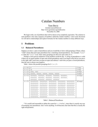
1. Catalan Numbers
Tom Davis
tomrdavis@earthlink.net
http://www.geometer.org/mathcircles
November 26, 2006
We begin with a set of problems that will be shown to be completely equivalent. The solution to
each problem is the same sequence of numbers called the Catalan numbers. Later in the document
we will derive relationships and explicit formulas for the Catalan numbers in many different ways.
1 Problems
1.1 Balanced Parentheses
Suppose you have n pairs of parentheses and you would like to form valid groupings of them, where
“valid” means that each open parenthesis has a matching closed parenthesis. For example, “(()())”
is valid, but “())()(” is not. How many groupings are there for each value of n?
Perhaps a more precise definition of the problem would be this: A string of parentheses is valid
if there are an equal number of open and closed parentheses and if you begin at the left as you move
to the right, add 1 each time you pass an open and subtract 1 each time you pass a closed parenthesis,
then the sum is always non-negative.
Table 1 shows the possible groupings for 0 ≤ n ≤ 5.
n = 0: * 1 way
n = 1: () 1 way
n = 2: ()(), (()) 2 ways
n = 3: ()()(), ()(()), (())(), (()()), ((())) 5 ways
n = 4: ()()()(), ()()(()), ()(())(), ()(()()), ()((())), 14 ways
(())()(), (())(()), (()())(), ((()))(), (()()()),
(()(())), ((())()), ((()())), (((())))
n = 5: ()()()()(), ()()()(()), ()()(())(), ()()(()()), ()()((())), 42 ways
()(())()(), ()(())(()), ()(()())(), ()((()))(), ()(()()()),
()(()(())), ()((())()), ()((()())), ()(((()))), (())()()(),
(())()(()), (())(())(), (())(()()), (())((())), (()())()(),
(()())(()), ((()))()(), ((()))(()), (()()())(), (()(()))(),
((())())(), ((()()))(), (((())))(), (()()()()), (()()(())),
(()(())()), (()(()())), (()((()))), ((())()()), ((())(())),
((()())()), (((()))()), ((()()())), ((()(()))), (((())())),
(((()()))), ((((()))))
Table 1: Balanced Parentheses
* It is useful and reasonable to define the count for n = 0 to be 1, since there is exactly one way
of arranging zero parentheses: don’t write anything. It will become clear later that this is exactly the
right interpretation.
1
2. 1.2 Mountain Ranges
How many “mountain ranges” can you form with n upstrokes and n downstrokes that all stay above
the original line? If, as in the case above, we consider there to be a single mountain range with zero
strokes, Table 2 gives a list of the possibilities for 0 ≤ n ≤ 3:
n = 0: * 1 way
n = 1: / 1 way
n = 2: / 2 ways
//, /
n = 3: / 5 ways
/ / // /
///, // , / /, / , /
Table 2: Mountain Ranges
Note that these must match the parenthesis-groupings above. The “(” corresponds to “/” and
the “) to “”. The mountain ranges for n = 4 and n = 5 have been omitted to save space, but there
are 14 and 42 of them, respectively. It is a good exercise to draw the 14 versions with n = 4.
In our formal definition of a valid set of parentheses, we stated that if you add one for open
parentheses and subtract one for closed parentheses that the sum would always remain non-negative.
The mountain range interpretation is that the mountains will never go below the horizon.
1.3 Diagonal-Avoiding Paths
In a grid of n×n squares, how many paths are there of length 2n that lead from the upper left corner
to the lower right corner that do not touch the diagonal dotted line from upper left to lower right? In
other words, how many paths stay on or above the main diagonal?
/ //
/ /
Figure 1: Corresponding Path and Range
This is obviously the same question as in the example above, with the mountain ranges running
diagonally. In Figure 1 we can see how one such path corresponds to a mountain range.
Another equivalent statement for this problem is the following. Suppose two candidates for
election, A and B, each receive n votes. The votes are drawn out of the voting urn one after the
other. In how many ways can the votes be drawn such that candidate A is never behind candidate
B?
2
3. 1.4 Polygon Triangulation
If you count the number of ways to triangulate a regular polygon with n + 2 sides, you also obtain
the Catalan numbers. Figure 2 illustrates the triangulations for polygons having 3, 4, 5 and 6 sides.
Figure 2: Polygon Triangulations
As you can see, there are 1, 2, 5, and 14 ways to do this. The “2-sided polygon” can also be
triangulated in exactly 1 way, so the case where n = 0 also matches.
1.5 Hands Across a Table
If 2n people are seated around a circular table, in how many ways can all of them be simultaneously
shaking hands with another person at the table in such a way that none of the arms cross each other?
Figure 3 illustrates the arrangements for 2, 4, 6 and 8 people. Again, there are 1, 2, 5 and 14 ways
to do this.
Figure 3: Hands Across the Table
3
4. 1.6 Binary Trees
The Catalan numbers also count the number of rooted binary trees with n internal nodes. Illustrated
in Figure 4 are the trees corresponding to 0 ≤ n ≤ 3. There are 1, 1, 2, and 5 of them. Try to draw
the 14 trees with n = 4 internal nodes.
A rooted binary tree is an arrangement of points (nodes) and lines connecting them where there
is a special node (the root) and as you descend from the root, there are either two lines going down
or zero. Internal nodes are the ones that connect to two nodes below.
Figure 4: Binary Trees
1.7 Plane Rooted Trees
A plane rooted tree is just like the binary tree above, except that a node can have any number of
sub-nodes; not just two.
Figure 5 shows a list of the plane rooted trees with n edges, for 0 ≤ n ≤ 3. Try to draw the 14
trees with n = 4 edges.
0 Edges:
1 Edge:
2 Edges:
3 Edges:
Figure 5: Plane Rooted Trees
1.8 Skew Polyominos
A polyomino is a set of squares connected by their edges. A skew polyomino is a polyomino such
that every vertical and horizontal line hits a connected set of squares and such that the successive
4
5. n = 1
n = 2
n = 3
n = 4
Table 3: Skew Polyominos with Perimeter 2n + 2
columns of squares from left to right increase in height—the bottom of the column to the left is
always lower or equal to the bottom of the column to the right. Similarly, the top of the column to
the left is always lower than or equal to the top of the column to the right. Table 3 shows a set of
such skew polyominos.
Another amazing result is that if you count the number of skew polyominos that have a perimeter
of 2n + 2, you will obtain Cn. Note that it is the perimeter that is fixed—not the number of squares
in the polyomino.
1.9 Multiplication Orderings
Suppose you have a set of n + 1 numbers to multiply together, meaning that there are n multipli-
cations to perform. Without changing the order of the numbers themselves, you can multiply the
numbers together in many orders. Here are the possible multiplication orderings for 0 ≤ n ≤ 4
multiplications. The groupings are indicated with parentheses and dot for multiplication in Table 4.
n = 0 (a) 1 way
n = 1 (a·b) 1 way
n = 2 ((a·b)·c), (a·(b·c)) 2 ways
n = 3 (((a·b)·c)·d), ((a·b)·(c·d)), ((a·(b·c))·d), 5 ways
(a·((b·c)·d)), (a·(b·(c·d)))
n = 4 ((((a·b)·c)·d)·e), (((a·b)·c)·(d·e)), (((a·b)·(c·d))·e), 14 ways
((a·b)·((c·d)·e)), ((a·b)·(c·(d·e))), (((a·(b·c))·d)·e),
((a·(b·c))·(d·e)), ((a·((b·c)·d))·e), ((a·(b·(c·d)))·e),
(a·(((b·c)·d)·e)), (a·((b·c)·(d·e))), (a·((b·(c·d))·e)),
(a·(b·((c·d)·e))), (a·(b·(c·(d·e))))
Table 4: Multiplication Arrangements
To convert the examples above to the parenthesis notation, erase everything but the dots and the
5
6. closed parentheses, and then replace the dots with open parentheses. For example, if we wish to
convert (a·(((b·c)·d)·e)), first erase everything but the dots and closed parentheses: ··)·)·)). Then
replace the dots with open parentheses to obtain: (()()()).
The examples in Table 4 are arranged in exactly the same order as the entries in Table 1 with the
correspondence described in the previous paragraph. Try to convert a few yourself in both directions
to make certain you understand the relationships.
2 A Recursive Definition
The examples above all seem to generate the same sequence of numbers. In fact it is obvious that
some are equivalent: parentheses, mountain ranges and diagonal-avoiding paths, for example. Later
on, we will prove that the other seqences are also the same. Once we’re convinced that they are the
same, we only need to have a formula that counts any one of them and the same formula will count
them all.
If you have no idea how to begin with a counting problem like this, one good approach is to write
down a formula that relates the count for a given n to previously-obtained counts. It is usually easy
to count the configurations for n = 0, n = 1, and n = 2 directly, and from there, you can count
more complex versions.
In this section, we’ll use the example with balanced parentheses discussed and illustrated in
Section 1.1. Let us assume that we already have the counts for 0, 1, 2, 3, · · ·, n − 1 pairs and we
would like to obtain the count for n pairs. Let Ci be the number of configurations of i matching
pairs of parentheses, so C0 = 1, C1 = 1, C2 = 2, C3 = 5, and C4 = 14, which can be obtained by
direct counts.
We know that in any balanced set, the first character has to be “(”. We also know that somewhere
in the set is the matching “)” for that opening one. In between that pair of parentheses is a balanced
set of parentheses, and to the right of it is another balanced set:
(A)B,
where A is a balanced set of parentheses and so is B. Both A and B can contain up to n − 1 pairs
of parentheses, but if A contains k pairs, then B contains n − k − 1 pairs. Notice that we will allow
either A or B to contain zero pairs, and that there is exactly one way to do so: don’t write down any
parentheses.
Thus we can count all the configurations where A has 0 pairs and B has n−1 pairs, where A has
1 pair and B has n − 2 pairs, and so on. Add them up, and we get the total number of configurations
with n balanced pairs.
Here are the formulas. It is a good idea to try plugging in the numbers you know to make certain
that you haven’t made a silly error. In this case, the formula for C3 indicates that it should be equal
to C3 = 2 · 1 + 1 · 1 + 1 · 2 = 5.
C1 = C0C0 (1)
C2 = C1C0 + C0C1 (2)
C3 = C2C0 + C1C1 + C0C2 (3)
C4 = C3C0 + C2C1 + C1C2 + C0C3 (4)
. . . . . .
6
7. Cn = Cn−1C0 + Cn−2C1 + · · · + C1Cn−2 + C0Cn−1 (5)
Beginning in the next section, we will be able to use these recursive formulas to show that the
counts of other configurations (triangulations of polygons, rooted binary trees, rooted tress, et cetera)
satisfy the same formulas and thus must generate the same sequence of numbers.
But simply by using the formulas above and a bit of arithmetic, it is easy to obtain the first
few Catalan numbers: 1, 1, 2, 5, 14, 42, 132, 429, 1430, 4862, 16796, 58786, 208012, 742900,
2674440, 9694845, 35357670, 129644790, 477638700, 1767263190, 6564120420, 24466267020,
91482563640, 343059613650, 1289904147324, . . .
2.1 Counting Polygon Triangulations
It is not hard to see that the polygon triangulations discussed in section 1.4 can be counted in much
the same way as the balanced parentheses. See Figure 6.
Figure 6: Octagon Triangulations
In the figure we consider the octagon, but it should be clear that the same argument applies to
any convex polygon. Consider the horizontal line at the top of the polygon. After triangulation, it
will be part of exactly one triangle, and in this case, there are exactly six possible triangles of which
it can be a part. In each case, once that triangle is selected, there is a polygon (possibly empty) on
the right and the left of the original triangle that must itself be triangulated.
What we would like to show is that a convex polygon with n > 3 sides can be triangulated in
Cn−2 ways. Thus the octagon should have C8−2 = C6 triangulations.
For the example in the upper left of Figure 6, the triangle leaves a 7-sided figure on the left and
an empty figure (essentially a two-sided polygon) on the right. This triangulation can be completed
by triangulating both sides; the one on the left can be done in C5 ways and the empty one on the
right, C0 ways, for a total of C5 ·C0. The middle example on the top leaves a pentagon and a triangle
that, in total, can be trianguated in C4 ·C1 ways. Similar arguments can be made for all six positions
of the triangle containing the top line, so we conclude that:
C6 = C5 · C0 + C4 · C1 + C3 · C2 + C2 · C3 + C1 · C4 + C0 · C5,
which is exactly how the Catalan numbers are defined for the nested parentheses.
Convince yourself that a similar argument can be made for any size original convex polygon.
7
8. 2.2 Counting Non-Crossing Handshakes
To count the number of hand-shakes discussed in Section 1.5 we can use an analysis similar to that
used in section 2.1.
If there are 2n people at the table pick any particular person, and that person will shake hands
with somebody. To admit a legal pattern, that person will have to leave an even number of people on
each side of the person with whom he shakes hands. Of the remaining n − 1 pairs of people, he can
leave zero on the right and n−1 pairs on the left, 1 on the right and n−2 on the left, and so on. The
pairs left on the right and left can independently choose any of the possible non-crossing handshake
patterns, so again, the count Cn for n pairs of people is given by:
Cn = Cn−1C0 + Cn−2C1 + · · · + C1Cn−2 + C0Cn−1,
which, together with the fact that C0 = C1 = 1, is just the definition of the Catalan numbers.
2.3 Counting Trees
Counting the binary trees discussed in Section 1.6 is similar to what we’ve done previously. Obvi-
ously there is one way to make a rooted binary tree with zero or one internal node. To work out the
number of trees with n internal node, note that one of those n nodes is the root node, and then the
n−1 additional internal nodes must be distributed on the left or the right below the root node. These
can be distributed as 0 on the left and n − 1 on the right, 1 on the left and n − 2 on the right, and so
on, yielding exactly the same formula that we had in every previous example.
To count the rooted plane trees discussed in Section 1.7 we use the same strategy. There is one
example each for trees with zero and one edge, so the counts here are the same: C0 = C1 = 1.
0 Edges:
1 Edge:
2 Edges:
3 Edges:
0×3:
1×2:
2×1:
3×0:
Figure 7: Plane Rooted Trees With 4 Edges
Now, to count the number of plane rooted trees with n > 1 edges we again begin from the root.
There is at least one edge going down (leaving us with n − 1 edges to draw). The remaining n − 1
edges can be placed below that initial edge or hooked directly to the root node to the right of that
8
9. edge. The n − 1 edges, as before, can be distributed to these two locations as 0 and n − 1, as 1 and
n − 2, et cetera. It should be clear that the same formula defining the Catalan numbers will apply to
the count of rooted plane trees.
In Figure 7 the table on the left dupliates the structure of trees with 3 or fewer edges and the table
on the right shows how the trees with 4 edges are generated from them.
2.4 Counting Diagonal-Avoiding Paths
Up to now we do not have an explicit formula for the Catalan numbers. We know that a large
collection of problems all have the same answers, and we have a recursive formula for those numbers,
but it would be nice to have an explicit form.
Perhaps the easiest way to obtain an explicit formula for the Catalan numbers is to analyze the
number of diagonal-avoiding paths discussed in Section 1.3. We will do so by counting the total
number of paths through the grid and then subtract off the number of paths that hit the diagonal.
:
P
:
P
Figure 8: Modifying a Bad Path
Figure 8 illustrates a typical path that we do not want to count since it crosses the dotted diagonal
line. Such a path may cross that line multiple times, but there is always a first time; in the figure,
point P is the first grid point it touches on the wrong side of the diagonal. There will always be such
a point P for every bad path.
For every such path, reflect the path beginning at P—every time the original path goes to the
right, go down instead, and when the original path goes down, go to the right. It is clear that by the
time the path reaches the point P it will have traveled one more step down than across, so it will
have moved k steps to the right and k + 1 steps down. The total path has n steps across and down,
so there remain n − k steps to the right and n − k − 1 steps down. But since we swap steps to the
right and steps down, the modified path with have a total of (k) + (n − k − 1) = n − 1 steps to the
right and (k + 1) + (n − k) = n + 1 steps down. Thus every modified path ends at the same point,
n − 1 steps to the right and n + 1 steps down.
Every bad path can be modified this way, and every path from the original starting point to this
point n − 1 to the right and n + 1 down corresponds to exactly one bad path. Thus the number of
bad paths is the total number of routes in a grid that is (n − 1) by (n + 1).
There are m+k
m paths through an k ×m grid1
. Thus the total number of paths through the n×n
grid is 2n
n and the total number of bad paths is 2n
n+1 . Thus Cn, the nth
Catalan number, or the
total number of diagonal-avoiding paths through an n × n grid, is given by:
Cn =
2n
n
−
2n
n + 1
=
2n
n
−
n
n + 1
2n
n
=
1
n + 1
2n
n
.
1To see this, remember that there are m steps down that need to be taken along the k +1 possible paths going down. Thus
the problem reduces to counting the number of ways of putting m objects in k + 1 boxes which is m+k
m
.
9
10. 3 Counting Mountain Ranges—Method 1
A very similar argument can be made as in the previous section if we use the interpretation of the
Catalan numbers based on the count of mountain ranges as described in Section 1.2. In that section,
we are seeking arrangements of n up-strokes and n down-strokes that form valid mountain ranges.
If we completely ignore whether the path is valid or not, we have n up-strokes that we can choose
from a collection of 2n available slots. In other words, ignoring path validity, we are simply asking
how many ways you can rearrange a collection of n up-strokes and n down-strokes. The answer is
clearly 2n
n .
Now we have to subtract off the bad paths. Every bad path goes below the horizon for the first
time at some point, so from that point on, reverse all the strokes—replace up-strokes with down-
strokes and vice-versa. It is clear that the new paths will all wind up 2 steps above the horizon, since
they consist of n + 1 up-strokes and n − 1 down-strokes. Conversely, every path that ends two steps
above the horizon must be of this form, so it corresponds to exactly one bad path.
How many such bad paths are there? The same number as there are ways to choose the n + 1
up-strokes from among the 2n total strokes, or 2n
n+1 .
Thus the count of valid mountain ranges, or Cn, is given by exactly the same formula:
Cn =
2n
n
−
2n
n + 1
=
2n
n
−
n
n + 1
2n
n
=
1
n + 1
2n
n
.
4 Counting Mountain Ranges—Method 2
Here is a different way to analyze the mountain problem. This time, imagine that we begin with
n + 1 up-strokes and only n down-strokes—we add an extra up-stroke to our collection.
First we solve the problem: How any arrangements can be made of these 2n + 1 symbols,
without worrying about whether they form a “valid” mountain range (whatever that means with an
unbalanced number of up-strokes and down-strokes). Clearly, if the ordering does not matter, there
are 2n+1
n ways to do this.
One thing is certain, however. No matter how they are arranged, they mountain range will be
one unit higher at the end, since we take n + 1 steps up and only n steps down.
Let’s look at a specific example with n = 3 (and 2n + 1 = 7): up up down up up down down.
In Figure 4, we have arranged this sequence over and over and you can see that every 7 steps, the
mountain range is one unit higher.
Figure 9: Growing Mountains
Since it is a repeating pattern, it’s clear that we can draw a straight line below it that touches the
bottom-most points of the growing mountain range.
10
11. In our example, this touching line seems to hit only once per complete set of 7 strokes, and we
will show that this will always be the case, for any unbalanced number of up-strokes and down-
strokes.
We can draw our mountain range on a grid, and it’s clear that the slope of the line is 1/(2n + 1)
(it goes up 1 unit in every complete cycle of the pattern of 2n + 1 strokes. But lines with slope
1/(2n + 1) can only hit lattice points every 2n + 1 units, so there is exactly one touching in each
complete cycle.
If you have a series of 2n + 1 strokes, you can cycle that around to 2n + 1 arrangements. For
example, the arrangement /// can be cycled to four other arrangements: ///, ///, ///
and ///. That means the complete set of arrangements can be divided into equivalence classes of
size 2n + 1, where two arrangements are equivalent if they are cycled versions of each other.
If we consider the version among these 2n + 1 cycles, the only one that yields a valid mountain
range is the one that begins at the low point of the 2n + 1 arrangement. Thus, to get a count of valid
mountain ranges with n up-strokes and n down-strokes, we need to divide our count of 2n+1 stroke
arrangements by 2n + 1:
Cn =
1
2n + 1
2n + 1
n
=
1
2n + 1
·
(2n + 1)!
n!(n + 1)!
=
1
n + 1
·
(2n)!
n! n!
=
1
n + 1
2n
n
.
Finally, note that when the line is drawn that touches the bottom edge of the range of mountains
with one more “up” than “down”, the first steps after the touching points are two “ups”, since an
“up-down” would immediately dip below the line. It should be clear that if one of the two initial
“up” moves is removed, the resulting series will stay above a horizontal line.
5 Generating Function Solution
Using the formulas 1 through 5 in Section 2, we can obtain an explicit formula for the Catalan
numbers, Cn using the technique known as generating functions.
We begin by defining a function f(z) that contains all of the Catalan numbers:
f(z) = C0 + C1z + C2z2
+ C3z3
+ · · · =
∞
i=0
Cizi
.
If we multiply f(z) by itself to obtain [f(z)]2
, the first few terms look like this:
[f(z)]2
= C0C0 + (C1C0 + C0C1)z + (C2C0 + C1C1 + C0C2)z2
+ · · · .
The coefficients for the powers of z are the same as those for the Catalan numbers obtained in
equations 1 through 5:
[f(z)]2
= C1 + C2z + C3z2
+ C4z3
+ · · · . (6)
We can convert Equation 6 back to f(z) if we multiply it by z and add C0, so we obtain:
f(z) = C0 + z[f(z)]2
. (7)
Equation 7 is just a quadratic equation in f(z) which we can solve using the quadratic formula.
In a more familiar form, we can rewrite it as: zf2
− f + C0 = 0. This is the same as the quadratic
11
12. equation: af2
+ bf + c = 0, where a = z, b = −1, and c = C0. Plug into the quadratic formula
and we obtain:
f(z) =
1 −
√
1 − 4z
2z
. (8)
Notice that we have used the − sign in place of the usual ± sign in the quadratic formula. We
know that f(0) = C0 = 1, so if we replaced the ± symbol with +, as z → 0, f(z) → ∞.
To expand f(z) we will just use the binomial formula on
√
1 − 4z = (1 − 4z)1/2
.
If you are not familiar with the use of the binomial formula with fractional exponents, don’t worry—
it is exactly the same, except that it never terminates.
Let’s look at the binomial formula for an integer exponent and just do the same calculation for a
fraction. If n is an integer, the binomial formula gives:
(a + b)n
= an
+
n
1
an−1
b1
+
n(n − 1)
2 · 1
an−2
b2
+
n(n − 1)(n − 2)
3 · 2 · 1
an−3
b3
+ · · · .
If n is an integer, eventually the numerator is going to have a term of the form (n − n), so that
term and all those beyond it will be zero. If n is not an integer, and it is 1/2 in our example, the
numerators will pass zero and continue. Here are the first few terms of the expansion of (1 −4z)1/2
:
(1 − 4z)1/2
= 1 −
1
2
1
4z +
1
2 − 1
2
2 · 1
(4z)2
−
1
2 − 1
2 − 3
2
3 · 2 · 1
(4z)3
+
1
2 − 1
2 − 3
2 − 5
2
4 · 3 · 2 · 1
(4z)4
−
1
2 − 1
2 − 3
2 − 5
2 − 7
2
5 · 4 · 3 · 2 · 1
(4z)5
+ · · ·
We can get rid of many powers of 2 and combine things to obtain:
(1 − 4z)1/2
= 1 −
1
1!
2z −
1
2!
4z2
−
3 · 1
3!
8z3
−
5 · 3 · 1
4!
16z4
−
7 · 5 · 3 · 1
5!
32z5
− · · · (9)
From Equations 9 and 8:
f(z) = 1 +
1
2!
2z +
3 · 1
3!
4z2
+
5 · 3 · 1
4!
8z3
+
7 · 5 · 3 · 1
5!
16z4
+ · · · (10)
The terms that look like 7 · 5 · 3 · 1 are a bit troublesome. They are like factorials, except they are
missing the even numbers. But notice that 22
·2! = 4·2, that 23
·3! = 6·4·2, that 24
·4! = 8·6·4·2,
et cetera. Thus (7 · 5 · 3 · 1) · 24
4! = 8!. If we apply this idea to Equation 10 we can obtain:
f(z) = 1 +
1
2
2!
1!1!
z +
1
3
4!
2!2!
z2
+
1
4
6!
3!3!
z3
+
1
5
8!
4!4!
z4
+ · · · =
∞
i=0
1
i + 1
2i
i
zi
.
From this we can conclude that the ith
Catalan number is given by the formula
Ci =
1
i + 1
2i
i
.
12