This document introduces the concept of a limit, which is the foundation of calculus. It provides an intuitive approach to understanding limits by examining how the instantaneous velocity of an object can be approximated by calculating average velocities over increasingly small time intervals. The key idea is that as the time intervals approach zero, the average velocities approach a limiting value that represents the instantaneous velocity. More generally, a limit describes how a function's values approach a specific number L as the input values approach a particular value a. The process of determining a limit involves first conjecturing the limit based on sampling function values, and then verifying it with a more rigorous analysis.
![January 10, 2001 13:09 g65-ch2 Sheet number 3 Page number 109 cyan magenta yellow black
2.1 Limits (An Intuitive Approach) 109
Table 2.1.1
0.5010
0.5005
0.5001
0.4999
0.4995
0.4990
12.9840
12.9920
12.9984
13.0016
13.0080
13.0160
vave(t1) =time t1 (s) (ft/s)
–16t1
2 + 29t1 – 10.5
t1 – 0.5
tions. It appears from these computations that a reasonable estimate for the instantaneous
velocity of the ball at time t = 0.5 s is 13 ft/s.
••
•
•
•
•
•
•
•
•
•
•
•
•
FOR THE READER. The domain of the height function s(t) = −16t2
+29t +6 in Example
1 is the closed interval [0, 2]. Why do we not consider values of t less than 0 or greater than
2 for this function? In Table 2.1.1, why is there not a value of vave(t1) for t1 = 0.5?
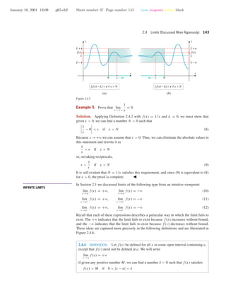
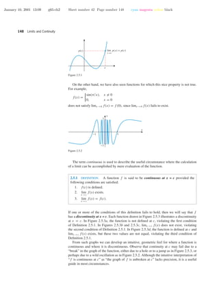
We can interpret vinst geometrically from the interpretation of vave as the slope of the
line joining the points (t0, s0) and (t1, s1) on the position versus time curve for the particle.
When t = t1 − t0 is small, the points (t0, s0) and (t1, s1) are very close to each other on
the curve. As the sampling point (t1, s1) is selected closer to our anchoring point (t0, s0),
the slope vave more nearly approximates what we might reasonably call the slope of the
position curve at time t = t0. Thus, vinst can be viewed as the slope of the position curve at
time t = t0 (Figure 2.1.3). We will explore this connection more fully in Section 3.1.
Slope = v ave
t0 t1
t
s
Slope=v
inst
Figure 2.1.3
• • • • • • • • • • • • • • • • • • • • • • • • • • • • • • • • • • • • • •
LIMITS
In Example 1 it appeared that choosing values of t1 close to (but not equal to) 0.5 resulted
in values of vave(t1) that were close to 13. One way of describing this behavior is to say that
the limiting value of vave(t1) as t1 approaches 0.5 is 13 or, equivalently, that 13 is the limit
of vave(t1) as t1 approaches 0.5. More generally, we will see that the concept of the limit of
a function provides a foundation for the tools of calculus. Thus, it is appropriate to start a
study of calculus by focusing on the limit concept itself.
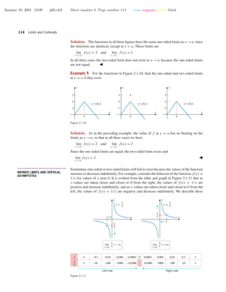
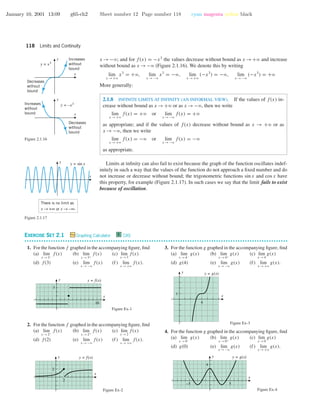
The most basic use of limits is to describe how a function behaves as the independent
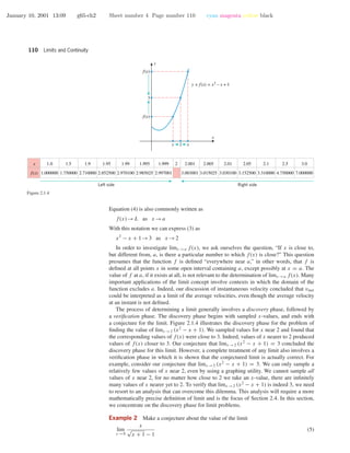
variable approaches a given value. For example, let us examine the behavior of the function
f(x) = x2
− x + 1
for x-values closer and closer to 2. It is evident from the graph and table in Figure 2.1.4 that
the values of f(x) get closer and closer to 3 as values of x are selected closer and closer
to 2 on either the left or the right side of 2. We describe this by saying that the “limit of
x2
− x + 1 is 3 as x approaches 2 from either side,” and we write
lim
x →2
(x2
− x + 1) = 3 (3)
Observe that in our investigation of limx →2 (x2
− x + 1) we are only concerned with the
values of f(x) near x = 2 and not the value of f(x) at x = 2.
This leads us to the following general idea.
2.1.1 LIMITS (AN INFORMAL VIEW). If the values of f(x) can be made as close as
we like to L by taking values of x sufficiently close to a (but not equal to a), then we
write
lim
x →a
f(x) = L (4)
which is read “the limit of f(x) as x approaches a is L.”](https://image.slidesharecdn.com/ch02-150306072941-conversion-gate01/85/Ch02-3-320.jpg)
![January 10, 2001 13:09 g65-ch2 Sheet number 14 Page number 120 cyan magenta yellow black
120 Limits and Continuity
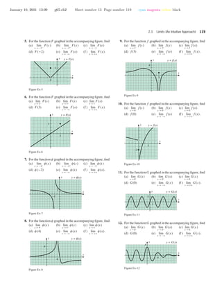
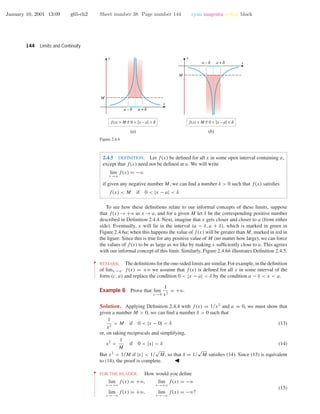
13. Consider the function g graphed in the accompanying fig-
ure. For what values of x0 does lim
x →x0
g(x) exist?
2–4
2
x
y y = g(x)
Figure Ex-13
14. Consider the function f graphed in the accompanying fig-
ure. For what values of x0 does lim
x →x0
f(x) exist?
3
4
x
y y = f(x)
Figure Ex-14
In Exercises 15–18, sketch a possible graph for a function f
with the specified properties. (Many different solutions are
possible.)
15. (i) f(0) = 2 and f(2) = 1
(ii) lim
x →1−
f(x) = +ϱ and lim
x →1+
f(x) = −ϱ
(iii) lim
x →+ϱ
f(x) = 0 and lim
x →−ϱ
f(x) = +ϱ
16. (i) f(0) = f(2) = 1
(ii) lim
x →2−
f(x) = +ϱ and lim
x →2+
f(x) = 0
(iii) lim
x →−1−
f(x) = −ϱ and lim
x →−1+
f(x) = +ϱ
(iv) lim
x →+ϱ
f(x) = 2 and lim
x →−ϱ
f(x) = +ϱ
17. (i) f(x) = 0 if x is an integer and f(x) = 0 if x is not an
integer
(ii) lim
x →+ϱ
f(x) = 0 and lim
x →−ϱ
f(x) = 0
18. (i) f(x) = 1 if x is a positive integer and f(x) = 1 if
x > 0 is not a positive integer
(ii) f(x) = −1 if x is a negative integer and f(x) = −1
if x < 0 is not a negative integer
(iii) lim
x →+ϱ
f(x) = 1 and lim
x →−ϱ
f(x) = −1
In Exercises 19–22: (i) Make a guess at the limit (if it ex-
ists) by evaluating the function at the specified x-values.
(ii) Confirm your conclusions about the limit by graphing
the function over an appropriate interval. (iii) If you have a
CAS, then use it to find the limit. [Note: For the trigonomet-
ric functions, be sure to set your calculating and graphing
utilities to the radian mode.]
C 19. (a) lim
x →1
x − 1
x3 − 1
; x = 2, 1.5, 1.1, 1.01, 1.001, 0, 0.5, 0.9,
0.99, 0.999
(b) lim
x →1+
x + 1
x3 − 1
; x = 2, 1.5, 1.1, 1.01, 1.001, 1.0001
(c) lim
x →1−
x + 1
x3 − 1
; x = 0, 0.5, 0.9, 0.99, 0.999, 0.9999
C 20. (a) lim
x →0
√
x + 1 − 1
x
; x = ±0.25, ±0.1, ±0.001,
±0.0001
(b) lim
x →0+
√
x + 1 + 1
x
; x = 0.25, 0.1, 0.001, 0.0001
(c) lim
x →0−
√
x + 1 + 1
x
; x = −0.25, −0.1, −0.001,
−0.0001
C 21. (a) lim
x →0
sin 3x
x
; x = ±0.25, ±0.1, ±0.001, ±0.0001
(b) lim
x →−1
cos x
x + 1
; x = 0, −0.5, −0.9, −0.99, −0.999,
−1.5, −1.1, −1.01, −1.001
C 22. (a) lim
x →−1
tan(x + 1)
x + 1
; x = 0, −0.5, −0.9, −0.99, −0.999,
−1.5, −1.1, −1.01, −1.001
(b) lim
x →0
sin(5x)
sin(2x)
; x = ±0.25, ±0.1, ±0.001, ±0.0001
23. Consider the motion of the ball described in Example 1. By
interpreting instantaneous velocity as a limit of average ve-
locity, make a conjecture for the value of the instantaneous
velocity of the ball 0.25 s after its release.
24. Consider the motion of the ball described in Example 1. By
interpreting instantaneous velocity as a limit of average ve-
locity, make a conjecture for the value of the instantaneous
velocity of the ball 0.75 s after its release.
In Exercises 25 and 26: (i) Approximate the y-coordinates
of all horizontal asymptotes of y = f(x) by evaluat-
ing f at the x-values ±10, ±100, ±1000, ±100,000, and
±100,000,000. (ii) Confirm your conclusions by graphing
y = f(x) over an appropriate interval. (iii) If you have a
CAS, then use it to find the horizontal asymptotes.
C 25. (a) f(x) =
2x + 3
x + 4
(b) f(x) = 1 +
3
x
x
(c) f(x) =
x2
+ 1
x + 1](https://image.slidesharecdn.com/ch02-150306072941-conversion-gate01/85/Ch02-14-320.jpg)
![January 10, 2001 13:09 g65-ch2 Sheet number 15 Page number 121 cyan magenta yellow black
2.1 Limits (An Intuitive Approach) 121
C 26. (a) f(x) =
x2
− 1
5x2 + 1
(b) f(x) = 2 +
1
x
x
(c) f(x) =
sin x
x
27. Assume that a particle is accelerated by a constant force.
The two curves v = n(t) and v = e(t) in the accompanying
figure provide velocity versus time curves for the particle
as predicted by classical physics and by the special theory
of relativity, respectively. The parameter c designates the
speed of light. Using the language of limits, describe the
differences in the long-term predictions of the two theories.
Time
v = n(t)
(Classical)
v = e(t)
(Relativity)
c
Velocity
v
t
Figure Ex-27
28. Let T = f(t) denote the temperature of a baked potato t
minutes after it has been removed from a hot oven. The ac-
companying figure shows the temperature versus time curve
for the potato, where r is the temperature of the room.
(a) What is the physical significance of lim
t →0+
f(t)?
(b) What is the physical significance of lim
t →+ϱ
f(t)?
Time (min)
T = f(t)
Temperature(°F)
T
t
400
r
Figure Ex-28
In Exercises 29 and 30: (i) Conjecture a limit from numerical
evidence. (ii) Use the substitution t = 1/x to express the
limit as an equivalent limit in which t → 0+
or t → 0−
, as
appropriate. (iii) Use a graphing utility to make a conjecture
about your limit in (ii).
29. (a) lim
x →+ϱ
x sin
1
x
(b) lim
x →+ϱ
1 − x
1 + x
(c) lim
x →−ϱ
1 +
2
x
x
30. (a) lim
x →+ϱ
cos(π/x)
π/x
(b) lim
x →+ϱ
x
1 + x
(c) lim
x →−ϱ
(1 − 2x)1/x
31. Suppose that f(x) denotes a function such that
lim
t →0
f(1/t) = L
What can be said about
lim
x →+ϱ
f(x) and lim
x →−ϱ
f(x)?
32. (a) Do any of the trigonometric functions, sin x, cos x,
tan x, cot x, sec x, csc x, have horizontal asymptotes?
(b) Do any of them have vertical asymptotes? Where?
33. (a) Let
f(x) = 1 + x2 1.1/x2
Graph f in the window [−1, 1]×[2.5, 3.5] and use the
calculator’s trace feature to make a conjecture about the
limit of f as x →0.
(b) Graph f in the window [−0.001, 0.001]×[2.5, 3.5] and
use the calculator’s trace feature to make a conjecture
about the limit of f as x →0.
(c) Graph f in the window [−0.000001, 0.000001] ×
[2.5, 3.5] and use the calculator’s trace feature to make
a conjecture about the limit of f as x →0.
(d) Later we will be able to show that
lim
x →0
1 + x2 1.1/x2
≈ 3.00416602
What flaw do your graphs reveal about using numerical
evidence (as revealed by the graphs you obtained) to
make conjectures about limits?
Roundoff error is one source of inaccuracy in calculator
and computer computations. Another source of error, called
catastrophicsubtraction,occurswhentwonearlyequalnum-
bers are subtracted, and the result is used as part of another
calculation. For example, by hand calculation we have
(0.123456789012345 − 0.123456789012344) × 1015
= 1
However, a calculator that can only store 14 decimal digits
produces a value of 0 for this computation, since the num-
bers being subtracted are identical in the first 14 digits. Catas-
trophic subtraction can sometimes be avoided by rearranging
formulas algebraically, but your best defense is to be aware
that it can occur. Watch out for it in the next exercise.
C 34. (a) Let
f(x) =
x − sin x
x3
Make a conjecture about the limit of f as x → 0+
by
evaluating f(x) at x = 0.1, 0.01, 0.001, 0.0001.
(b) Evaluate f(x) at x = 0.000001, 0.0000001,
0.00000001, 0.000000001, 0.0000000001, and make
another conjecture.
(c) What flaw does this reveal about using numerical evi-
dence to make conjectures about limits?
(d) If you have a CAS, use it to show that the exact value
of the limit is 1
6
.](https://image.slidesharecdn.com/ch02-150306072941-conversion-gate01/85/Ch02-15-320.jpg)
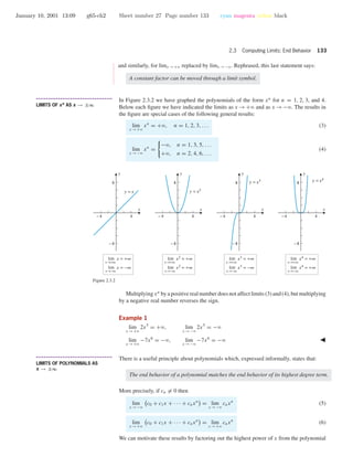
![January 10, 2001 13:09 g65-ch2 Sheet number 17 Page number 123 cyan magenta yellow black
2.2 Computing Limits 123
y = x
x a x
a
f(x) = x
f(x) = x
x
y
x
y
x
y
x
y
x a x
x →a
lim k = k
x →a
lim x = a
y = f(x) = k
k
x
y =
1
xy =
1
x
1
x
1
x
x
x→0+
lim = +∞
1
xx→0−
lim = −∞
1
x
Figure 2.2.1
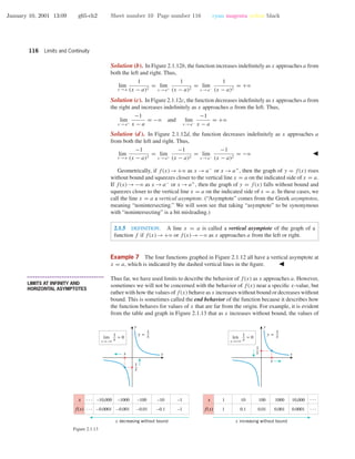
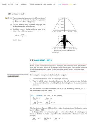
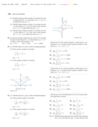
Since the identity function f(x) = x just echoes its input, it is clear that f(x) = x →a
as x →a. In terms of our informal definition of limits (2.1.1), if we decide just how close
to a we would like the value of f(x) = x to be, we need only restrict its input x to be just
as close to a.
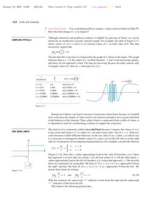
The one-sided limits of the reciprocal function f(x) = 1/x about 0 should conform
with your experience with fractions: making the denominator closer to zero increases the
magnitude of the fraction (i.e., increases its absolute value). This is illustrated in Table 2.2.1.
Table 2.2.1
values conclusion
–1
–1
1
1
x
1/x
x
1/x
–0.1
–10
0.1
10
– 0.01
–100
0.01
100
–0.001
–1000
0.001
1000
–0.0001
–10,000
0.0001
10,000
. . .
. . .
. . .
. . .
As x → 0–
the value of 1/x
decreases without bound.
As x → 0+
the value of 1/x
increases without bound.
The following theorem, parts of which are proved in Appendix G, will be our basic tool
for finding limits algebraically.
2.2.2 THEOREM. Let a be a real number, and suppose that
lim
x →a
f(x) = L1 and lim
x →a
g(x) = L2
That is, the limits exist and have values L1 and L2, respectively. Then,
(a) lim
x →a
[f(x) + g(x)] = lim
x →a
f(x) + lim
x →a
g(x) = L1 + L2
(b) lim
x →a
[f(x) − g(x)] = lim
x →a
f(x) − lim
x →a
g(x) = L1 − L2
(c) lim
x →a
[f(x)g(x)] = lim
x →a
f(x) lim
x →a
g(x) = L1L2
(d) lim
x →a
f(x)
g(x)
=
lim
x →a
f(x)
lim
x →a
g(x)
=
L1
L2
, provided L2 = 0
(e) lim
x →a
n
f(x) = n lim
x →a
f(x) = n
L1, provided L1 > 0 if n is even.
Moreover, these statements are also true for one-sided limits.](https://image.slidesharecdn.com/ch02-150306072941-conversion-gate01/85/Ch02-17-320.jpg)
![January 10, 2001 13:09 g65-ch2 Sheet number 18 Page number 124 cyan magenta yellow black
124 Limits and Continuity
A casual restatement of this theorem is as follows:
(a) The limit of a sum is the sum of the limits.
(b) The limit of a difference is the difference of the limits.
(c) The limit of a product is the product of the limits.
(d) The limit of a quotient is the quotient of the limits, provided the limit of the denom-
inator is not zero.
(e) The limit of an nth root is the nth root of the limit.
••
•
•
•
•
•
•
•
•
•
•
•
•
•
•
•
•
•
•
•
•
•
•
•
•
•
•
•
•
•
•
•
•
•
•
•
•
•
•
•
•
•
•
•
•
•
•
•
•
•
•
•
•
•
•
•
•
•
•
•
•
•
•
•
•
•
•
•
•
•
•
•
•
•
•
•
•
•
•
•
•
•
•
•
•
•
•
•
•
•
•
•
•
•
•
•
•
•
•
•
•
•
•
•
•
•
•
•
•
•
•
•
•
•
•
•
•
•
•
•
•
•
•
•
•
•
•
•
•
•
•
•
•
•
•
•
•
•
•
•
•
•
•
•
•
•
•
•
•
•
•
•
•
•
•
•
•
•
•
•
•
•
•
•
•
•
•
•
REMARK. Although results (a) and (c) in Theorem 2.2.2 are stated for two functions, they
hold for any finite number of functions. For example, if the limits of f(x), g(x), and h(x)
exist as x →a, then the limit of their sum and the limit of their product also exist as x →a
and are given by the formulas
lim
x →a
[f(x) + g(x) + h(x)] = lim
x →a
f(x) + lim
x →a
g(x) + lim
x →a
h(x)
lim
x →a
[f(x)g(x)h(x)] = lim
x →a
f(x) lim
x →a
g(x) lim
x →a
h(x)
In particular, if f(x) = g(x) = h(x), then this yields
lim
x →a
[f(x)]3
= lim
x →a
f(x)
3
More generally, if n is a positive integer, then the limit of the nth power of a function is the
nth power of the function’s limit. Thus,
lim
x →a
xn
= lim
x →a
x
n
= an
(1)
For example,
lim
x →3
x4
= 34
= 81
Another useful result follows from part (c) of Theorem 2.2.2 in the special case when
one of the factors is a constant k:
lim
x →a
(k · f(x)) = lim
x →a
k · lim
x →a
f(x) = k · lim
x →a
f(x) (2)
and similarly for limx →a replaced by a one-sided limit, limx →a+ or limx →a− . Rephrased,
this last statement says:
A constant factor can be moved through a limit symbol.
• • • • • • • • • • • • • • • • • • • • • • • • • • • • • • • • • • • • • •
LIMITS OF POLYNOMIALS AND
RATIONAL FUNCTIONS AS x → a
Example 1 Find lim
x →5
(x2
− 4x + 3) and justify each step.
Solution. First note that limx →5 x2
= 52
= 25 by Equation (1). Also, from Equation (2),
limx →5 4x = 4(limx →5 x) = 4(5) = 20. Since limx →5 3 = 3 by Theorem 2.2.1, we may
appeal to Theorem 2.2.2(a) and (b) to write
lim
x →5
(x2
− 4x + 3) = lim
x →5
x2
− lim
x →5
4x + lim
x →5
3 = 25 − 20 + 3 = 8
However, for conciseness, it is common to reverse the order of this argument and simply](https://image.slidesharecdn.com/ch02-150306072941-conversion-gate01/85/Ch02-18-320.jpg)
![January 10, 2001 13:09 g65-ch2 Sheet number 23 Page number 129 cyan magenta yellow black
2.2 Computing Limits 129
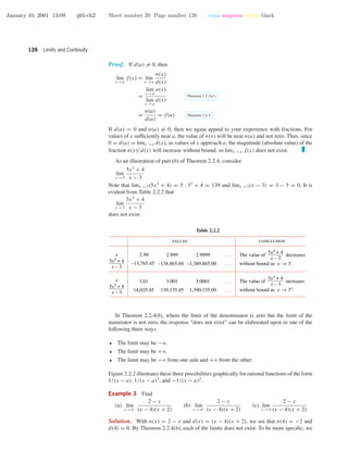
Solution (a). As x approaches −2 from the left, the formula for f is
f(x) =
1
x + 2
so that
lim
x →2−
f(x) = lim
x →2−
1
x + 2
= −ϱ
As x approaches −2 from the right, the formula for f is
f(x) = x2
− 5
so that
lim
x →−2+
f(x) = lim
x →2+
(x2
− 5) = (−2)2
− 5 = −1
Thus, limx →−2 f(x) does not exist.
Solution (b). As x approaches 0 from either the left or the right, the formula for f is
f(x) = x2
− 5
Thus,
lim
x →0
f(x) = lim
x →0
(x2
− 5) = 02
− 5 = −5
Solution (c). As x approaches 3 from the left, the formula for f is
f(x) = x2
− 5
so that
lim
x →3−
f(x) = lim
x →3−
(x2
− 5) = 32
− 5 = 4
As x approaches 3 from the right, the formula for f is
f(x) =
√
x + 13
so that
lim
x →3+
f(x) = lim
x →3+
√
x + 13 = lim
x →3+
(x + 13) =
√
3 + 13 = 4
Since the one-sided limits are equal, we have
lim
x →3
f(x) = 4
EXERCISE SET 2.2
• • • • • • • • • • • • • • • • • • • • • • • • • • • • • • • • • • • • • • • • • • • • • • • • • • • • • • • • • • • • • • • • • • • • • • • • • • • • • • • • • • • • • • • • • • • • • • • • • • • • • • • • • • • • • •
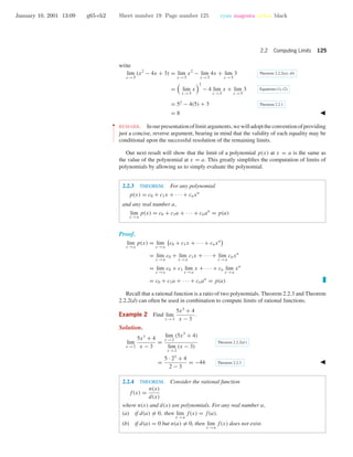
1. In each part, find the limit by inspection.
(a) lim
x →8
7 (b) lim
x →0+
π
(c) lim
x →−2
3x (d) lim
y →3+
12y
2. In each part, find the stated limit of f(x) = x/|x| by in-
spection.
(a) lim
x →5
f(x) (b) lim
x →−5
f(x)
(c) lim
x →0+
f(x) (d) lim
x →0−
f(x)
3. Given that
lim
x →a
f(x) = 2, lim
x →a
g(x) = −4, lim
x →a
h(x) = 0
find the limits that exist. If the limit does not exist, explain
why.
(a) lim
x →a
[f(x) + 2g(x)] (b) lim
x →a
[h(x) − 3g(x) + 1]
(c) lim
x →a
[f(x)g(x)] (d) lim
x →a
[g(x)]2
(e) lim
x →a
3
6 + f(x) (f) lim
x →a
2
g(x)
(g) lim
x →a
3f(x) − 8g(x)
h(x)
(h) lim
x →a
7g(x)
2f(x) + g(x)
4. Use the graphs of f and g in the accompanying figure to
find the limits that exist. If the limit does not exist, explain
why.](https://image.slidesharecdn.com/ch02-150306072941-conversion-gate01/85/Ch02-23-320.jpg)
![January 10, 2001 13:09 g65-ch2 Sheet number 24 Page number 130 cyan magenta yellow black
130 Limits and Continuity
(a) lim
x →2
[f(x) + g(x)] (b) lim
x →0
[f(x) + g(x)]
(c) lim
x →0+
[f(x) + g(x)] (d) lim
x →0−
[f(x) + g(x)]
(e) lim
x →2
f(x)
1 + g(x)
(f) lim
x →2
1 + g(x)
f(x)
(g) lim
x →0+
f(x) (h) lim
x →0−
f(x)
1
1
x
y
1
1
x
y
y = f(x) y = g(x)
Figure Ex-4
In Exercises 5–30, find the limits.
5. lim
y →2−
(y − 1)(y − 2)
y + 1
6. lim
x →3
x2
− 2x
x + 1
7. lim
x →4
x2
− 16
x − 4
8. lim
x →0
6x − 9
x3 − 12x + 3
9. lim
x →1+
x4
− 1
x − 1
10. lim
t →−2
t3
+ 8
t + 2
11. lim
x →−1
x2
+ 6x + 5
x2 − 3x − 4
12. lim
x →2
x2
− 4x + 4
x2 + x − 6
13. lim
t →2
t3
+ 3t2
− 12t + 4
t3 − 4t
14. lim
t →1
t3
+ t2
− 5t + 3
t3 − 3t + 2
15. lim
x →3+
x
x − 3
16. lim
x →3−
x
x − 3
17. lim
x →3
x
x − 3
18. lim
x →2+
x
x2 − 4
19. lim
x →2−
x
x2 − 4
20. lim
x →2
x
x2 − 4
21. lim
y →6+
y + 6
y2 − 36
22. lim
y →6−
y + 6
y2 − 36
23. lim
y →6
y + 6
y2 − 36
24. lim
x →4+
3 − x
x2 − 2x − 8
25. lim
x →4−
3 − x
x2 − 2x − 8
26. lim
x →4
3 − x
x2 − 2x − 8
27. lim
x →2+
1
|2 − x|
28. lim
x →3−
1
|x − 3|
29. lim
x →9
x − 9
√
x − 3
30. lim
y →4
4 − y
2 −
√
y
31. Verify the limit in Example 1 of Section 2.1. That is, find
lim
t1 →0.5
−16t2
1 + 29t1 − 10.5
t1 − 0.5
32. Let s(t) = −16t2
+ 29t + 6. Find
lim
t →1.5
s(t) − s(1.5)
t − 1.5
33. Let
f(x) =
x − 1, x ≤ 3
3x − 7, x > 3
Find
(a) lim
x →3−
f(x) (b) lim
x →3+
f(x) (c) lim
x →3
f(x).
34. Let
g(t) =
t2
, t ≥ 0
t − 2, t < 0
Find
(a) lim
t →0−
g(t) (b) lim
t →0+
g(t) (c) lim
t →0
g(t).
35. Let f(x) =
x3
− 1
x − 1
.
(a) Find lim
x →1
f(x).
(b) Sketch the graph of y = f(x).
36. Let
f(x) =
x2
− 9
x + 3
, x = −3
k, x = −3
(a) Find k so that f (−3) = lim
x →−3
f (x).
(b) With k assigned the value limx →−3 f (x), show that
f (x) can be expressed as a polynomial.
37. (a) Explain why the following calculation is incorrect.
lim
x →0+
1
x
−
1
x2
= lim
x →0+
1
x
− lim
x →0+
1
x2
= +ϱ − (+ϱ) = 0
(b) Show that lim
x →0+
1
x
−
1
x2
= −ϱ.
38. Find lim
x →0−
1
x
+
1
x2
.
In Exercises 39 and 40, first rationalize the numerator, then
find the limit.
39. lim
x →0
√
x + 4 − 2
x
40. lim
x →0
x2 + 4 − 2
x
41. Let p(x) and q(x) be polynomials, and suppose q(x0) = 0.
Discuss the behavior of the graph of y = p(x)/q(x) in the
vicinity of x = x0. Give examples to support your conclu-
sions.](https://image.slidesharecdn.com/ch02-150306072941-conversion-gate01/85/Ch02-24-320.jpg)
![January 10, 2001 13:09 g65-ch2 Sheet number 26 Page number 132 cyan magenta yellow black
132 Limits and Continuity
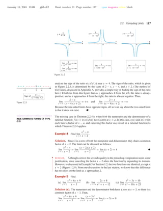
The limits of the reciprocal function f (x) = 1/x should make sense to you intuitively,
based on your experience with fractions: increasing the magnitude of x makes its reciprocal
closer to zero. This is illustrated in Table 2.3.1.
Table 2.3.1
values conclusion
–1
–1
1
1
x
1/x
x
1/x
–10
–0.1
10
0.1
–100
–0.01
100
0.01
–1000
–0.001
1000
0.001
–10,000
–0.0001
10,000
0.0001
. . .
. . .
. . .
. . .
As x → –∞ the value of 1/x
increases toward zero.
As x → +∞ the value of 1/x
decreases toward zero.
The following theorem mirrors Theorem 2.2.2 as our tool for finding limits at ±ϱ alge-
braically. (The proof is similar to that of the portions of Theorem 2.2.2 that are proved in
Appendix G.)
2.3.2 THEOREM. Suppose that
lim
x →+ϱ
f(x) = L1 and lim
x →+ϱ
g(x) = L2
That is, the limits exist and have values L1 and L2, respectively. Then,
(a) lim
x →+ϱ
[f(x) + g(x)] = lim
x →+ϱ
f(x) + lim
x →+ϱ
g(x) = L1 + L2
(b) lim
x →+ϱ
[f(x) − g(x)] = lim
x →+ϱ
f(x) − lim
x →+ϱ
g(x) = L1 − L2
(c) lim
x →+ϱ
[f(x)g(x)] = lim
x →+ϱ
f(x) lim
x →+ϱ
g(x) = L1L2
(d) lim
x →+ϱ
f(x)
g(x)
=
lim
x →+ϱ
f(x)
lim
x →+ϱ
g(x)
=
L1
L2
, provided L2 = 0
(e) lim
x →+ϱ
n
f(x) = n lim
x →+ϱ
f(x) = n
L1, provided L1 > 0 if n is even.
Moreover, these statements are also true if x →−ϱ.
••
•
•
•
•
•
•
•
•
•
•
•
•
•
•
•
•
•
•
•
•
•
•
•
•
•
•
•
•
•
•
•
•
•
•
•
•
•
•
•
•
•
•
•
•
•
•
•
•
•
•
•
•
•
•
•
•
•
•
•
•
•
•
•
•
•
•
•
•
•
•
•
•
•
•
•
•
•
•
•
•
•
•
•
•
•
•
•
•
•
•
•
•
REMARK. As in the remark following Theorem 2.2.2, results (a) and (c) can be extended to
sums or products of any finite number of functions. In particular, for any positive integer n,
lim
x →+ϱ
(f(x))n
= lim
x →+ϱ
f(x)
n
lim
x →−ϱ
(f(x))n
= lim
x →−ϱ
f(x)
n
Also, since limx →+ϱ(1/x) = 0, if n is a positive integer, then
lim
x →+ϱ
1
xn
= lim
x →+ϱ
1
x
n
= 0 lim
x →−ϱ
1
xn
= lim
x →−ϱ
1
x
n
= 0 (1)
For example,
lim
x →+ϱ
1
x4
= 0 and lim
x →−ϱ
1
x4
= 0
Another useful result follows from part (c) of Theorem 2.3.2 in the special case where
one of the factors is a constant k:
lim
x →+ϱ
(k · f(x)) = lim
x →+ϱ
k · lim
x →+ϱ
f(x) = k · lim
x →+ϱ
f(x) (2)](https://image.slidesharecdn.com/ch02-150306072941-conversion-gate01/85/Ch02-26-320.jpg)
![January 10, 2001 13:09 g65-ch2 Sheet number 30 Page number 136 cyan magenta yellow black
136 Limits and Continuity
1 and rationalize the numerator.
lim
x →+ϱ
( x6 + 5 − x3
) = lim
x →+ϱ
( x6 + 5 − x3
)
√
x6 + 5 + x3
√
x6 + 5 + x3
= lim
x →+ϱ
(x6
+ 5) − x6
√
x6 + 5 + x3
= lim
x →+ϱ
5
√
x6 + 5 + x3
= lim
x →+ϱ
5/x3
√
1 + 5/x6 + 1
√
x6 = x3
for x > 0
=
0
√
1 + 0 + 1
= 0
lim
x →+ϱ
( x6 + 5x3 − x3
) = lim
x →+ϱ
( x6 + 5x3 − x3
)
√
x6 + 5x3 + x3
√
x6 + 5x3 + x3
= lim
x →+ϱ
(x6
+ 5x3
) − x6
√
x6 + 5x3 + x3
= lim
x →+ϱ
5x3
√
x6 + 5x3 + x3
= lim
x →+ϱ
5
√
1 + 5/x3 + 1
√
x6 = x3
for x > 0
=
5
√
1 + 0 + 1
=
5
2
••
•
•
•
•
•
•
REMARK. Example 7 illustrates an indeterminate form of type ∞ – ∞. Exercises 31–34
explore more examples of this type.
EXERCISE SET 2.3 Graphing Calculator
• • • • • • • • • • • • • • • • • • • • • • • • • • • • • • • • • • • • • • • • • • • • • • • • • • • • • • • • • • • • • • • • • • • • • • • • • • • • • • • • • • • • • • • • • • • • • • • • • • • • • • • • • • • • • •
1. In each part, find the limit by inspection.
(a) lim
x →−ϱ
(−3) (b) lim
h→+ϱ
(−2h)
2. In each part, find the stated limit of f(x) = x/|x| by in-
spection.
(a) lim
x →+ϱ
f(x) (b) lim
x →−ϱ
f(x)
3. Given that
lim
x →+ϱ
f(x) = 3, lim
x →+ϱ
g(x) = −5, lim
x →+ϱ
h(x) = 0
find the limits that exist. If the limit does not exist, explain
why.
(a) lim
x →+ϱ
[f(x) + 3g(x)] (b) lim
x →+ϱ
[h(x) − 4g(x) + 1]
(c) lim
x →+ϱ
[f(x)g(x)] (d) lim
x →+ϱ
[g(x)]2
(e) lim
x →+ϱ
3
5 + f(x) (f) lim
x →+ϱ
3
g(x)
(g) lim
x →+ϱ
3h(x) + 4
x2
(h) lim
x →+ϱ
6f(x)
5f(x) + 3g(x)
4. Given that
lim
x →−ϱ
f(x) = 7, lim
x →−ϱ
g(x) = −6
find the limits that exist. If the limit does not exist, explain
why.
(a) lim
x →−ϱ
[2f(x) − g(x)] (b) lim
x →−ϱ
[6f(x) + 7g(x)]
(c) lim
x →−ϱ
[x2
+ g(x)] (d) lim
x →−ϱ
[x2
g(x)]
(e) lim
x →−ϱ
3
f(x)g(x) (f) lim
x →−ϱ
g(x)
f(x)
(g) lim
x →−ϱ
f(x) +
g(x)
x
(h) lim
x →−ϱ
xf(x)
(2x + 3)g(x)
In Exercises 5–28, find the limits.
5. lim
x →−ϱ
(3 − x) 6. lim
x →−ϱ
5 −
1
x
7. lim
x →+ϱ
(1 + 2x − 3x5
) 8. lim
x →+ϱ
(2x3
−100x+5)
9. lim
x →+ϱ
√
x 10. lim
x →−ϱ
√
5 − x
11. lim
x →+ϱ
3x + 1
2x − 5
12. lim
x →+ϱ
5x2
− 4x
2x2 + 3
13. lim
y →−ϱ
3
y + 4
14. lim
x →+ϱ
1
x − 12
15. lim
x →−ϱ
x − 2
x2 + 2x + 1
16. lim
x →+ϱ
5x2
+ 7
3x2 − x
17. lim
x →+ϱ
3 2 + 3x − 5x2
1 + 8x2
18. lim
s →+ϱ
3 3s7 − 4s5
2s7 + 1](https://image.slidesharecdn.com/ch02-150306072941-conversion-gate01/85/Ch02-30-320.jpg)
![January 10, 2001 13:09 g65-ch2 Sheet number 31 Page number 137 cyan magenta yellow black
2.3 Computing Limits: End Behavior 137
19. lim
x →−ϱ
5x2 − 2
x + 3
20. lim
x →+ϱ
5x2 − 2
x + 3
21. lim
y →−ϱ
2 − y
7 + 6y2
22. lim
y →+ϱ
2 − y
7 + 6y2
23. lim
x →−ϱ
3x4 + x
x2 − 8
24. lim
x →+ϱ
3x4 + x
x2 − 8
25. lim
x →+ϱ
7 − 6x5
x + 3
26. lim
t →−ϱ
5 − 2t3
t2 + 1
27. lim
t →+ϱ
6 − t3
7t3 + 3
28. lim
x →−ϱ
x + 4x3
1 − x2 + 7x3
29. Let
f(x) =
2x2
+ 5, x < 0
3 − 5x3
1 + 4x + x3
, x ≥ 0
Find
(a) lim
x →−ϱ
f(x) (b) lim
x →+ϱ
f(x).
30. Let
g(t) =
2 + 3t
5t2 + 6
, t < 1,000,000
√
36t2 − 100
5 − t
, t > 1,000,000
Find
(a) lim
t →−ϱ
g(t) (b) lim
t →+ϱ
g(t).
In Exercises 31–34, find the limits.
31. lim
x →+ϱ
( x2 + 3 − x) 32. lim
x →+ϱ
( x2 − 3x − x)
33. lim
x →+ϱ
( x2 + ax − x)
34. lim
x →+ϱ
( x2 + ax − x2 + bx)
35. Discuss the limits of p(x) = (1 − x)n
as x → +ϱ and
x →−ϱ for positive integer values of n.
36. Let p(x) = (1 − x)n
and q(x) = (1 − x)m
. Discuss the
limits of p(x)/q(x) as x → +ϱ and x → −ϱ for positive
integer values of m and n.
37. Let p(x) be a polynomial of degree n. Discuss the limits
of p(x)/xm
as x → +ϱ and x → −ϱ for positive integer
values of m.
38. In each part, find examples of polynomials p(x) and q(x)
that satisfy the stated condition and such that p(x) → +ϱ
and q(x)→+ϱ as x →+ϱ.
(a) lim
x →+ϱ
p(x)
q(x)
= 1 (b) lim
x →+ϱ
p(x)
q(x)
= 0
(c) lim
x →+ϱ
p(x)
q(x)
= +ϱ (d) lim
x →+ϱ
[p(x) − q(x)] = 3
39. Assuming that m and n are positive integers, find
lim
x →−ϱ
2 + 3xn
1 − xm
[Hint: Your answer will depend on whether m < n, m = n,
or m > n.]
40. Find
lim
x →+ϱ
c0 + c1x + · · · + cnxn
d0 + d1x + · · · + dmxm
where cn = 0 and dm = 0. [Hint: Your answer will depend
on whether m < n, m = n, or m > n.]
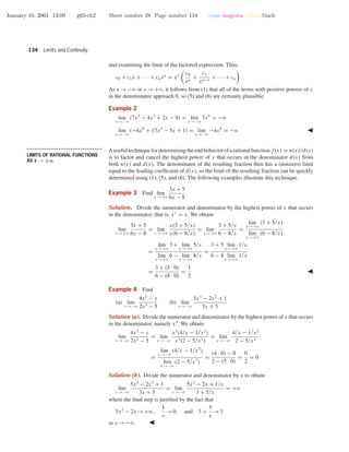
The notion of an asymptote can be extended to include curves
as well as lines. Specifically, we say that f(x) is asymptotic
to g(x) as x → +∞ if
lim
x →+ϱ
[f(x) − g(x)] = 0
and that f(x) is asymptotic to g(x) as x → –∞ if
lim
x →−ϱ
[f(x) − g(x)] = 0
Informally stated, if f(x) is asymptotic to g(x) as x →+ϱ,
then the graph of y = f(x) gets closer and closer to the graph
of y = g(x) as x →+ϱ, and if f(x) is asymptotic to g(x) as
x → −ϱ, then the graph of y = f(x) gets closer and closer
to the graph of y = g(x) as x →−ϱ. For example, if
f(x) = x2
+
2
x − 1
and g(x) = x2
then f(x) is asymptotic to g(x) as x →+ϱ and as x →−ϱ
since
lim
x →+ϱ
[f(x) − g(x)] = lim
x →+ϱ
1
x − 1
= 0
lim
x →−ϱ
[f(x) − g(x)] = lim
x →−ϱ
1
x − 1
= 0
This asymptotic behavior is illustrated in the following figure,
which also shows the vertical asymptote of f(x) at x = 1.
-4 -3 -2 -1 2 3 4
-10
-5
5
10
15
20
x
y
y = f(x)
y = g(x)
In Exercises 41–46, determine a function g(x) to which f(x)
is asymptotic as x →+ϱ or x →−ϱ. Use a graphing utility
to generate the graphs of y = f(x) and y = g(x) and identify
all vertical asymptotes.
41. f(x) =
x2
− 2
x − 2
42. f(x) =
x3
− x + 3
x
43. f(x) =
−x3
+ 3x2
+ x − 1
x − 3
44. f(x) =
x5
− x3
+ 3
x2 − 1
45. f(x) = sin x +
1
x − 1
46. f(x) =
x3 − x2 + 2
x − 1](https://image.slidesharecdn.com/ch02-150306072941-conversion-gate01/85/Ch02-31-320.jpg)
![January 10, 2001 13:09 g65-ch2 Sheet number 39 Page number 145 cyan magenta yellow black
2.4 Limits (Discussed More Rigorously) 145
EXERCISE SET 2.4 Graphing Calculator
• • • • • • • • • • • • • • • • • • • • • • • • • • • • • • • • • • • • • • • • • • • • • • • • • • • • • • • • • • • • • • • • • • • • • • • • • • • • • • • • • • • • • • • • • • • • • • • • • • • • • • • • • • • • • •
1. (a) Find the largest open interval, centered at the origin on
the x-axis, such that for each x in the interval the value
of the function f(x) = x + 2 is within 0.1 unit of the
number f(0) = 2.
(b) Find the largest open interval, centered at x = 3, such
that for each x in the interval the value of the func-
tion f(x) = 4x − 5 is within 0.01 unit of the number
f(3) = 7.
(c) Find the largest open interval, centered at x = 4, such
that for each x in the interval the value of the func-
tion f(x) = x2
is within 0.001 unit of the number
f(4) = 16.
2. In each part, find the largest open interval, centered at
x = 0, such that for each x in the interval the value of
f(x) = 2x + 3 is within units of the number f(0) = 3.
(a) = 0.1 (b) = 0.01
(c) = 0.0012
3. (a) Find the values of x1 and x2 in the accompanying figure.
(b) Find a positive number δ such that |
√
x − 2| < 0.05 if
0 < |x − 4| < δ.
4x1 x2
2 – 0.05
2 + 0.05
2
x
y
Not drawn to scale
y = √x
Figure Ex-3
4. (a) Find the values of x1 and x2 in the accompanying figure.
(b) Find a positive number δ such that |(1/x) − 1| < 0.1 if
0 < |x − 1| < δ.
1
1 – 0.1
1 + 0.1
1
x
y
x1
x2
Not drawn to scale
y =
1
x
Figure Ex-4
5. Generate the graph of f(x) = x3
− 4x + 5 with a graph-
ing utility, and use the graph to find a number δ such that
|f(x) − 2| < 0.05 if 0 < |x − 1| < δ. [Hint: Show
that the inequality |f(x) − 2| < 0.05 can be rewritten as
1.95 < x3
− 4x + 5 < 2.05, and estimate the values of x
for which x3
− 4x + 5 = 1.95 and x3
− 4x + 5 = 2.05.]
6. Use the method of Exercise 5 to find a number δ such that
|
√
5x + 1 − 4| < 0.5 if 0 < |x − 3| < δ.
7. Let f(x) = x +
√
x with L = limx →1 f(x) and let = 0.2.
Use a graphing utility and its trace feature to find a positive
number δ such that |f(x) − L| < if 0 < |x − 1| < δ.
8. Let f(x) = (sin 2x)/x and use a graphing utility to conjec-
ture the value of L = limx →0 f(x). Then let = 0.1 and
use the graphing utility and its trace feature to find a positive
number δ such that |f(x) − L| < if 0 < |x| < δ.
In Exercises 9–18, a positive number and the limit L of
a function f at a are given. Find a number δ such that
|f(x) − L| < if 0 < |x − a| < δ.
9. lim
x →4
2x = 8; = 0.1 10. lim
x →−2
1
2
x = −1; = 0.1
11. lim
x →−1
(7x + 5) = −2; = 0.01
12. lim
x →3
(5x − 2) = 13; = 0.01
13. lim
x →2
x2
− 4
x − 2
= 4; = 0.05
14. lim
x →−1
x2
− 1
x + 1
= −2; = 0.05
15. lim
x →4
x2
= 16; = 0.001 16. lim
x →9
√
x = 3; = 0.001
17. lim
x →5
1
x
=
1
5
; = 0.05 18. lim
x →0
|x| = 0; = 0.05
In Exercises 19–32, use Definition 2.4.1 to prove that the
stated limit is correct.
19. lim
x →5
3x = 15 20. lim
x →3
(4x − 5) = 7
21. lim
x →2
(2x − 7) = −3 22. lim
x →−1
(2 − 3x) = 5
23. lim
x →0
x2
+ x
x
= 1 24. lim
x →−3
x2
− 9
x + 3
= −6
25. lim
x →1
2x2
= 2 26. lim
x →3
(x2
− 5) = 4
27. lim
x →1/3
1
x
= 3 28. lim
x →−2
1
x + 1
= −1
29. lim
x →4
√
x = 2 30. lim
x →6
√
x + 3 = 3
31. lim
x →1
f(x) = 3, where f(x) =
x + 2, x = 1
10, x = 1
32. lim
x →2
(x2
+ 3x − 1) = 9
33. (a) Find the smallest positive number N such that for each
x in the interval (N, +ϱ), the value of the function
f(x) = 1/x2
is within 0.1 unit of L = 0.](https://image.slidesharecdn.com/ch02-150306072941-conversion-gate01/85/Ch02-39-320.jpg)
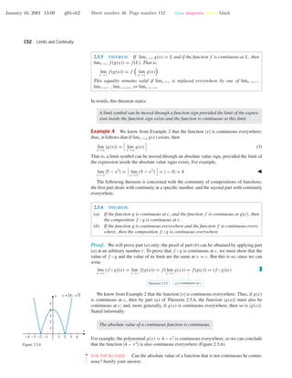
![January 10, 2001 13:09 g65-ch2 Sheet number 47 Page number 153 cyan magenta yellow black
2.5 Continuity 153
• • • • • • • • • • • • • • • • • • • • • • • • • • • • • • • • • • • • • •
CONTINUITY FROM THE LEFT
AND RIGHT
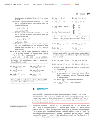
Because Definition 2.5.1 involves a two-sided limit, that definition does not generally apply
at the endpoints of a closed interval [a, b] or at the endpoint of an interval of the form
[a, b), (a, b], (−ϱ, b], or [a, +ϱ). To remedy this problem, we will agree that a function
is continuous at an endpoint of an interval if its value at the endpoint is equal to the appro-
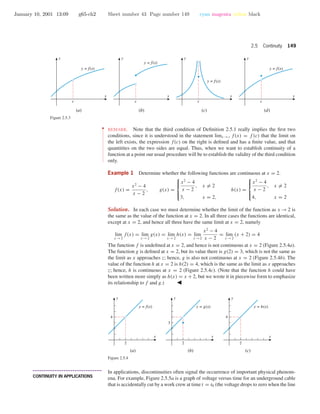
priate one-sided limit at that endpoint. For example, the function graphed in Figure 2.5.7 is
continuous at the right endpoint of the interval [a, b] because
lim
x →b−
f(x) = f(b)
but it is not continuous at the left endpoint because
lim
x →a+
f(x) = f(a)
In general, we will say a function f is continuous from the left at c if
lim
x →c−
f(x) = f(c)
and is continuous from the right at c if
lim
x →c+
f(x) = f(c)
Using this terminology we define continuity on a closed interval as follows.
x
y
y = f(x)
a b
Figure 2.5.7
2.5.7 DEFINITION. A function f is said to be continuous on a closed interval [a, b]
if the following conditions are satisfied:
1. f is continuous on (a, b).
2. f is continuous from the right at a.
3. f is continuous from the left at b.
••
•
•
•
•
•
•
FOR THE READER. We leave it for you to modify this definition appropriately so that it
applies to intervals of the form [a, +ϱ), (−ϱ, b], (a, b], and [a, b).
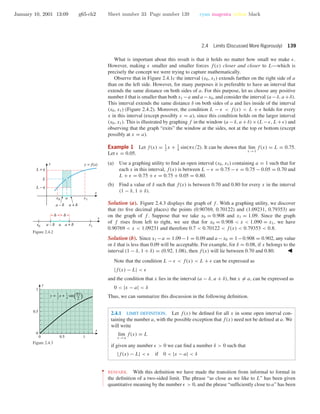
Example 5 What can you say about the continuity of the function f(x) = 9 − x2?
Solution. Because the natural domain of this function is the closed interval [−3, 3], we
will need to investigate the continuity of f on the open interval (−3, 3) and at the two
endpoints. If c is any number in the interval (−3, 3), then it follows from Theorem 2.2.2(e)
that
lim
x →c
f(x) = lim
x →c
9 − x2 = lim
x →c
(9 − x2) = 9 − c2 = f(c)
which proves f is continuous at each number in the interval (−3, 3). The function f is also
continuous at the endpoints since
lim
x →3−
f(x) = lim
x →3−
9 − x2 = lim
x →3−
(9 − x2) = 0 = f(3)
lim
x →−3+
f(x) = lim
x →−3+
9 − x2 = lim
x →−3+
(9 − x2) = 0 = f(−3)
Thus, f is continuous on the closed interval [−3, 3].
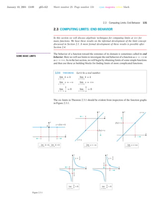
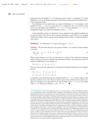
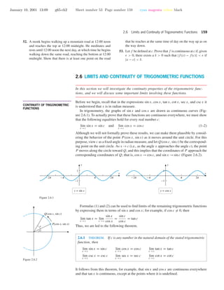
• • • • • • • • • • • • • • • • • • • • • • • • • • • • • • • • • • • • • •
THE INTERMEDIATE-VALUE
THEOREM
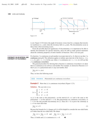
Figure 2.5.8 shows the graph of a function that is continuous on the closed interval [a, b].
The figure suggests that if we draw any horizontal line y = k, where k is between f(a)
and f(b), then that line will cross the curve y = f(x) at least once over the interval [a, b].
Stated in numerical terms, if f is continuous on [a, b], then the function f must take on
every value k between f(a) and f(b) at least once as x varies from a to b. For example,
the polynomial p(x) = x5
− x + 3 has a value of 3 at x = 1 and a value of 33 at x = 2.
Thus, it follows from the continuity of p that the equation x5
− x + 3 = k has at least one](https://image.slidesharecdn.com/ch02-150306072941-conversion-gate01/85/Ch02-47-320.jpg)
![January 10, 2001 13:09 g65-ch2 Sheet number 48 Page number 154 cyan magenta yellow black
154 Limits and Continuity
solution in the interval [1, 2] for every value of k between 3 and 33. This idea is stated more
precisely in the following theorem.
2.5.8 THEOREM (Intermediate-Value Theorem). If f is continuous on a closed interval
[a, b] and k is any number between f(a) and f(b), inclusive, then there is at least one
number x in the interval [a, b] such that f(x) = k.
x
y
f(a)
k
f(b)
a bx
Figure 2.5.8
Although this theorem is intuitively obvious, its proof depends on a mathematically precise
development of the real number system, which is beyond the scope of this text.
• • • • • • • • • • • • • • • • • • • • • • • • • • • • • • • • • • • • • •
APPROXIMATING ROOTS USING
THE INTERMEDIATE-VALUE
THEOREM
A variety of problems can be reduced to solving an equation f(x) = 0 for its roots. Some-
times it is possible to solve for the roots exactly using algebra, but often this is not possible
and one must settle for decimal approximations of the roots. One procedure for approxi-
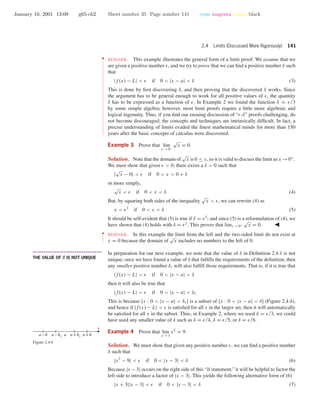
mating roots is based on the following consequence of the Intermediate-Value Theorem.
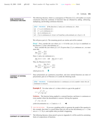
2.5.9 THEOREM. If f is continuous on [a, b], and if f(a) and f(b) are nonzero and
have opposite signs, then there is at least one solution of the equation f(x) = 0 in the
interval (a, b).
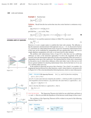
This result, which is illustrated in Figure 2.5.9, can be proved as follows.
x
y
f(a) > 0
f(b) < 0
f(x) = 0
a
b
Figure 2.5.9
Proof. Since f(a) and f(b) have opposite signs, 0 is between f(a) and f(b). Thus, by
the Intermediate-Value Theorem there is at least one number x in the interval [a, b] such
that f(x) = 0. However, f(a) and f(b) are nonzero, so x must lie in the interval (a, b),
which completes the proof.
Before we illustrate how this theorem can be used to approximate roots, it will be helpful
to discuss some standard terminology for describing errors in approximations. If x is an
approximation to a quantity x0, then we call
= |x − x0|
the absolute error or (less precisely) the error in the approximation. The terminology in
Table 2.5.1 is used to describe the size of such errors:
Table 2.5.1
error description
|x – x0| ≤ 0.1
|x – x0| ≤ 0.01
|x – x0| ≤ 0.001
|x – x0| ≤ 0.0001
|x – x0| ≤ 0.5
|x – x0| ≤ 0.05
|x – x0| ≤ 0.005
|x – x0| ≤ 0.0005
x approximates x0 with an error of at most 0.1.
x approximates x0 with an error of at most 0.01.
x approximates x0 with an error of at most 0.001.
x approximates x0 with an error of at most 0.0001.
x approximates x0 to the nearest integer.
x approximates x0 to 1 decimal place (i.e., to the nearest tenth).
x approximates x0 to 2 decimal places (i.e., to the nearest hundredth).
x approximates x0 to 3 decimal places (i.e., to the nearest thousandth).
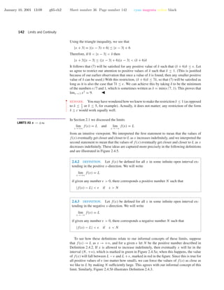
Example 6 The equation
x3
− x − 1 = 0
cannot be solved algebraically very easily because the left side has no simple factors.
However, if we graph p(x) = x3
− x − 1 with a graphing utility (Figure 2.5.10), then we
are led to conjecture that there is one real root and that this root lies inside the interval [1, 2].](https://image.slidesharecdn.com/ch02-150306072941-conversion-gate01/85/Ch02-48-320.jpg)
![January 10, 2001 13:09 g65-ch2 Sheet number 49 Page number 155 cyan magenta yellow black
2.5 Continuity 155
The existence of a root in this interval is also confirmed by Theorem 2.5.9, since p(1) = −1
and p(2) = 5 have opposite signs. Approximate this root to two decimal-place accuracy.
x
y
y = x3
– x – 1
2
2
Figure 2.5.10
Solution. Our objective is to approximate the unknown root x0 with an error of at most
0.005. It follows that if we can find an interval of length 0.01 that contains the root, then the
midpoint of that interval will approximate the root with an error of at most 0.01/2 = 0.005,
which will achieve the desired accuracy.
We know that the root x0 lies in the interval [1, 2]. However, this interval has length
1, which is too large. We can pinpoint the location of the root more precisely by dividing
the interval [1, 2] into 10 equal parts and evaluating p at the points of subdivision using
a calculating utility (Table 2.5.2). In this table p(1.3) and p(1.4) have opposite signs, so
we know that the root lies in the interval [1.3, 1.4]. This interval has length 0.1, which is
still too large, so we repeat the process by dividing the interval [1.3, 1.4] into 10 parts and
evaluating p at the points of subdivision; this yields Table 2.5.3, which tells us that the root
is inside the interval [1.32, 1.33] (Figure 2.5.11). Since this interval has length 0.01, its
midpoint 1.325 will approximate the root with an error of at most 0.005. Thus, x0 ≈ 1.325
to two decimal-place accuracy.
Table 2.5.2
1
–1
1.1
–0.77
1.2
–0.47
1.3
–0.10 0.34
1.5
0.88
1.6
1.50
1.7
2.21
1.8
3.03
1.4x
f(x)
1.9
3.96
2
5
Table 2.5.3
1.3
–0.103
1.31
–0.062
1.32
–0.020
1.33
0.023 0.066
1.35
0.110
1.36
0.155
1.37
0.201
1.38
0.248
1.34x
f(x)
1.39
0.296
1.4
0.344
1.322 1.324 1.326 1.328 1.330
-0.02
-0.01
0.01
0.02
x
y
y = p(x) = x3
– x – 1
Figure 2.5.11
• • • • • • • • • • • • • • • • • • • • • • • • • • • • • • • • • • • • • •
APPROXIMATING ROOTS BY
ZOOMING WITH A GRAPHING
UTILITY
The method illustrated in Example 6 can also be implemented with a graphing utility as
follows.
Step 1. Figure 2.5.12a shows the graph of f in the window [−5, 5]×[−5, 5]
with xScl = 1 and yScl = 1. That graph places the root between
x = 1 and x = 2.
Step 2. Since we know that the root lies between x = 1 and x = 2, we will
zoom in by regraphing f over an x-interval that extends between
these values and in which xScl = 0.1. The y-interval and yScl are not
critical, as long as the y-interval extends above and below the x-axis.
Figure 2.5.12b shows the graph of f in the window [1, 2] × [−1, 1]
with xScl = 0.1 and yScl = 0.1. That graph places the root between
x = 1.3 and x = 1.4.](https://image.slidesharecdn.com/ch02-150306072941-conversion-gate01/85/Ch02-49-320.jpg)
![January 10, 2001 13:09 g65-ch2 Sheet number 50 Page number 156 cyan magenta yellow black
156 Limits and Continuity
Step 3. Since we know that the root lies between x = 1.3 and x = 1.4, we
will zoom in again by regraphing f over an x-interval that extends
betweenthesevaluesandinwhichxScl = 0.01.Figure2.5.12cshows
the graph of f in the window [1.3, 1.4] × [−0.1, 0.1] with xScl =
0.01 and yScl = 0.01. That graph places the root between x = 1.32
and x = 1.33.
Step 4. Since the interval in Step 3 has length 0.01, its midpoint 1.325 ap-
proximates the root with an error of at most 0.005, so x0 ≈ 1.325 to
two decimal-place accuracy.
Figure 2.5.12
[–5, 5] × [–5, 5]
xScl = 1, yScl = 1
[1, 2] × [–1, 1]
xScl = 0.1, yScl = 0.1
[1.3, 1.4] × [–0.1, 0.1]
xScl = 0.01, yScl = 0.01
(b) (c)(a)
••
•
•
•
•
•
•
•
•
•
•
•
•
•
•
•
•
•
•
•
•
•
•
•
•
•
•
•
•
•
•
•
•
REMARK. To say that x approximates x0 to n decimal places does not mean that the first
n decimal places of x and x0 will be the same when the numbers are rounded to n decimal
places. For example, x = 1.084 approximates x0 = 1.087 to two decimal places because
|x − x0| = 0.003(<0.005). However, if we round these values to two decimal places, then
we obtain x ≈ 1.08 and x0 ≈ 1.09. Thus, if you approximate a number to n decimal places,
then you should display that approximation to at least n + 1 decimal places to preserve the
accuracy.
••
•
•
•
•
•
•
FOR THE READER. Use a graphing or calculating utility to show that the root x0 in Example
6 can be approximated as x0 ≈ 1.3245 to three decimal-place accuracy.
EXERCISE SET 2.5 Graphing Calculator
• • • • • • • • • • • • • • • • • • • • • • • • • • • • • • • • • • • • • • • • • • • • • • • • • • • • • • • • • • • • • • • • • • • • • • • • • • • • • • • • • • • • • • • • • • • • • • • • • • • • • • • • • • • • • •
In Exercises 1–4, let f be the function whose graph is shown.
On which of the following intervals, if any, is f continuous?
(a) [1, 3] (b) (1, 3) (c) [1, 2]
(d) (1, 2) (e) [2, 3] (f) (2, 3)
Foreachintervalonwhichf isnotcontinuous,indicatewhich
conditions for the continuity of f do not hold.
1.
1 2 3
x
y
2.
1 2 3
x
y
3.
1 2 3
x
y 4.
1 2 3
x
y
In Exercises 5 and 6, find all values of c such that the specified
function has a discontinuity at x = c. For each such value of
c, determine which conditions of Definition 2.5.1 fail to be
satisfied.](https://image.slidesharecdn.com/ch02-150306072941-conversion-gate01/85/Ch02-50-320.jpg)
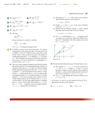
![January 10, 2001 13:09 g65-ch2 Sheet number 51 Page number 157 cyan magenta yellow black
2.5 Continuity 157
5. (a) The function f in Exercise 1 of Section 2.1.
(b) The function F in Exercise 5 of Section 2.1.
(c) The function f in Exercise 9 of Section 2.1.
6. (a) The function f in Exercise 2 of Section 2.1.
(b) The function F in Exercise 6 of Section 2.1.
(c) The function f in Exercise 10 of Section 2.1.
7. Suppose that f and g are continuous functions such that
f(2) = 1 and lim
x →2
[f(x) + 4g(x)] = 13. Find
(a) g(2) (b) lim
x →2
g(x).
8. Suppose that f and g are continuous functions such that
lim
x →3
g(x) = 5 and f(3) = −2. Find lim
x →3
[f(x)/g(x)].
9. In each part sketch the graph of a function f that satisfies
the stated conditions.
(a) f is continuous everywhere except at x = 3, at which
point it is continuous from the right.
(b) f has a two-sided limit at x = 3, but it is not continuous
at x = 3.
(c) f is not continuous at x = 3, but if its value at x = 3
is changed from f(3) = 1 to f(3) = 0, it becomes
continuous at x = 3.
(d) f is continuous on the interval [0, 3) and is defined on
the closed interval [0, 3]; but f is not continuous on the
interval [0, 3].
10. Find formulas for some functions that are continuous on the
intervals (−ϱ, 0) and (0, +ϱ), but are not continuous on the
interval (−ϱ, +ϱ).
11. A student parking lot at a university charges $2.00 for the
first half hour (or any part) and $1.00 for each subsequent
half hour (or any part) up to a daily maximum of $10.00.
(a) Sketch a graph of cost as a function of the time parked.
(b) Discuss the significance of the discontinuities in the
graph to a student who parks there.
12. In each part determine whether the function is continuous
or not, and explain your reasoning.
(a) The Earth’s population as a function of time
(b) Your exact height as a function of time
(c) The cost of a taxi ride in your city as a function of the
distance traveled
(d) The volume of a melting ice cube as a function of time
In Exercises 13–24, find the values of x (if any) at which f
is not continuous.
13. f(x) = x3
− 2x + 3 14. f(x) = (x − 5)17
15. f(x) =
x
x2 + 1
16. f(x) =
x
x2 − 1
17. f(x) =
x − 4
x2 − 16
18. f(x) =
3x + 1
x2 + 7x − 2
19. f(x) =
x
|x| − 3
20. f(x) =
5
x
+
2x
x + 4
21. f(x) = |x3
− 2x2
| 22. f(x) =
x + 3
|x2 + 3x|
23. f(x) =
2x + 3, x ≤ 4
7 +
16
x
, x > 4
24. f(x) =
3
x − 1
, x = 1
3, x = 1
25. Find a value for the constant k, if possible, that will make
the function continuous everywhere.
(a) f(x) =
7x − 2, x ≤ 1
kx2
, x > 1
(b) f(x) =
kx2
, x ≤ 2
2x + k, x > 2
26. On which of the following intervals is
f(x) =
1
√
x − 2
continuous?
(a) [2, +ϱ) (b) (−ϱ, +ϱ) (c) (2, +ϱ) (d) [1, 2)
A function f is said to have a removable discontinuity at
x = c if limx →c f(x) exists but f is not continuous at x = c,
either because f is not defined at c or because the definition
for f(c) differs from the value of the limit. This terminology
will be needed in Exercises 27–30.
27. (a) Sketch the graph of a function with a removable dis-
continuity at x = c for which f(c) is undefined.
(b) Sketch the graph of a function with a removable dis-
continuity at x = c for which f(c) is defined.
28. (a) The terminology removable discontinuity is appropri-
ate because a removable discontinuity of a function f
at x = c can be “removed” by redefining the value of
f appropriately at x = c. What value for f(c) removes
the discontinuity?
(b) Show that the following functions have removable dis-
continuities at x = 1, and sketch their graphs.
f(x) =
x2
− 1
x − 1
and g(x) =
1, x > 1
0, x = 1
1, x < 1
(c) What values should be assigned to f(1) and g(1) to
remove the discontinuities?
In Exercises 29 and 30, find the values of x (if any) at which
f is not continuous, and determine whether each such value
is a removable discontinuity.
29. (a) f(x) =
|x|
x
(b) f(x) =
x2
+ 3x
x + 3
(c) f(x) =
x − 2
|x| − 2](https://image.slidesharecdn.com/ch02-150306072941-conversion-gate01/85/Ch02-51-320.jpg)
![January 10, 2001 13:09 g65-ch2 Sheet number 52 Page number 158 cyan magenta yellow black
158 Limits and Continuity
30. (a) f(x) =
x2
− 4
x3 − 8
(b) f(x) =
2x − 3, x ≤ 2
x2
, x > 2
(c) f(x) =
3x2
+ 5, x = 1
6, x = 1
31. (a) Use a graphing utility to generate the graph of the func-
tion f(x) = (x + 3)/(2x2
+ 5x − 3), and then use
the graph to make a conjecture about the number and
locations of all discontinuities.
(b) Check your conjecture by factoring the denominator.
32. (a) Use a graphing utility to generate the graph of the func-
tion f(x) = x/(x3
− x + 2), and then use the graph to
make a conjecture about the number and locations of
all discontinuities.
(b) Use the Intermediate-Value Theorem to approximate
the location of all discontinuities to two decimal places.
33. Prove that f(x) = x3/5
is continuous everywhere, carefully
justifying each step.
34. Prove that f(x) = 1/ x4 + 7x2 + 1 is continuous every-
where, carefully justifying each step.
35. Let f and g be discontinuous at c. Give examples to show
that
(a) f + g can be continuous or discontinuous at c
(b) fg can be continuous or discontinuous at c.
36. Prove Theorem 2.5.4.
37. Prove:
(a) part (a) of Theorem 2.5.3
(b) part (b) of Theorem 2.5.3
(c) part (c) of Theorem 2.5.3.
38. Prove: If f and g are continuous on [a, b], and f(a) > g(a),
f(b) < g(b), then there is at least one solution of the equa-
tion f(x) = g(x) in (a, b). [Hint: Consider f(x) − g(x).]
39. Give an example of a function f that is defined on a closed
interval, and whose values at the endpoints have opposite
signs, but for which the equation f(x) = 0 has no solution
in the interval.
40. Use the Intermediate-Value Theorem to show that there is a
square with a diagonal length that is between r and 2r and
an area that is half the area of a circle of radius r.
41. Use the Intermediate-Value Theorem to show that there is
a right circular cylinder of height h and radius less than r
whose volume is equal to that of a right circular cone of
height h and radius r.
In Exercises 42 and 43, show that the equation has at least
one solution in the given interval.
42. x3
− 4x + 1 = 0; [1, 2] 43. x3
+x2
−2x = 1; [−1, 1]
44. Prove: If p(x) is a polynomial of odd degree, then the equa-
tion p(x) = 0 has at least one real solution.
45. The accompanying figure shows the graph of y = x4
+x−1.
Use the method of Example 6 to approximate the x-
intercepts with an error of at most 0.05.
[–5, 4] × [–3, 6]
xScl = 1, yScl = 1
Figure Ex-45
46. Use a graphing utility to solve the problem in Exercise 45
by zooming.
47. The accompanying figure shows the graph of y = 5−x−x4
.
Use the method of Example 6 to approximate the roots of
the equation 5−x −x4
= 0 to two decimal-place accuracy.
[–5, 4] × [–3, 6]
xScl = 1, yScl = 1
Figure Ex-47
48. Use a graphing utility to solve the problem in Exercise 47
by zooming.
49. Use the fact that
√
5 is a solution of x2
− 5 = 0 to approxi-
mate
√
5 with an error of at most 0.005.
50. Prove that if a and b are positive, then the equation
a
x − 1
+
b
x − 3
= 0
has at least one solution in the interval (1, 3).
51. A sphere of unknown radius x consists of a spherical core
and a coating that is 1 cm thick (see the accompanying fig-
ure). Given that the volume of the coating and the volume of
the core are the same, approximate the radius of the sphere
to three decimal-place accuracy.
1 cm
x
Figure Ex-51](https://image.slidesharecdn.com/ch02-150306072941-conversion-gate01/85/Ch02-52-320.jpg)
![January 10, 2001 13:09 g65-ch2 Sheet number 56 Page number 162 cyan magenta yellow black
162 Limits and Continuity
Solution (a).
lim
x →0
tan x
x
= lim
x →0
sin x
x
·
1
cos x
= (1)(1) = 1
Solution (b). The trick is to multiply and divide by 2, which will make the denominator
the same as the argument of the sine function [just as in Theorem 2.6.3(a)]:
lim
θ →0
sin 2θ
θ
= lim
θ →0
2 ·
sin 2θ
2θ
= 2 lim
θ →0
sin 2θ
2θ
Now make the substitution x = 2θ, and use the fact that x →0 as θ →0. This yields
lim
θ →0
sin 2θ
θ
= 2 lim
θ →0
sin 2θ
2θ
= 2 lim
x →0
sin x
x
= 2(1) = 2
Solution (c).
lim
x →0
sin 3x
sin 5x
= lim
x →0
sin 3x
x
sin 5x
x
= lim
x →0
3 ·
sin 3x
3x
5 ·
sin 5x
5x
=
3 · 1
5 · 1
=
3
5
••
•
•
•
•
•
•
•
FOR THE READER. Use a graphing utility to confirm the limits in the last example graph-
ically, and if you have a CAS, then use it to obtain the limits.
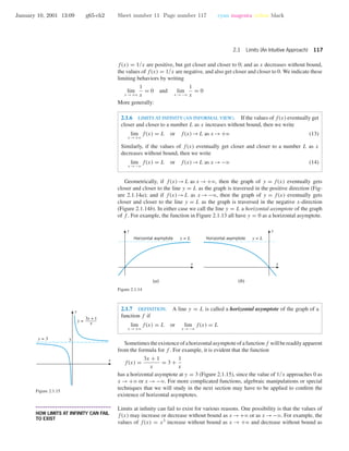
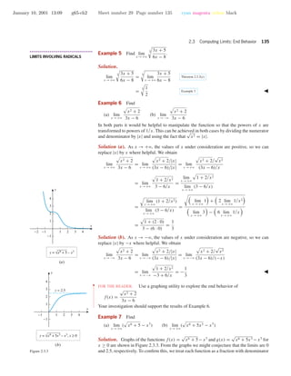
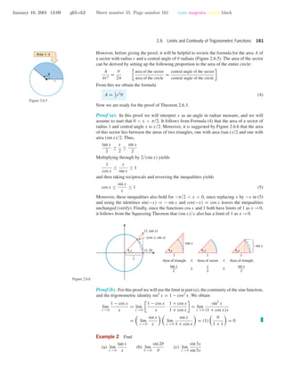
Example 3 Make conjectures about the limits
(a) lim
x →0
sin
1
x
(b) lim
x →0
x sin
1
x
and confirm your conclusions by generating the graphs of the functions near x = 0 using a
graphing utility.
Solution (a). Since 1/x → +ϱ as x → 0+
, we can view sin(1/x) as the sine of an angle
that increases indefinitely as x →0+
. As this angle increases, the function sin(1/x) keeps
oscillating between −1 and 1 without approaching a limit. Similarly, there is no limit from
the left since 1/x → −ϱ as x → 0−
. These conclusions are consistent with the graph of
y = sin(1/x) shown in Figure 2.6.7a. Observe that the oscillations become more and more
rapid as x approaches 0 because 1/x increases (or decreases) more and more rapidly as x
approaches 0.
Solution (b). If x > 0, −x ≤ x sin(1/x) ≤ x, and if x < 0, x ≤ x sin(1/x) ≤ −x.
Thus, for x = 0, −|x| ≤ x sin(1/x) ≤ |x|. Since both |x| → 0 and −|x| → 0 as x → 0,
the Squeezing Theorem applies and we can conclude that x sin(1/x)→0 as x →0. This is
illustrated in Figure 2.6.7b.
-1 1
-1
1
x
y
y = sin ( )x
1
(a)
y = x sin ( )x
1
x
y
y = |x|
y = –|x|
(b)
Figure 2.6.7
••
•
•
•
•
•
•
•
•
•
•
•
•
•
•
•
•
•
•
•
•
•
•
•
•
•
•
•
•
•
•
•
•
•
REMARK. It follows from part (b) of this example that the function
f(x) =
x sin(1/x), x = 0
0, x = 0
is continuous at x = 0, since the value of the function and the value of the limit are the
same at 0. This shows that the behavior of a function can be very complex in the vicinity
of an x-value c, even though the function is continuous at c.](https://image.slidesharecdn.com/ch02-150306072941-conversion-gate01/85/Ch02-56-320.jpg)
![January 10, 2001 13:09 g65-ch2 Sheet number 57 Page number 163 cyan magenta yellow black
2.6 Limits and Continuity of Trigonometric Functions 163
EXERCISE SET 2.6 Graphing Calculator C CAS
• • • • • • • • • • • • • • • • • • • • • • • • • • • • • • • • • • • • • • • • • • • • • • • • • • • • • • • • • • • • • • • • • • • • • • • • • • • • • • • • • • • • • • • • • • • • • • • • • • • • • • • • • • • • • •
In Exercises 1–10, find the discontinuities, if any.
1. f(x) = sin(x2
− 2) 2. f(x) = cos
x
x − π
3. f(x) = cot x 4. f(x) = sec x
5. f(x) = csc x 6. f(x) =
1
1 + sin2
x
7. f(x) = | cos x| 8. f(x) = 2 + tan2 x
9. f(x) =
1
1 − 2 sin x
10. f(x) =
3
5 + 2 cos x
11. Use Theorem 2.5.6 to show that the following functions
are continuous everywhere by expressing them as compo-
sitions of simpler functions that are known to be continuous.
(a) sin(x3
+ 7x + 1) (b) |sin x|
(c) cos3
(x + 1) (d)
√
3 + sin 2x
(e) sin(sin x) (f) cos5
x − 2 cos3
x + 1
12. (a) Prove that if g(x) is continuous everywhere, then so are
sin(g(x)), cos(g(x)), g(sin(x)), and g(cos(x)).
(b) Illustrate the result in part (a) with some of your own
choices for g.
Find the limits in Exercises 13–35.
13. lim
x →+ϱ
cos
1
x
14. lim
x →+ϱ
sin
2
x
15. lim
x →+ϱ
sin
πx
2 − 3x
16. lim
h→0
sin h
2h
17. lim
θ →0
sin 3θ
θ
18. lim
θ →0+
sin θ
θ2
19. lim
x →0−
sin x
|x|
20. lim
x →0
sin2
x
3x2
21. lim
x →0+
sin x
5
√
x
22. lim
x →0
sin 6x
sin 8x
23. lim
x →0
tan 7x
sin 3x
24. lim
θ →0
sin2
θ
θ
25. lim
h→0
h
tan h
26. lim
h→0
sin h
1 − cos h
27. lim
θ →0
θ2
1 − cos θ
28. lim
x →0
x
cos 1
2
π − x
29. lim
θ →0
θ
cos θ
30. lim
t →0
t2
1 − cos2 t
31. lim
h→0
1 − cos 5h
cos 7h − 1
32. lim
x →0+
sin
1
x
33. lim
x →0+
cos
1
x
34. lim
x →0
x2
− 3 sin x
x
35. lim
x →0
2x + sin x
x
In Exercises 36–39: (i) Construct a table to estimate the limit
by evaluating the function near the limiting value. (ii) Find
the exact value of the limit.
36. lim
x →5
sin(x − 5)
x2 − 25
37. lim
x →2
sin(2x − 4)
x2 − 4
38. lim
x →−2
sin(x2
+ 3x + 2)
x + 2
39. lim
x →−1
sin(x2
+ 3x + 2)
x3 + 1
40. Find a value for the constant k that makes
f(x) =
sin 3x
x
, x = 0
k, x = 0
continuous at x = 0.
41. Find a nonzero value for the constant k that makes
f(x) =
tan kx
x
, x < 0
3x + 2k2
, x ≥ 0
continuous at x = 0.
42. Is
f(x) =
sin x
|x|
, x = 0
1, x = 0
continuous at x = 0?
43. In each part, find the limit by making the indicated substi-
tution.
(a) lim
x →+ϱ
x sin
1
x
; t =
1
x
(b) lim
x →−ϱ
x 1 − cos
1
x
; t =
1
x
(c) lim
x →π
π − x
sin x
. [Hint: Let t = π − x.]
44. Find lim
x →2
cos(π/x)
x − 2
; t =
π
2
−
π
x
.
45. Find lim
x →1
sin(πx)
x − 1
. 46. Find lim
x →π/4
tan x−1
x−π/4
.
47. Use the Squeezing Theorem to show that
lim
x →0
x cos
50π
x
= 0
and illustrate the principle involved by using a graphing util-
ity to graph y = |x|, y = −|x|, and y = x cos(50π/x) on
the same screen in the window [−1, 1] × [−1, 1].
48. Use the Squeezing Theorem to show that
lim
x →0
x2
sin
50π
3
√
x
= 0](https://image.slidesharecdn.com/ch02-150306072941-conversion-gate01/85/Ch02-57-320.jpg)
![January 10, 2001 13:09 g65-ch2 Sheet number 58 Page number 164 cyan magenta yellow black
164 Limits and Continuity
and illustrate the principle involved by using a graphing util-
ity to graph y = x2
, y = −x2
, and y = x2
sin(50π/ 3
√
x ) on
the same screen in the window [−0.5, 0.5]×[−0.25, 0.25].
49. Sketch the graphs of y = 1 − x2
, y = cos x, and y = f(x),
where f is a function that satisfies the inequalities
1 − x2
≤ f(x) ≤ cos x
for all x in the interval (−π/2, π/2). What can you say about
the limit of f(x) as x →0? Explain your reasoning.
50. Sketch the graphs of y = 1/x, y = −1/x, and y = f(x),
where f is a function that satisfies the inequalities
−
1
x
≤ f(x) ≤
1
x
for all x in the interval [1, +ϱ). What can you say about the
limit of f(x) as x →+ϱ? Explain your reasoning.
51. Find formulas for functions g and h such that g(x)→0 and
h(x)→0 as x →+ϱ and such that
g(x) ≤
sin x
x
≤ h(x)
for positive values of x. What can you say about the limit
lim
x →+ϱ
sin x
x
?
Explain your reasoning.
52. Draw pictures analogous to Figure 2.6.3 that illustrate the
Squeezing Theorem for limits of the forms limx →+ϱ f(x)
and limx →−ϱ f(x).
Recall that unless stated otherwise the variable x in trigono-
metric functions such as sin x and cos x is assumed to be in
radian measure. The limits in Theorem 2.6.3 are based on
that assumption. Exercises 53 and 54 explore what happens
to those limits if degree measure is used for x.
53. (a) Show that if x is in degrees, then
lim
x →0
sin x
x
=
π
180
(b) Confirm that the limit in part (a) is consistent with the
results produced by your calculating utility by setting
the utility to degree measure and calculating (sin x)/x
for some values of x that get closer and closer to 0.
54. What is the limit of (1−cos x)/x as x →0 if x is in degrees?
55. It follows from part (a) of Theorem 2.6.3 that if θ is small
(near zero) and measured in radians, then one should expect
the approximation
sin θ ≈ θ
to be good.
(a) Find sin 10◦
using a calculating utility.
(b) Estimate sin 10◦
using the approximation above.
56. (a) Use the approximation of sin θ that is given in Exer-
cise 55 together with the identity cos 2α = 1 − 2 sin2
α
with α = θ/2 to show that if θ is small (near zero)
and measured in radians, then one should expect the
approximation
cos θ ≈ 1 − 1
2
θ2
to be good.
(b) Find cos 10◦
using a calculating utility.
(c) Estimate cos 10◦
using the approximation above.
57. It follows from part (a) of Example 2 that if θ is small (near
zero) and measured in radians, then one should expect the
approximation
tan θ ≈ θ
to be good.
(a) Find tan 5◦
using a calculating utility.
(b) Find tan 5◦
using the approximation above.
58. Referring to the accompanying figure, suppose that the an-
gle of elevation of the top of a building, as measured from
a point L feet from its base, is found to be α degrees.
(a) Use the relationship h = L tan α to calculate the height
of a building for which L = 500 ft and α = 6◦
.
(b) Show that if L is large compared to the building height
h, then one should expect good results in approximating
h by h ≈ πLα/180.
(c) Use the result in part (b) to approximate the building
height h in part (a).
ha
L Figure Ex-58
59. (a) Use the Intermediate-Value Theorem to show that the
equation x = cos x has at least one solution in the in-
terval [0, π/2].
(b) Show graphically that there is exactly one solution in
the interval.
(c) Approximate the solution to three decimal places.
60. (a) Use the Intermediate-Value Theorem to show that the
equation x + sin x = 1 has at least one solution in the
interval [0, π/6].
(b) Show graphically that there is exactly one solution in
the interval.
(c) Approximate the solution to three decimal places.
61. In the study of falling objects near the surface of the Earth,
the acceleration g due to gravity is commonly taken to be
9.8 m/s2
or 32 ft/s2
. However, the elliptical shape of the
Earth and other factors cause variations in this constant that
are latitude dependent. The following formula, known as the
Geodetic Reference Formula of 1967, is commonly used to
predict the value of g at a latitude of φ degrees (either north
or south of the equator):
g = 9.7803185(1.0 + 0.005278895 sin2
φ
− 0.000023462 sin4
φ) m/s2
(a) Observe that g is an even function of φ. What does this
suggest about the shape of the Earth, as modeled by the
Geodetic Reference Formula?](https://image.slidesharecdn.com/ch02-150306072941-conversion-gate01/85/Ch02-58-320.jpg)
![January 10, 2001 13:09 g65-ch2 Sheet number 59 Page number 165 cyan magenta yellow black
Supplementary Exercises 165
(b) Show that g = 9.8 m/s2
somewhere between latitudes
of 38◦
and 39◦
.
62. Let
f(x) =
1 if x is a rational number
0 if x is an irrational number
(a) Make a conjecture about the limit of f(x) as x →0.
(b) Make a conjecture about the limit of xf(x) as x →0.
(c) Prove your conjectures.
SUPPLEMENTARY EXERCISES
1. For the function f graphed in the accompanying figure, find
the limit if it exists.
(a) lim
x →1
f(x) (b) lim
x →2
f(x) (c) lim
x →3
f(x)
(d) lim
x →4
f(x) (e) lim
x →+ϱ
f(x) (f) lim
x →−ϱ
f(x)
(g) lim
x →3+
f(x) (h) lim
x →3−
f(x) (i) lim
x →0
f(x)
-1 1 2 3 4 5 6 7 8
1
2
3
x
y
Figure Ex-1
2. (a) Find a formula for a rational function that has a verti-
cal asymptote at x = 1 and a horizontal asymptote at
y = 2.
(b) Check your work by using a graphing utility to graph
the function.
3. (a) Write a paragraph or two that describes how the limit of
a function can fail to exist at x = a. Accompany your
description with some specific examples.
(b) Write a paragraph or two that describes how the limit
of a function can fail to exist as x → +ϱ or x → −ϱ.
Also, accompany your description with some specific
examples.
(c) Write a paragraph or two that describes how a function
can fail to be continuous at x = a. Accompany your
description with some specific examples.
4. Show that the conclusion of the Intermediate-Value The-
orem may be false if f is not continuous on the interval
[a, b].
5. In each part, evaluate the function for the stated values of x,
and make a conjecture about the value of the limit. Confirm
your conjecture by finding the limit algebraically.
(a) f(x) =
x − 2
x2 − 4
; lim
x →2+
f(x); x = 2.5, 2.1, 2.01,
2.001, 2.0001, 2.00001
(b) f(x) =
tan 4x
x
; lim
x →0
f(x); x = ±1.0, ±0.1, ±0.01,
±0.001, ±0.0001, ±0.00001
6. In each part, find the horizontal asymptotes, if any.
(a) y =
2x − 7
x2 − 4x
(b) y =
x3
− x2
+ 10
3x2 − 4x
(c) y =
2x2
− 6
x2 + 5x
7. (a) Approximate the value for the limit
lim
x →0
3x
− 2x
x
to three decimal places by constructing an appropriate
table of values.
(b) Confirm your approximation using graphical evidence.
8. According to Ohm’s law, when a voltage of V volts is ap-
plied across a resistor with a resistance of R ohms, a current
of I = V /R amperes flows through the resistor.
(a) How much current flows if a voltage of 3.0 volts is ap-
plied across a resistance of 7.5 ohms?
(b) If the resistance varies by ±0.1 ohm, and the voltage
remains constant at 3.0 volts, what is the resulting range
of values for the current?
(c) If temperature variations cause the resistance to vary
by ±δ from its value of 7.5 ohms, and the voltage re-
mains constant at 3.0 volts, what is the resulting range
of values for the current?
(d) If the current is not allowed to vary by more than
= ±0.001 ampere at a voltage of 3.0 volts, what vari-
ation of ±δ from the value of 7.5 ohms is allowable?
(e) Certain alloys become superconductors as their tem-
perature approaches absolute zero (−273◦
C), meaning
that their resistance approaches zero. If the voltage re-
mains constant, what happens to the current in a super-
conductor as R →0+
?
9. Suppose that f is continuous on the interval [0, 1] and that
0 ≤ f(x) ≤ 1 for all x in this interval.
(a) Sketch the graph of y = x together with a possible
graph for f over the interval [0, 1].
(b) Use the Intermediate-Value Theorem to help prove that
there is at least one number c in the interval [0, 1] such
that f(c) = c.
10. Use algebraic methods to find
(a) lim
θ →0
tan
1 − cos θ
θ
(b) lim
t →1
t − 1
√
t − 1
(c) lim
x →+ϱ
(2x − 1)5
(3x2 + 2x − 7)(x3 − 9x)
(d) lim
θ →0
cos
sin(θ + π)
2θ
.](https://image.slidesharecdn.com/ch02-150306072941-conversion-gate01/85/Ch02-59-320.jpg)
![January 10, 2001 13:09 g65-ch2 Sheet number 60 Page number 166 cyan magenta yellow black
166 Limits and Continuity
11. Suppose that f is continuous on the interval [0, 1], that
f(0) = 2, and that f has no zeros in the interval. Prove that
f(x) > 0 for all x in [0, 1].
12. Suppose that
f(x) =
−x4
+ 3, x ≤ 2
x2
+ 9, x > 2
Is f continuous everywhere? Justify your conclusion.
13. Show that the equation x4
+ 5x3
+ 5x − 1 = 0 has at least
two real solutions in the interval [−6, 2].
14. Use the Intermediate-Value Theorem to approximate
√
11
to three decimal places, and check your answer by finding
the root directly with a calculating utility.
15. Suppose that f is continuous at x0 and that f(x0) > 0. Give
either an -δ proof or a convincing verbal argument to show
that there must be an open interval containing x0 on which
f(x) > 0.
16. Sketch the graph of f(x) = |x2
− 4|/(x2
− 4).
17. In each part, approximate the discontinuities of f to three
decimal places.
(a) f(x) =
x + 1
x2 + 2x − 5
(b) f(x) =
x + 3
|2 sin x − x|
18. In Example 3 of Section 2.6 we used the Squeezing Theorem
to prove that
lim
x →0
x sin
1
x
= 0
Why couldn’t we have obtained the same result by writing
lim
x →0
x sin
1
x
= lim
x →0
x · lim
x →0
sin
1
x
= 0 · lim
x →0
sin
1
x
= 0?
In Exercises 19 and 20, find lim
x →a
f(x), if it exists, for
a = 0, 5+
, −5−
, −5, 5, −ϱ, +ϱ
19. (a) f(x) =
√
5 − x (b) f(x) = (x2
−25)/(x−5)
20. (a) f(x) = (x + 5)/(x2
− 25)
(b) f(x) =
(x − 5)/|x − 5|, x = 5
0, x = 5
In Exercises 21–28, find the indicated limit, if it exists.
21. lim
x →0
tan ax
sin bx
(a = 0, b = 0)
22. lim
x →0
sin 3x
tan 3x
23. lim
θ →0
sin 2θ
θ2
24. lim
x →0
x sin x
1 − cos x
25. lim
x →0+
sin x
√
x
26. lim
x →0
sin2
(kx)
x2
, k = 0
27. lim
x →0
3x − sin(kx)
x
, k = 0
28. lim
x →+ϱ
2x + x sin 3x
5x2 − 2x + 1
29. One dictionary describes a continuous function as “one
whose value at each point is closely approached by its values
at neighboring points.”
(a) How would you explain the meaning of the terms
“neighboring points” and “closely approached” to a
nonmathematician?
(b) Write a paragraph that explains why the dictionary def-
inition is consistent with Definition 2.5.1.
30. (a) Show by rationalizing the numerator that
lim
x →0
x2 + 4 − 2
x2
=
1
4
(b) Evaluate f(x) for
x = ±1.0, ±0.1, ±0.01, ±0.001, ±0.0001, ±0.00001
and explain why the values are not getting closer and
closer to the limit.
(c) The accompanying figure shows the graph of f gen-
erated with a graphing utility and zooming in on the
origin. Explain what is happening.
[–0.5, 0.5] × [–0.1, 0.5]
xScl = 0.1, yScl = 0.1
[–5, 5] × [–0.1, 0.5]
xScl = 1, yScl = 0.1
[–5 × 10⁻⁶
, 5 × 10⁻⁶
] × [–0.1, 0.5]
xScl = 10–6
, yScl = 0.1
Figure Ex-30
In Exercises 31–36, approximate the limit of the function
by looking at its graph and calculating values for some ap-
propriate choices of x. Compare your answer with the value
produced by a CAS.](https://image.slidesharecdn.com/ch02-150306072941-conversion-gate01/85/Ch02-60-320.jpg)