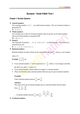
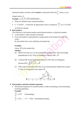
This document provides a summary of key concepts from Grade 9 Math Term I, including: - Different types of numbers (natural, whole, integers, rational, irrational, real) and their properties - Polynomials, including definitions of terms, degrees, zeros, and factoring polynomials - The Cartesian coordinate system for identifying points on a plane using perpendicular x and y axes, with the origin at their intersection

1. Synopsis – Grade 9 Math Term I
Chapter 1: Number Systems
 Natural numbers
The counting numbers 1, 2, 3 … are called natural numbers. The set of natural numbers is
denoted by N.
N = {1, 2, 3…}
 Whole numbers
If we include zero to the set of natural numbers, then we get the set of whole numbers.
The set of whole numbers is denoted by W.
W = {0, 1, 2…}
 Integers
The collection of numbers … –3, –2, –1, 0, 1, 2, 3 … is called integers. This collection is
denoted by Z, or I.
Z = {…, –3, –2, –1, 0, 1, 2, 3…}
 Rational numbers
p
Rational numbers are those which can be expressed in the form , where p, q are integers
q
and q  0.
1 3 6
Example: , , , etc.
2 4 9
a
, where a, b are integers such that
b

Every rational number „x ‟can be expressed as x 


the HCF of a and b = 1 and b  0.
Every natural number, whole number or integer is a rational number.
There are infinitely many rational numbers between any two given rational numbers.
Example:
Find a rational number between
3
5
and
.
8
12
Solution:
The mean of two given rational numbers gives a rational number between them.
3 5 19
Now,  
8 12 24
3 5 
   19
3
5
8 12 

 A rational number between and
= 
2
48
8
12
 Irrational numbers

2. Irrational numbers are those which cannot be expressed in the form
p
, where p, q are
q
integers and q  0.
Example: π, 2, 7, 14,0.0202202220.......

There are infinitely many irrational numbers.

π = 3.141592… is irrational. Its approximate value is assumed as
22
or as 3.14, both
7
of which are rational.
 Real numbers
The collection of all rational numbers and irrational numbers is called real numbers.
 A real number is either rational or irrational.
 Every real number is represented by a unique point on the number line (and vice
versa).
So, the number line is also called the real number line.
Example:
Locate 6 on the number line.
Solution:
(a) Mark O at 0 and A at 2 on the number line, and then draw AB of unit length
perpendicular to OA. Then, by Pythagoras Theorem, OB  5
(b)
Construct BD of unit length perpendicular to OB. Thus, by Pythagoras
theorem, OD 
(c)
 5  12 
2
6
With centre O and radius OD, draw an arc intersecting the number line at point
P. Thus, P corresponds to the number 6 .
 Real numbers and their decimal expansions
 The decimal expansion of a rational number is either terminating or non-terminating
recurring (repeating).
Example:
15
 1.875
 Terminating 
8
4
 1.333.......  1.3  Non – terminating recurring 
3

3. 
A number whose decimal expansion is terminating or non-terminating repeating is
rational.
 The decimal expansion of an irrational number is non-terminating non-recurring.
Moreover, a number whose decimal expansion is non-terminating non- recurring is
irrational.
Example:
2.645751311064……. is an irrational number
 Representation of real numbers on the number line
Example: 3.32 can be visualize by the method of successive magnification on the number
line as follows:
 Operation on real numbers
 The sum or difference of a rational number and an irrational number is always
irrational.
 The product or quotient of a non-zero rational number with an irrational number is
always irrational.
 If we add, subtract, multiply or divide two irrational numbers, then the result may be
rational or irrational.
 Identities
If a and b are positive real numbers, then

ab  a b

a
a

b
b

4. 


 a  b  a  b   a


a b



a b

a b


a  b  a  b2
2
2
b

c  d  ac  ad  bc  bd
 a  2 ab  b
 Rationalisation of denominator
The denominator of
a b
can be rationalised by multiplying both the numerator and
x y
the denominator by x  y , where a, b, x, y are integers.
 Laws of exponents
Let a > 0 is a real number and p, q are rational numbers.

a p .a q  a p q

a 

ap
 a pq
aq

 ab 

x
p
q
p
 a pq
 a pb p
1
x
a  a , where n is a positive integer.
Chapter 2: Polynomials
 Polynomial in one variable
A polynomial p(x) in one variable i.e., x is an algebraic expression in x of the form
p  x   an xn  an1 xn1  .....  a1 x  a0 , where a0 , a1 ... an are constants and an  0 .
a0 , a1 ... an are the respective coefficients of x0 , x1 , x 2 ... x n and n is called the degree of
the polynomial. an x n , an1 x n1 ... a0 and a0  0 are called the terms of p(x).

5.  Constant polynomial: A constant polynomial is of the form p  x   k , where k is a real
number. For example, –9, 10, 0 are constant polynomials.
 The degree of a non-zero constant polynomial is zero.
 Zero polynomial: A constant polynomial „0‟ is called zero polynomial.
 The degree of a zero polynomial is not defined.
 Classification of polynomials according to terms
 A polynomial comprising one term is called a monomial, e.g., 3x, 5, 25t3.
 A polynomial comprising two terms is called a binomial, e.g., 2t – 6, 3x4 + 2x etc.
 A polynomial comprising three terms is called a trinomial, e.g.,
 x3  5x  2, y 6  y  9.
 Classification of polynomial according to their degrees
 A polynomial of degree one is called a linear polynomial, e.g., 3x+ 2, 4x, x + 9.
 A polynomial of degree two is called a quadratic polynomial, e.g., x 2  9 ,

3x 2  4 x  6 .
A polynomial of degree three is called a cubic polynomial, e.g., 10 x3  3, 9 x3 .
 Zeroes of a polynomial: A real number  is said to be the zero of polynomial p  x  if
p    0 . In this case,  is also called the root of the equation p  x   0




A non-zero constant polynomial has no zeroes
Every real number is a zero of the zero polynomial
The maximum number of zeroes of a polynomial is equal to the degree of the
polynomial
A polynomial can have more than one zeroes
Example: Find the value of polynomial p  x   3x3  2 x  9 at x  2 .
Solution:
p  x   3x3  2 x  9
 p  2   3  2   2  2   9
3
 24  4  9  19
Thus, x = –2 is not the zero of the polynomial.
 Division of a polynomial by another polynomial
If p(x) and g(x) are two polynomials such that degree of p(x)  degree of g  x  and
g  x   0 , then we can find polynomials q  x  and r  x  such that
p  x   g  x  q  x   r  x  , where r  x   0 or degree of r  x  < degree of g(x)
Here, p(x) is the dividend, g  x  is the divisor, q  x  is the quotient, and r  x  is the
remainder.
Example: Divide x4  2 x3  2 x2  7 x  15 by x – 2.
Solution:

6. x3  2 x  3
x2
x 4  2 x 3  2 x 2  7 x  15
x 4  2 x3
 
 2 x 2  7 x  15
 2x2  4x


3 x  15
3x  6
 
9




It can be easily verified that x4  2 x3  2 x 2  7 x  15   x  2  x3  2 x  3   9  .
 Remainder theorem
If p(x) is a polynomial of degree greater than or equal to one and a is a real number, then,
when p(x) is divided by linear polynomial x – a, the remainder is p(a).
 Factor theorem: If p(x) is a polynomial of degree x  1and a is any real number, then
 x – a is a factor of p(x), if p(a) = 0
 p  a   0 , if  x  a  is a factor of p(x)
 Factorisation of polynomials: Polynomials can be factorised by using the algebraic
identities given below.

 x  y


 x  y   x2  2xy  y 2
 x  y  x  y   x2  y 2
 x  a  x  b   x2   a  b  x  ab

 x  y  z

 x  y
3
 x3  y 3  3xy  x  y   x3  y 3  3x 2 y  3xy 2

 x  y
3
 x3  y 3  3xy  x  y   x3  y3  3x2 y  3xy 2

x3  y3  z 3  3xyz   x  y  z  x 2  y 2  z 2  xy  yz  zx

2
 x 2  2 xy  y 2
2
2
 x 2  y 2  z 2  2 xy  2 yz  2 zx


For example: Factorise 4 x 2  20 xy  25 y 2
4 x 2  20 xy  25 y 2   2 x   2  2 x  5 y   5 y 
2
  2x  5 y 
2
  2 x  5 y  2 x  5 y 
2
 a 2  2ab  b 2   a  b 2 



7. Chapter 3: Coordinate Geometry
 To identify the position of an object or a point in a plane, we require two perpendicular
lines: one of them is horizontal and the other is vertical.
 Cartesian system
 A Cartesian system consists of two perpendicular lines: one of them is horizontal and
the other is vertical.
 The horizontal line is called the x- axis and the vertical line is called the y -axis.
XOX is called the x-axis; YOY is called the y-axis
 The point of intersection of the two lines is called origin, and is denoted by O.

OX and OY are respectively called positive x-axis and positive y-axis.
Positive numbers lie on the directions of OX and OY.
 OX and OY are respectively called negative x-axis and negative y-axis.
 The axes divide the plane into four equal parts.
The four parts are called quadrants, numbered I, II, III and IV, in anticlockwise from
positive x-axis, OX.
 The plane is also called co-ordinate plane or Cartesian plane or xy -plane.
 The coordinates of a point on the coordinate plane can be determined by the
following conventions.
 The x-coordinate of a point is its perpendicular distance from the y-axis, measured
along the x-axis (positive along the positive x-axis and negative along the negative xaxis).
The x-coordinate is also called the abscissa.

8. 



The y-coordinate of a point is its perpendicular distance from the x-axis, measured
along the y-axis ( positive along the positive y-axis and negative along the negative y axis)
The y-coordinate is also called the ordinate.
In stating the coordinates of a point in the coordinate plane, the x-coordinate comes
first and then the y-coordinate. The coordinates are placed in brackets.
If x = y, then (x, y) = ( y, x); and (x, y)  (y, x) if x  y.
The coordinates of the origin are (0, 0). Since the origin has zero distance from both
the axes, its abscissa and ordinate are both zero.
The coordinates of the point on the x-axis are of the form (a, 0) and the coordinates of
the point on the y-axis are of the form (0, b), where a, b are real numbers.
Example: What are the coordinates of points A and C in the given figure?
Solution:
It is observed that
x-coordinate of point A is 5
y-coordinate of point A is 2
Coordinates of point A are (5, 2)
x-coordinate of point C is –5
y-coordinate of point C is 2
Coordinates of point C are (–5, 2)
 Relationship between the signs of the coordinates of a point and the quadrant of the
point in which it lies:
 The 1st quadrant is enclosed by the positive x-axis and positive y-axis. So, a point in
the 1st quadrant is in the form (+, +).

9. 
The 2nd quadrant is enclosed by the negative x-axis and positive y-axis. So, a point in
the 2nd quadrant is in the form (–, +).
 The 3rd quadrant is enclosed by the negative x-axis and the negative y-axis. So, the
point in the 3rd quadrant is in the form (–, –).
 The 4th quadrant is enclosed by the positive x-axis and the negative y-axis. So, the
point in the 4th quadrant is in the form (+, –).
 Location of a point in the plane when its coordinates are given
Example: Plot the following ordered pairs of numbers (x, y) as points in the coordinate
plane.
x
y
–3
4
4
–3
–3
–3
0
2
Solution:
These points can be located in the coordinate plane as:
Chapter 5: Introduction to Euclid’s Geometry
 Introduction to Euclid’s geometry
During Euclid‟s period, the notions of points, line, plane (or surface), and so on were
derived from what was seen around them.
 Euclid’s definitions
Some definitions given in his book I of the „Elements‟ are as follows.
 A point is that which has no part.

10.  A line is breadth-less length.
 A straight line is a line which lies evenly with the points on itself.
 A surface is that which has length and breadth only.
 The edges of a surface are lines.
 A plane surface is a surface which lies evenly with the straight lines on itself.
In the above definitions, we can observe that some of the terms such as part, breadth,
length, etc. require better explanations.
Therefore, to define one thing, we require defining many other things and we may obtain
a long chain of definitions without an end. For such reasons, mathematicians agreed to
leave some geometric terms such as point, line, and plane undefined.
 Euclid’s axioms and postulates
Axioms and postulates are the assumptions that are obvious universal truths, but are not
proved. Euclid used the term “postulate” for the assumptions that were specific to
geometry whereas axioms are used throughout mathematics and are not specifically
linked to geometry.
 Some of Euclid’s axioms
 Things that are equal to the same things are equal to one another.
 If equals are added to equals, then the wholes are also equal.
 If equals are subtracted from equals, then the remainders are equal.
 Things that coincide with one another are equal to one another.
 The whole is greater than the part.
 Things that are double of the same things are equal to one another.
 Things that are halves of the same things are equal to one another.
 Euclid’s five postulates
Postulate 1: A straight line may be drawn from any one point to any other point.
Euclid has frequently assumed this postulate, without mentioning that there is a unique
line joining two distinct points. The above result can be stated in the form of an axiom as
follows.
Axiom: Given two distinct points, there is a unique line that passes through them.
Postulate 2: A terminated line can be produced indefinitely.
The second postulate states that a line segment can be extended on either side to form a
line.
Postulate 3: A circle can be drawn with any centre and any radius.
Postulate 4: All right angles are equal to one another.
Postulate 5: If a straight line falling on two straight lines makes the interior angles on the
same side of it taken together less than two right angles, then the two straight lines, if
produced indefinitely, meet on that side on which the sum of angles is less than two right
angles.
 A system of axioms is called consistent, if it is impossible to deduce a statement from
these axioms that contradicts any axiom or previously proved statement.
Therefore, when a system of axioms is given, it has to be ensured that the system is
consistent.

11.  Propositions or theorems
Propositions or theorems are statements that are proved, using definitions, axioms,
previously proved statements, and deductive reasoning.
Theorem: Two distinct lines cannot have more than one point in common.
This theorem can be proved by using the axiom, “There is a unique line passing through
two distinct points”.
 Equivalent versions of Euclid’s fifth postulate
Two equivalent versions of Euclid‟s fifth postulate are as follows.
 For every line l and for every point p not lying on l, there exists a unique line „m‟
passing through p and parallel to l.
 Two distinct intersecting lines cannot be parallel to the same line.
The attempts to prove Euclid‟s fifth postulate as a theorem have failed. However, their
efforts have led to the discovery of several other geometries called non-Euclidean
geometries.
 Non-Euclidean geometry is also called spherical geometry. In spherical geometry, lines
are not straight. They are part of great circles (that is, circles obtained by the intersection
of a sphere and planes passing through the centre of the sphere).
Chapter 6: Lines and Angles
 A pair of angles whose sum is 90 is called complementary angles.
Example: 40 and 50 are complementary angles.
 A pair of angles whose sum is 180 is known as supplementary angles.
Example: 60 and 120 are supplementary angles.
 If two lines intersect each other
 The pairs of opposite angles so formed are called pairs of vertically opposite angles.
 Vertically opposite angles are equal in measure
Example: In the following figure, AOD and BOC, AOC and BOD are the pairs of
vertically opposite angles.
 AOD = BOC and AOC = BOD
 Two angles are said to be adjacent angles, if they have a common arm.
In the given figure, AOB and BOC are adjacent angles.

12.  A pair of angles is called a linear pair, if they are adjacent and supplementary.
In the given figure, ABD and CBD are linear pair of angles.
It can be said that if a ray stands on a line, then the two angles so formed are a linear pair
of angles.
 Transversal is a line which intersects two or more lines at distinct points.
 When a transversal intersects two lines l and m, the angles so formed at the intersection
points are named as follows.

Corresponding angles
1 and 5, 2 and 6, 3 and 7, 4 and 8
 Alternate interior angles
3 and 5, 4 and 6
 Alternate exterior angles
1 and 7, 2 and 8
 Corresponding angle axiom and its converse
If a transversal intersects two parallel lines, then each pair of corresponding angles is
equal.
Its converse is also true.
If a transversal intersects two lines such that a pair of corresponding angles is equal, then
the two lines are parallel to each other.

13. In the following figure, the corresponding angles are equal. Therefore, the lines l and m
are parallel to each other.
 Alternate angle axiom and its converse
If a transversal intersects two parallel lines, then each pair of alternate angles is equal.
Its converse is also true.
If a transversal intersects two lines such that a pair of alternate angles is equal, then the
two lines are parallel to each other.
In the following figure, a pair of alternate angles is equal. Therefore, l and m are parallel
lines.
 Angles on the same side of transversal
If a transversal intersects two parallel lines, then each pair of angles on the same side of
the transversal are supplementary.
Its converse states that if a transversal intersects two lines such that each pair of interior
angles on the same side of the transversal are supplementary, then the two lines are
parallel to each other.
In the following figure, if 1 + 4 = 180 or 2 + 3 = 180, then it can be said that
lines l and m are parallel to each other.

14.  Lines that are parallel to the same line are parallel to each other.
In the following figure, if AB||CD and CD||EF, then AB||EF.
 Lines that are perpendicular to the same line are parallel to each other.
In the following figure, CEAB and DFAB. Hence, CE||DF.
 Angle sum property
The sum of all the three interior angles of a triangle is 180.

15.  A + B + C = 180
 Exterior angle property
If a side of a triangle is produced, then the exterior angle so formed is equal to the sum of
the two interior opposite angles.
ACX = BAC + ABC.
Chapter 7: Triangles
 Two figures are said to be congruent if they are of the same shape and size.
 Similar figures are of the same shape but not necessarily of the same size.
 If ABC  XYZ, then
 AB = XY, BC = YZ, AC = XZ
 A = X, B = Y, and C = Z.
Corresponding parts of congruent triangles are equal.
 SAS congruence rule
If two sides and the included angle of one triangle are equal to the two sides and the
included angle of the other triangle, then the two triangles are congruent to each other.
 ASA congruence rule
If two angles and the included side of a triangle are equal to the two angles and the
included side of the other triangle, then the two triangles are congruent to each other.
 AAS congruence rule
If two angles and one side of a triangle are equal to two angles and the corresponding side
of the other triangle, then the two triangles are congruent to each other.
 SSS congruence rule
If three sides of a triangle are equal to the three sides of the other triangle, then the two
triangles are congruent.
 RHS congruence rule
If the hypotenuse and one side of a right triangle are equal to the hypotenuse and one side
of the other right triangle, then the two triangles are congruent to each other.
 Properties of isosceles triangles
 Angles opposite to equal sides of a triangle are equal.
 Sides opposite to equal angles of a triangle are equal in length.

16.  Inequalities in a triangle
 Angle opposite to the longer side of a triangle is greater.
 Side opposite to the greater angle of a triangle is longer.
 The sum of any two sides of a triangle is greater than the third side.
 The difference of any two sides of a triangle is smaller than the third side.
Chapter 12: Heron’s Formula
 Heron’s formula
When all the three sides of a triangle are given, its area can be calculated by Heron‟s
formula.
Let a, b, and c be the sides of a triangle.
abc
 Semi-perimeter of the triangle and is given by, s 
2

Area of triangle = s  s  a  s  b  s  c 
Example: What is the area of a triangle whose sides are 9 cm, 28 cm, and 35 cm?
Solution: Let a = 9 cm, b = 28 cm, and c = 35 cm
a  b  c  9  28  35 
Semi-perimeter, s 

 cm  36 cm
2
2


Area of triangle  36  36  9  36  28 6  35 cm2
 36  27  8 1 cm 2
 36 6 cm 2
 Area of a quadrilateral can also be calculated using Heron‟s formula. Firstly, the
quadrilateral is divided into two triangles. Then, the area of each triangle is calculated
using Heron‟s formula.