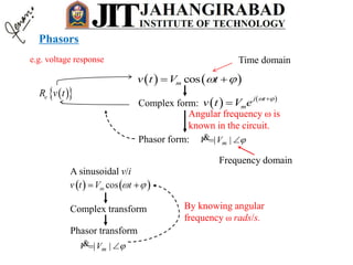
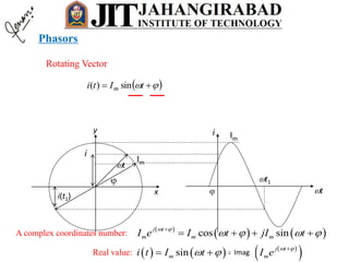
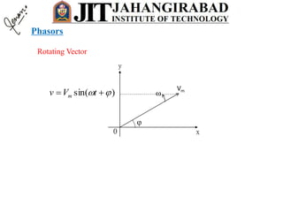
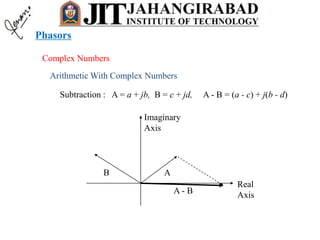
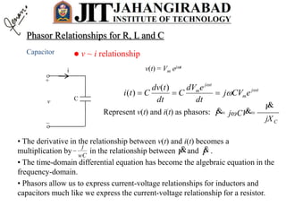
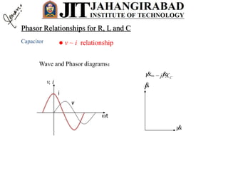
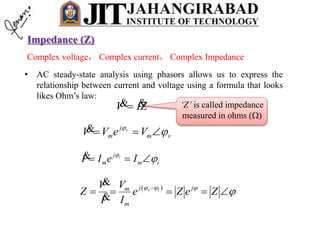
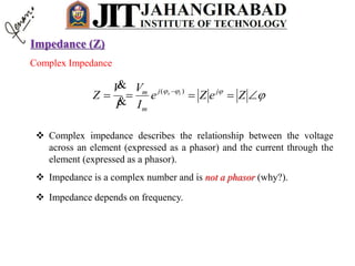
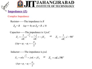
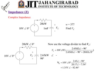
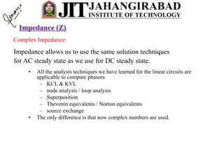
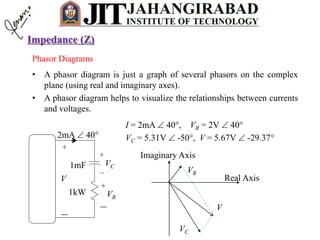
- Any steady state voltage or current in a linear circuit with a sinusoidal source is a sinusoid with the same frequency as the source. Phasors and complex impedances allow conversion of differential equations to circuit analysis by representing magnitude and phase of sinusoids.
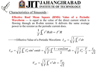
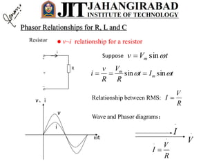
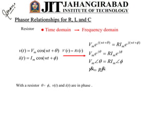
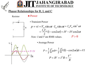
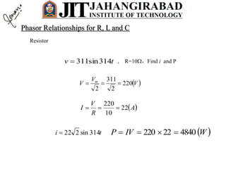
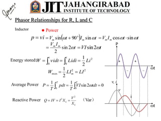
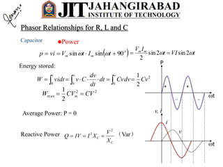
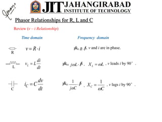
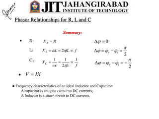
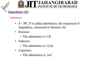
- For a resistor, the voltage and current are in phase. In the phasor domain, the resistor phasor relationship is V=IR. In the time domain, the average power dissipated is proportional to the product of RMS current and voltage.
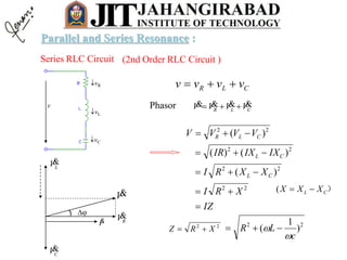
( CL XXjR
I
V
Z
ZjXRZ
22
)( CL XXRZ
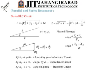
R
XX CL
1
tan
iv
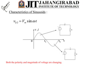
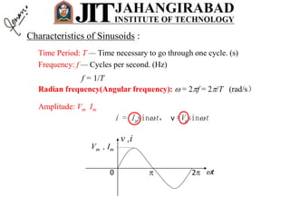
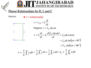
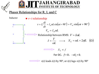
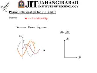
v
vR
vL
vC
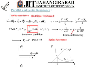
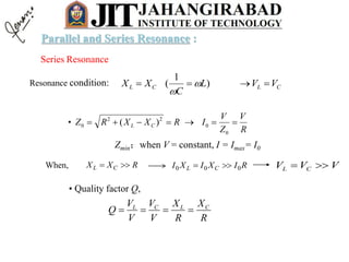
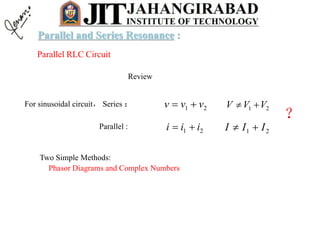
Series RLC Circuit
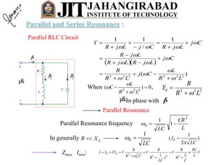
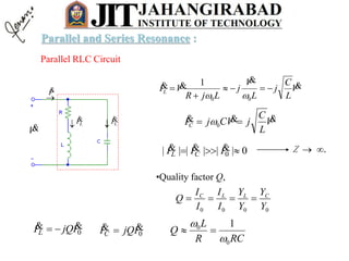
Parallel and Series Resonance :](https://image.slidesharecdn.com/acsinglephase-161231060524/85/Ac-single-phase-54-320.jpg)