This document provides an overview of a book on maintenance theory of reliability by Toshio Nakagawa. The book discusses maintenance policies for system reliability models, focusing on repair, preventive maintenance, replacement, and inspection policies. It aims to summarize research results on standard and advanced problems in maintenance policies. The book is composed of nine chapters covering topics like repair maintenance, age replacement, periodic replacement, block replacement, preventive maintenance policies, imperfect maintenance models, and inspection policies. It provides mathematical formulations and optimization techniques for maintenance problems.


![1
Introduction
Reliability theory has grown out of the valuable experiences from many de-
fects of military systems in World War II and with the development of modern
technology. For the purpose of making good products with high quality and
designing highly reliable systems, the importance of reliability has been in-
creasing greatly with the innovation of recent technology. The theory has
been actually applied to not only industrial, mechanical, and electronic engi-
neering but also to computer, information, and communication engineering.
Many researchers have investigated statistically and stochastically complex
phenomena of real systems to improve their reliability.
Recently, many serious accidents have happened in the world where sys-
tems have been large-scale and complex, and they not only caused heavy
damage and a social sense of instability, but also brought an unrecoverable
bad influence on the living environment. These are said to have occurred from
various sources of equipment deterioration and maintenance reduction due to
a policy of industrial rationalization and personnel cuts.
Anyone may worry that big earthquakes in the near future might happen
in Japan and might destroy large old plants such as chemical and power plants,
and as a result, inflict serious damage to large areas.
Most industries at present restrain themselves from making investments in
new plants and try to run current plants safely and efficiently as long as possi-
ble. Furthermore, advanced nations have almost finished public infrastructure
and will now rush into a maintenance period [1]. From now on, maintenance
will be more important than redundancy, production, and construction in
reliability theory, i.e., more maintenance than redundancy and more mainte-
nance than production. Maintenance policies for industrial systems and public
infrastructure should be properly and quickly established according to their
occasions. From these viewpoints, reliability researchers, engineers, and man-
agers have to learn maintenance theory simply and throughly, and apply them
to real systems to carry out more timely maintenance.
The book considers systems that perform some mission and consist of
several units, where unit means item, component, part, device, subsystem,
1](https://image.slidesharecdn.com/maintenancetheoryofreliabilityspringerseriesinreliability-240303085250-86c4adaf/85/Maintenance_Theory_of_Reliability_Springer_Series_in_Reliability-pdf-10-320.jpg)

![1 Introduction 3
We need to check units such as standby and storage units whose failures
can be detected only through inspection, which is called inspection policy.
For example, consider the case where a standby unit may fail. It may be
catastrophic and dangerous that a standby unit has failed when an original
unit fails. To avoid such a situation, we should check a standby unit to see
whether it is good. If the failure is detected then the maintenance suitable for
the unit should be done immediately.
Most systems in offices and industry are successively executing jobs and
computer processes. For such systems, it would be impractical to do mainte-
nance on them at planned times. Random replacement and inspection policies,
in which units are replaced and checked, respectively, at random times, are
proposed in Chapter 9.
For systems with redundant or spare units, we have to determine how
many units should be provided initially. It would not be advantageous to hold
too many units in order to improve reliability, or to hold too few units in order
to reduce costs. As one technique of determining the number of units, we may
compute an optimum number of units that minimize the expected cost, or the
minimum number such that the probability of failure is less than a specified
value. If the total cost is given, we may compute the maximum number of
units within a limited cost. Furthermore, we are interested in an optimization
problem: when to replace units with spare ones in order to lengthen the time
to failure.
Failures occur in several different types of failure modes such as wear,
fatigue, fracture, crack, breaking, corrosion, erosion, instability, and so on.
Failure is classified into intermittent failure and extended failure [2, 3]. Fur-
thermore, extended failure is divided into complete failure and partial failure,
both of which are classified into sudden failure and gradual failure. Extended
failure is also divided into catastrophic failure which is both sudden and com-
plete, and degraded failure which is both partial and gradual.
In such failure studies, the time to failure is mostly observed on operating
time or calendar time, however, it is often measured by the number of cycles
to failure and combined scales. A good time scale of failure maintenance mod-
els was discussed in [4, 5]. Furthermore, alternative time scales for cars with
random usage were defined and investigated in [6]. In other cases, the lifetimes
are sometimes not recorded at the exact instant of failure and are collected
statistically at discrete times. Rather some units may be maintained preven-
tively in their idle times, and intermittently used systems maintained after
a certain number of uses. In any case, it would be interesting and possibly
useful to solve optimization problems with discrete times.
It is supposed that the planning time horizon for most units is infinite. In
this case, as the measures of reliability, we adopt the mean time to failure, the
availability, and the expected cost per unit of time. It is appropriate to adopt
as objective functions the expected cost from the viewpoint of economics, the
availability from overall efficiency, and the mean time to failure from reliability.
Practically, the working time of units may be finite. The total expected cost](https://image.slidesharecdn.com/maintenancetheoryofreliabilityspringerseriesinreliability-240303085250-86c4adaf/85/Maintenance_Theory_of_Reliability_Springer_Series_in_Reliability-pdf-12-320.jpg)
![4 1 Introduction
until maintenance is adopted for a finite time interval as an objective function,
and optimum policy that minimizes it is discussed by using the partition
method derived in Chapter 8.
The known results of maintenance and associated optimization problems
were summarized in [7–11]. Since then, many papers have been published
and reviewed in [12–19]. The recently published books [20–25] collected many
reliability and maintenance models, discussed their optimum policies, and
applied them to actual systems.
Most of the contents of this book are our original work based on the book of
Barlow and Proschan: reliability measures, failure distributions, and stochas-
tic processes needed for learning reliability theory are summarized briefly in
Chapter 1. These results are introduced without detailed explanations and
proofs. However, several examples are given to help us to understand them
easily.
Some fundamental repair models in reliability theory are analyzed in Chap-
ter 2, and useful reliability quantities of such repairable systems are analyti-
cally obtained, using the techniques in Chapter 1. Several replacement policies
are contained systematically from elementary knowledge to advanced studies
in Chapters 3 through 5. Several preventive maintenance and imperfect poli-
cies are introduced and analyzed in Chapters 6 and 7. The results and methods
presented in Chapters 3 through 7 can be applied practically to real systems
by modifying and extending them according to circumstances. Moreover, they
might include scholarly research materials for further studies. The most im-
portant thing in reliability engineering is when to check units suitably and
how to seek fitting maintenance for them. Many inspection models based on
the results of Barlow and Proschan are summarized in Chapter 8, and would
be useful for us to plan maintenance schemes and to carry them into execu-
tion. Finally, several modified maintenance models are surveyed in Chapter 9,
and give further topics of research.
1.1 Reliability Measures
We are interested in certain quantities for analyzing reliability and mainte-
nance models. The first problem is that of how long a unit can operate without
failure, i.e., reliability, which is defined as the probability that it will perform
a required function under stated conditions for a stated period of time [26].
Failure might be defined in many ways, and usually means mechanical break-
down, deterioration beyond a threshold level, appearance of certain defects
in system performance, or decrease in system performance below a critical
level [4]. Failure rate is a good measure for representing the operating charac-
teristics of a unit that tends to frequency as it ages. When units are replaced
upon failure or are preventively maintained, we are greatly concerned with
the ratio at which units can operate, i.e., availability, which is defined as the](https://image.slidesharecdn.com/maintenancetheoryofreliabilityspringerseriesinreliability-240303085250-86c4adaf/85/Maintenance_Theory_of_Reliability_Springer_Series_in_Reliability-pdf-13-320.jpg)
![1.1 Reliability Measures 5
probability that it will be able to operate within the tolerances at a given
instant of time [27].
This section defines reliability function, failure rate, and availability, and
obtains their properties needed for solving future optimization problems of
maintenance policies, which are treated in the sequel chapters.
(1) Reliability
Suppose that a nonnegative random variable X (X ≥ 0) which denotes
the failure time of a unit, has a cumulative probability distribution F(t) ≡
Pr{X ≤ t} with right continuous, and a probability density function f(t)
(0 ≤ t < ∞); i.e., f(t) = dF(t)/dt and F(t) =
t
0
f(u)du. They are called
failure time distribution and failure density function in reliability theory, and
are sometimes called simply a failure distribution F(t) and a density function
f(t).
The survival distribution of X is
R(t) ≡ Pr{X t} = 1 − F(t) =
∞
t
f(u) du ≡ F(t) (1.1)
which is called the reliability function, and its mean is
µ ≡ E{X} =
∞
0
tf(t) dt =
∞
0
R(t) dt (1.2)
if it exists, which is called MTTF (mean time to failure) or mean lifetime. It is
usually assumed throughout this book that 0 µ ∞, F(0−) = F(0+) = 0,
and F(∞) = limt→∞ F(t) = 1; i.e., R(0) = 1 and R(∞) = 0, unless otherwise
stated. Note that F(t) is nondecreasing from 0 to 1 and R(t) is nonincreasing
from 1 to 0.
(2) Failure Rate
The notion of aging, which describes how a unit improves or deteriorates
with its age, plays a role in reliability theory [28]. Aging is usually measured
based on the term of a failure rate function. That is, failure rate is the most
important quantity in maintenance theory, and important in many different
fields, e.g., statistics, social sciences, biomedical sciences, and finance [29–31].
It is known by different names such as hazard rate, risk rate, force of mortality,
and so on [32]. In particular, Cox’s proportional hazard model is well known
in the fields of biomedical statistics and default risk [33, 34]. The existing
literature on this model was reviewed in [35].
We define instant failure rate function h(t) as
h(t) ≡
f(t)
F(t)
= −
1
F(t)
dF(t)
dt
for F(t) 1 (1.3)](https://image.slidesharecdn.com/maintenancetheoryofreliabilityspringerseriesinreliability-240303085250-86c4adaf/85/Maintenance_Theory_of_Reliability_Springer_Series_in_Reliability-pdf-14-320.jpg)
![6 1 Introduction
which is called simply the failure rate or hazard rate. This means physically
that h(t)∆t ≈ Pr{t X ≤ t+∆t|X t} represents the probability that a unit
with age t will fail in an interval (t, t + ∆t] for small ∆t 0. This is generally
drawn as a bathtub curve. Recently, the reversed failure rate is defined by
f(t)/F(t) for F(t) 0, where f(t)∆t/F(t) represents the probability of a
failure in an interval (t − ∆t, t] given that it has occurred in (0, t] [36,37].
Furthermore, H(t) ≡
t
0
h(u)du is a cumulative hazard function, and has
the relation
R(t) = exp
−
t
0
h(u) du
= e−H(t)
; i.e., H(t) = − log R(t). (1.4)
Thus, F(t), R(t), f(t), h(t), and H(t) determine one another. In addition,
because ea
≥ 1 + a, we have the inequalities
H(t)
1 + H(t)
≤ F(t) ≤ H(t) ≤
F(t)
1 − F(t)
which would give good inequalities for small t 0.
In particular, a random variable Y ≡ H(X) has the following distribution
Pr{Y ≤ t} = Pr{H(X) ≤ t} = Pr{X ≤ H−1
(t)} = 1 − e−t
,
where H−1
is the inverse function of H. Thus, Y has an exponential distribu-
tion with mean 1, and E{H(X)} = 1. Moreover, x1 which satisfies H(x1) = 1
is called characteristic life in the probability paper of a Weibull distribution.
This represents the mean lifetime that about 63.2% of units have failed until
time x1. Moreover, H(t) is called the mean value function and has a close re-
lation to nonhomogeneous Poisson processes in Section 1.3. In this process, xk
which satisfies H(xk) = k (k = 1, 2, . . . ) represents the time that the expected
number of failures is k when failures occur at a nonhomogeneous Poisson pro-
cess. The property of H(t)/t, which represents the expected number of failures
per unit of time, was investigated in [38].
We denote the following failure rates of a continuous failure distribution
F(t) and compare them [39,40].
(1) Instant failure rate h(t) ≡ f(t)/F(t).
(2) Interval failure rate h(t; x) ≡
t+x
t
h(u) du/x = log[F(t)/F(t + x)]/x for
x 0.
(3) Failure rate λ(t; x) ≡ [F(t + x) − F(t)]/F(t) for x 0.
(4) Average failure rate Λ(t; x) ≡ [F(t + x) − F(t)]/
t+x
t
F(u)du for x 0.
Definition 1.1. A distribution F is IFR (DFR) if and only if λ(t; x) is
increasing (decreasing) in t for any given x 0 [7], where IFR (DFR) means
Increasing Failure Rate (Decreasing Failure Rate).
By this definition, we investigate the properties of failure rates.](https://image.slidesharecdn.com/maintenancetheoryofreliabilityspringerseriesinreliability-240303085250-86c4adaf/85/Maintenance_Theory_of_Reliability_Springer_Series_in_Reliability-pdf-15-320.jpg)
![1.1 Reliability Measures 7
Theorem 1.1.
(i) If one of the failure rates is increasing (decreasing) in t then the others
are increasing (decreasing), and if F is exponential, i.e., F(t) = 1 − e−λt
,
then all failure rates are constant in t, and h(t) = h(t; x) = Λ(t; x) = λ.
(ii) If F is IFR then Λ(t−x; x) ≤ h(t) ≤ Λ(t; x) ≤ h(t+x), where Λ(t−x; x) =
Λ(0; t) for x t.
(iii) If F is IFR then Λ(t; x) ≤ h(t; x).
(iv) h(t; x) ≥ λ(t; x)/x and Λ(t; x) ≥ λ(t; x)/x.
(v) h(t) = limx→0 h(t; x) = limx→0 λ(t; x)/x = limx→0 Λ(t; x).
Proof. The property (v) easily follows from the definition of h(t). Hence,
we can prove property (i) if we show that h(t) is increasing (decreasing) in
t implies h(t; x), λ(t; x), and Λ(t; x) all are increasing (decreasing) in t. For
example, for t1 ≤ t2,
F(t1 + x)
F(t1)
= exp
−
t1+x
t1
h(u) du
≥ (≤) exp
−
t2+x
t2
h(u) du
=
F(t2 + x)
F(t2)
implies that λ(t; x) is increasing (decreasing) if h(t) is increasing (decreasing).
Similarly, we can prove the other properties.
Suppose that F is IFR. Because
f(v)
F(v)
≤ h(t) ≤
f(u)
F(u)
≤ h(t + x) for v ≤ t ≤ u ≤ t + x
we easily have property (ii).
Furthermore, letting
Q(x) ≡
t+x
t
h(u) du
t+x
t
F(u) du − x[F(t + x) − F(t)]
we have Q(0) = 0, and
dQ(x)
dx
=
t+x
t
[h(t + x) − h(u)][F(t + x) − F(u)] du ≥ 0
because both h(t) and F(t) are increasing in t. This proves property (iii).
Finally, from the property that F(t) is decreasing in t, we have
t+x
t
F(u) du ≤ xF(t),
t+x
t
f(u)
F(u)
du ≥
1
F(t)
t+x
t
f(u) du
which imply property (iv). All inequalities in results (ii) and (iii) are reversed
when F is DFR.
Hereafter, we may call the four failure rates simply the failure rate or
hazard rate. Furthermore, properties of failure rates have been investigated
in [8,28,41].](https://image.slidesharecdn.com/maintenancetheoryofreliabilityspringerseriesinreliability-240303085250-86c4adaf/85/Maintenance_Theory_of_Reliability_Springer_Series_in_Reliability-pdf-16-320.jpg)
![8 1 Introduction
Example 1.1. Consider a unit such as a scale and production system that
is maintained preventively only at time T (0 ≤ T ≤ ∞). It is supposed that
an operating unit has some earnings per unit of time and does not have any
earnings during the time interval if it fails before time T. The average time
during (0, T] in which we have some earnings is
l0(T) = 0 × F(T) + TF(T) = TF(T)
and l0(0) = l0(∞) = 0. Differentiating l0(T) with respect to T and setting it
equal to zero, we have
F(T) − Tf(T) = 0; i.e., h(T) =
1
T
.
Thus, an optimum time T0 that maximizes l0(T) is given by a unique solution
of equation h(T) = 1/T when F is IFR. For example, when F(t) = 1 − e−λt
,
T0 = 1/λ; i.e., we should do the preventive maintenance at the interval of
mean failure time.
Next, consider a unit with one spare where the first operating unit is
replaced before failure at time T (0 ≤ T ≤ ∞) with the spare one which
will be operating to failure. Suppose that both units have the identical failure
distribution F(t) with finite mean µ. Then, the mean time to either failure of
the first or spare unit is
l1(T) =
T
0
t dF(t) + F(T)(T + µ) =
T
0
F(t) dt + F(T)µ
and l1(0) = l1(∞) = µ, and
dl1(T)
dT
= F(T)[1 − µh(T)].
Thus, an optimum time T1 that maximizes l1(T) when h(t) is strictly increas-
ing is given uniquely by a solution of equation h(T) = 1/µ. When the failure
rate of parts and machines is statistically estimated, T0 and T1 would be a
simple barometer for doing their maintenance.
A generalized model with n spare units is discussed in Section 9.4. A prob-
ability method of provisioning spare parts and several models for forecasting
spare requirements and integrating logistics support were provided and dis-
cussed in [42,43].
Example 1.2. Suppose that X denotes the failure time of a unit. Then, the
failure distribution of a unit with age T (0 ≤ T ∞) is F(t; T) ≡ Pr{T
X ≤ t + T|X T} = λ(T; t) = [F(t + T) − F(T)]/F(T), and its MTTF is
∞
0
F(t; T) dt =
1
F(T)
∞
T
F(t) dt (1.5)](https://image.slidesharecdn.com/maintenancetheoryofreliabilityspringerseriesinreliability-240303085250-86c4adaf/85/Maintenance_Theory_of_Reliability_Springer_Series_in_Reliability-pdf-17-320.jpg)
![1.1 Reliability Measures 9
which is decreasing (increasing) from µ to 1/h(∞) when F is IFR (DFR), and
is called mean residual life.
Furthermore, suppose that a unit with age T has been operating without
failure. Then, the relative increment of the mean time µ when the unit is
replaced with a new spare one and
∞
T
F(t)dt/F(T) when it keeps on operat-
ing [44] is
L(T) ≡ F(T)
µ −
1
F(T)
∞
T
F(t) dt
= µF(T) −
∞
T
F(t) dt
dL(T)
dT
= F(T)[1 − µh(T)].
Thus, an optimum time that maximizes L(T) is given by the same solution
of equation h(T) = 1/µ in Example 1.1.
Next, consider a unit with unlimited spare units in Example 1.1, where
each unit has the identical failure distribution F(t) and is replaced before
failure at time T (0 T ≤ ∞). Then, from the renewal-theoretic argument
(see Section 1.3.1), its MTTF is
l(T) =
T
0
t dF(t) + F(T)[T + l(T)]; i.e., l(T) =
1
F(T)
T
0
F(t) dt
(1.6)
which is decreasing (increasing) from 1/h(0) to µ when F is IFR (DFR). When
F is IFR, we have from property (ii),
F(T)
∞
T
F(t) dt
≥ h(T) ≥
F(T)
T
0
F(t) dt
. (1.7)
From these inequalities, it is easy to see that h(0) ≤ 1/µ ≤ h(∞).
Similar properties of the failure rate for a discrete distribution {pj}∞
j=0 can
be shown. In this case, the instant failure rate is defined as hn ≡ pn/[1 − Pn]
(n = 0, 1, 2, . . . ) and hn ≤ 1, where 1 − Pn ≡ Pn ≡
∞
j=n pj. A modified
failure rate is defined as λn ≡ − log(Pn+1/Pn) = − log(1 − hn), and it is
shown that this failure rate is additive for a series system [45].
(3) Availability
Availability is one of the most important measures in reliability theory. Some
authors have defined various kinds of availabilities. Earlier literature on avail-
abilities was summarized in [7, 46]. Later, a system availability for a given
length of time [47], and a single-cycle availability incorporating a probabilis-
tic guarantee that its value will be reached in practice [48] were defined. By
modifying Martz’s definition, the availability for a finite interval was defined
in [49]. A good survey and a systematic classification of availabilities were
given in [50].](https://image.slidesharecdn.com/maintenancetheoryofreliabilityspringerseriesinreliability-240303085250-86c4adaf/85/Maintenance_Theory_of_Reliability_Springer_Series_in_Reliability-pdf-18-320.jpg)
![10 1 Introduction
We present the definition of availabilities [7]. Let
Z(t) ≡
1 if the system is up at time t
0 if the system is down at time t.
(a) Pointwise availability is the probability that the system will be up at a
given instant of time [27]. This availability is given by
A(t) ≡ Pr{Z(t) = 1} = E{Z(t)}. (1.8)
(b) Interval availability is the expected fraction of a given interval that the
system will be able to operate, which is given by
1
t
t
0
A(u) du. (1.9)
(c) Limiting interval availability is the expected fraction of time in the long
run that the system will be able to operate, which is given by
A ≡ lim
t→∞
1
t
t
0
A(u) du. (1.10)
In general, the interval availability is defined as
A(x, t + x) ≡
1
t
t+x
x
A(u) du
and its limiting interval availability is
A(x) ≡ lim
t→∞
1
t
t+x
x
A(u) du for any x ≥ 0.
The above three availabilities (a), (b), and (c) were expressed as instan-
taneous, average uptime, and steady-state availability, respectively [46].
Next, consider n cycles, where each cycle consists of the beginning of up
state to the terminating of down state.
(d) Multiple cycle availability is the expected fraction of a given cycle that
the system will be able to operate [47], which is given by
A(n) ≡ E
n
i=1 Xi
n
i=1(Xi + Yi)
, (1.11)
where Xi (Yi) represents the uptime (downtime) (see Section 1.3.2).
(e) Multiple cycle availability with probability is the value Aν(n) that satisfies
the following equation [48]
Pr
n
i=1 Xi
n
i=1(Xi + Yi)
≥ Aν(n)
= ν for 0 ≤ ν 1. (1.12)](https://image.slidesharecdn.com/maintenancetheoryofreliabilityspringerseriesinreliability-240303085250-86c4adaf/85/Maintenance_Theory_of_Reliability_Springer_Series_in_Reliability-pdf-19-320.jpg)
![1.1 Reliability Measures 11
Let U(t) (D(t)) be the total uptime (downtime) in an interval (0, t]; i.e.,
U(t) = t − D(t).
(f) Limiting interval availability with probability is the value Aν(t) that sat-
isfies
Pr
U(t)
t
≥ Aν(t)
= ν for 0 ≤ ν 1. (1.13)
The above availabilities of a one-unit system with repair maintenance and
their concrete expressions are given in Section 2.1.1. The availabilities of mul-
ticomponent systems were given in [51].
A multiple availability which presents the probability that a unit should
be available at each instant of demand was defined in [52, 53]. Several other
kinds of availabilities such as random-request availability, mission availability,
computation availability, and equivalent availability for specific application
systems were proposed in [54].
Furthermore, interval reliability is the probability that at a specified time,
a unit is operating and will continue to operate for an interval of duration [55].
Repair and replacement are permitted. Then, the interval reliability R(x; t)
for an interval of duration x starting at time t is
R(x; t) ≡ Pr{Z(u) = 1, t ≤ u ≤ t + x} (1.14)
and its limit of R(x; t) as t → ∞ is called the limiting interval reliability. This
becomes simply reliability when t = 0 and pointwise availability at time t as
x → 0. The interval reliability of a one-unit system with repair maintenance
is derived in Section 2.1, and an optimum preventive maintenance policy that
maximizes it is discussed in Section 6.1.3.
(4) Reliability Scheduling
Most systems usually perform their functions for a job by scheduling time. A
job in the real world is done in random environments due to many sources of
uncertainty [56]. So, it would be reasonable to assume that a scheduling time
is a random variable, and define the reliability as the probability that the job
is accomplished successfully by a system.
Suppose that a random variable S (S 0) is the scheduling time of a job,
and X is the failure time of a unit. Furthermore, S and X are independent of
each other, and have their respective distributions W(t) and F(t) with finite
means; i.e., W(t) ≡ Pr{S ≤ t} and F(t) ≡ Pr{X ≤ t}.
We define the reliability of the unit with scheduling time S as
R(W) ≡ Pr{S ≤ X} =
∞
0
W(t) dF(t) =
∞
0
R(t) dW(t) (1.15)
which is also called expected gain with some weight function W(t) [7].
We have the following results on R(W).](https://image.slidesharecdn.com/maintenancetheoryofreliabilityspringerseriesinreliability-240303085250-86c4adaf/85/Maintenance_Theory_of_Reliability_Springer_Series_in_Reliability-pdf-20-320.jpg)
![12 1 Introduction
(1) When W(t) is the degenerate distribution placing unit mass at time t, we
have R(W) = R(t) which is the reliability function. Furthermore, when
W(t) is a discrete distribution
W(t) ≡
⎧
⎪
⎨
⎪
⎩
0 for 0 ≤ t T1
j
i=1 pi for Tj ≤ t Tj+1 (j = 1, 2, . . . , N − 1)
1 for t ≥ TN
we have
R(W) =
N
j=1
pjR(Tj).
(2) When W(t) = F(t) for all t ≥ 0, R(W) = 1/2.
(3) When W(t) = 1 − e−ωt
, R(W) = 1 − F∗
(ω), and inversely, when F(t) =
1 − e−λt
, R(W) = W∗
(λ), where G∗
(s) is the Laplace–Stieltjes transform
of any function G(t); i.e., G∗
(s) ≡
∞
0
e−st
dG(t) for s 0.
(4) When both S and X are normally distributed with mean µ1 and µ2, and
variance σ2
1 and σ2
2, respectively, R(W) = Φ[(µ2 − µ1)/
σ2
2 + σ2
1], where
Φ(u) is a standard normal distribution with mean 0 and variance 1.
(5) When S is uniformly distributed on (0, T], R(W) =
T
0
R(t)dt/T, which
represents the interval availability during (0, T] and is decreasing from 1
to 0.
Example 1.3. Some work needs to have a job scheduling time set up. If the
work is not accomplished until the scheduled time, its time is prolonged, and
this causes some losses to the scheduling.
Suppose that the job scheduling time is L (0 ≤ L ∞) whose cost is sL.
If the work is accomplished up to time L, it needs cost c1, and if it is not
accomplished until time L and is done during (L, ∞), it needs cost cf , where
cf c1. Then, the expected cost until the completion of work is
C(L) ≡ c1 Pr{S ≤ L} + cf Pr{S L} + sL
= c1W(L) + cf [1 − W(L)] + sL. (1.16)
Because limL→0 C(L) = cf and limL→∞ C(L) = ∞, there exists a finite job
scheduling time L∗
(0 ≤ L∗
∞) that minimizes C(L).
We seek an optimum time L∗
that minimizes C(L). Differentiating C(L)
with respect to L and setting it equal to zero, we have w(L) = s/(cf − c1),
where w(t) is a density function of W(t). In particular, when W(t) = 1−e−ωt
,
ωe−ωL
=
s
cf − c1
. (1.17)
Therefore, we have the following results.
(i) If ω s/(cf − c1) then there exists a finite and unique L∗
(0 L∗
∞)
that satisfies (1.17).](https://image.slidesharecdn.com/maintenancetheoryofreliabilityspringerseriesinreliability-240303085250-86c4adaf/85/Maintenance_Theory_of_Reliability_Springer_Series_in_Reliability-pdf-21-320.jpg)
![1.2 Typical Failure Distributions 13
(ii) If ω ≤ s/(cf − c1) then L∗
= 0; i.e., we should not make a schedule for
the job.
1.2 Typical Failure Distributions
It is very important to know properties of distributions typically used in relia-
bility theory, and to identify what type of distribution fits the observed data.
It helps us in analyzing reliability models to know what properties the failure
and maintenance time distributions have. In general, it is well known that
failure distributions have the IFR property and maintenance time distribu-
tions have the DFR property. Some books of [57,58] extensively summarized
and studied this problem deeply.
This section briefly summarizes discrete and continuous distributions re-
lated to the analysis of reliability systems. The failure rate with the IFR
property plays an important role in maintenance theory. At the end, we give
a diagram of the relationship among the extreme distributions, and define
their discrete extreme distributions, including the Weibull distribution. Note
that geometric, negative binomial, and discrete Weibull distributions at dis-
crete times correspond to exponential, gamma and Weibull ones at continuous
times, respectively.
(1) Discrete Time Distributions
Let X be a random variable that denotes the failure time of units which
operate at discrete times. Let the probability function be pk (k = 0, 1, 2, . . . )
and the moment-generating function be P∗
(θ); i.e., pk ≡ Pr{X = k} and
P∗
(θ) ≡
∞
k=0 eθk
pk for θ 0 if it exists.
(i) Binomial distribution
pk =
n
k
pk
qn−k
for 0 p 1, q ≡ 1 − p
E{X} = np, V {X} = npq, P∗
(θ) = (peθ
+ q)n
n
i=k+1
n
i
pi
qn−i
=
n!
(n − k − 1)!k!
p
0
xk
(1 − x)n−k−1
dx,
where the right-hand side function is called the incomplete beta function
[7, p. 39].
(ii) Poisson distribution
pk =
λk
k!
e−λ
for λ 0](https://image.slidesharecdn.com/maintenancetheoryofreliabilityspringerseriesinreliability-240303085250-86c4adaf/85/Maintenance_Theory_of_Reliability_Springer_Series_in_Reliability-pdf-22-320.jpg)
![14 1 Introduction
E{X} = V {X} = λ, P∗
(θ) = exp[−λ(1 − eθ
)].
Units are statistically independent and their failure distribution is F(t) =
1 − e−λt
. Let N(t) be a random variable that denotes the number of
failures during (0, t]. Then, N(t) has a Poisson distribution Pr{N(t) =
k} = [(λt)k
/k!]e−λt
in Section 1.3.1.
(iii) Geometric distribution
pk = pqk
for 0 q 1
E{X} =
q
p
, V {X} =
q
p2
, P∗
(θ) =
p
1 − qeθ
hk = p.
The failure rate is constant, and it has a memoryless property, i.e., the
Markov property in Section 1.3.
(iv) Negative binomial distribution
pk =
−α
k
pα
(−q)k
for q ≡ 1 − p 0, α 0
E{X} =
αq
p
, V {X} =
αq
p2
, P∗
(θ) =
p
1 − qeθ
α
.
The failure rate is increasing (decreasing) for α 1 (α 1) and coincides
with the geometric distribution for α = 1.
(2) Continuous Time Distributions
Let F(t) be the failure distribution with a density function f(t). Then, its LS
transform is given by F∗
(s) ≡
∞
0
e−st
dF(t) =
∞
0
e−st
f(t) dt for s 0.
(i) Normal distribution
f(t) =
1
√
2πσ
exp
−
(t − µ)2
2σ2
for −∞ µ ∞, σ 0
E{X} = µ, V {X} = σ2
.
(ii) Log normal distribution
f(t) =
1
√
2πσt
exp
−
1
2σ2
(log t − µ)2
for −∞ µ ∞, σ 0
E{X} = exp
µ +
1
2
σ2
, V {X} = exp[2(µ + σ2
)] − exp(2µ + σ2
).
The failure rate is decreasing in a long time interval, and hence, it is fitted
for most maintenance times, and search times for failures.](https://image.slidesharecdn.com/maintenancetheoryofreliabilityspringerseriesinreliability-240303085250-86c4adaf/85/Maintenance_Theory_of_Reliability_Springer_Series_in_Reliability-pdf-23-320.jpg)
![1.2 Typical Failure Distributions 15
(iii) Exponential distribution
f(t) = λe−λt
, F(t) = 1 − e−λt
for λ 0
E{X} =
1
λ
, V {X} =
1
λ2
, F∗
(s) =
λ
s + λ
h(t) = λ.
When a unit has a memoryless property, the failure rate is constant [59,
p. 74]. Thus, a unit with some age x has the same exponential distribution
(1 − e−λt
), irrespective of its age; i.e., the previous operating time does
not affect its future lifetime.
(iv) Gamma distribution
f(t) =
λ(λt)α−1
Γ(α)
e−λt
for λ, α 0
E{X} =
α
λ
, V {X} =
α
λ2
, F∗
(s) =
λ
s + λ
α
where Γ(α) ≡
∞
0
xα−1
e−x
dx for α 0. The failure rate is increasing
(decreasing) for α 1 (α 1) and this coincides with the exponential
distribution for α = 1. If failures of each unit occur at a Poisson process
with rate λ, i.e., each unit fails according to an exponential distribution
and is replaced instantly upon failure, the total time until the nth failure
has f(t) = [λ(λt)n−1
/(n − 1)!]e−λt
(n = 1, 2, . . . ) which is the n-fold con-
volution of exponential distribution, and is called the Erlang distribution.
(v) Weibull distribution
f(t) = λαtα−1
exp(−λtα
), F(t) = 1 − exp(−λtα
) for λ, α 0
E{X} = λ−1/α
Γ
1 +
1
α
,
V {X} = λ−2/α
Γ
1 +
2
α
−
Γ
1 +
1
α
2
h(t) = λαtα−1
.
The failure rate is increasing (decreasing) for α 1 (α 1) and this
coincides with the exponential distribution for α = 1.
(3) Extreme Distributions
The Weibull distribution is the most popular distribution of failure times for
various phenomena [45, 60], and also is applied in many different fields. The
literature on Weibull distributions was integrated, reviewed, and discussed,](https://image.slidesharecdn.com/maintenancetheoryofreliabilityspringerseriesinreliability-240303085250-86c4adaf/85/Maintenance_Theory_of_Reliability_Springer_Series_in_Reliability-pdf-24-320.jpg)
![16 1 Introduction
(The smallest extreme)
Type I
λα exp(αt − λeαt
)
t x
x = −t
(The largest extreme)
Type I
λα exp(−αt − λe−αt
)
x
t
x = log t
Type III (Weibull)
λαtα−1
e−λtα
t x
x = 1/t
x
t
x = log t
Type II
λαt−α−1
e−λt−α
t
x
x = −1/t
Type II
λα(−t)−α−1
e−λ(−t)−α
t x
x = 1/t
t
x
x = −1/t
Type III
λα(−t)α−1
e−λ(−t)α
Fig. 1.1. Flow diagram among extreme distributions
and how to formulate Weibull models was shown in [61]. It is also called
the Type III asymptotic distribution of extreme values [29], and hence, it is
important to investigate the properties of their distributions.
Figure 1.1 shows the flow diagram among extreme density functions [62].
For example, transforming x = log t, i.e., t = ex
, in a Type I distribution of
the smallest extreme value, we have the Weibull distribution:
λα exp(αx − λeαx
) dx = λαtα−1
exp(−λtα
) dt.
The failure rate of the Weibull distribution is λαtα−1
, which increases with
t for α 1. Let us find the distribution for which the failure rate increases
exponentially. Substituting h(t) = λαeαt
in (1.3) and (1.4), we have
f(t) = h(t) exp
−
t
0
h(u) du
= λαeαt
exp
−λ(eαt
− 1)
which is obtained by considering the positive part of Type I of the smallest
extreme distribution and by normalizing it.
In failure studies, the time to failure is often measured in the number
of cycles to failure, and therefore becomes a discrete random variable. It has](https://image.slidesharecdn.com/maintenancetheoryofreliabilityspringerseriesinreliability-240303085250-86c4adaf/85/Maintenance_Theory_of_Reliability_Springer_Series_in_Reliability-pdf-25-320.jpg)
![1.2 Typical Failure Distributions 17
already been shown that geometric and negative binomial distributions at dis-
crete times correspond to exponential and gamma distributions at continuous
times, respectively. We are interested in the following question: what discrete
distribution corresponds to the Weibull distribution?
Consider the continuous exponential survival function F(t) = e−λt
. Sup-
pose that t takes only the discrete values 0, 1, . . . . Then, replacing e−λ
by
q, and t by k formally, we have the geometric survival distribution qk
for
k = 0, 1, 2, . . . . This could happen when failures of a unit with an exponen-
tial distribution are not revealed unless a specified test has been carried out
to determine the condition of the unit and the probability that its failures are
detected at the kth test is geometric.
In a similar way, from the survival function F(t) = exp[−(λt)α
] of a
Weibull distribution, we define the following discrete Weibull survival func-
tion [63].
∞
j=k
pj = (q)kα
for α 0, 0 q 1 (k = 0, 1, 2, . . . ).
The probability function, the failure rate, and the mean are
pk = (q)kα
− (q)(k+1)α
, hk = 1 − (q)(k+1)α
−kα
E{X} =
∞
k=1
(q)kα
.
The failure rate is increasing (decreasing) for α 1 (α 1) and coincides
with the geometric distribution for α = 1.
When a random variable X has a geometric distribution, i.e., Pr{X ≥
k} = qk
, the survival function distribution of a random variable Y ≡ X1/α
for α 0 is
Pr{Y ≥ k} = Pr{X ≥ kα
} = (q)kα
which is the discrete Weibull distribution. The parameters of a discrete
Weibull distribution were estimated in [64]. Furthermore, modified discrete
Weibull distributions were proposed in [65].
Failures of some units often depend more on the total number of cycles
than on the total time that they have been used. Such examples are switching
devices, railroad tracks, and airplane tires. In this case, we believe that a
discrete Weibull distribution will be a good approximation for such devices,
materials, or structures. A comprehensive survey of discrete distributions used
in reliability models was presented in [66].
Figure 1.2 shows the graph of the probability function pk for q = 0.6
and α = 0.5, 1.0, 1.5, and 2.0, and Figure 1.3 gives the survival functions of
discrete extreme distributions as those in Figure 1.1.
Example 1.4. Consider an n-unit parallel redundant system (see Exam-
ple 1.6) in a random environment that generates shocks at mean interval](https://image.slidesharecdn.com/maintenancetheoryofreliabilityspringerseriesinreliability-240303085250-86c4adaf/85/Maintenance_Theory_of_Reliability_Springer_Series_in_Reliability-pdf-26-320.jpg)
![18 1 Introduction
α = 0.5
α
=
1.0
α
=
1.5
α = 2.0
k
p
k
0
0.1
0.2
0.3
0.4
0.5
1 2 3 4 5
Fig. 1.2. Discrete Weibull probability function pk = qkα
for q = 0.6
Type The smallest extreme The largest extreme
I qαk
(α 1, −∞ k ∞) 1 − qα−k
(α 1, −∞ k ∞)
II q(−k)−α
(α 0, −∞ k ≤ 0) 1 − qk−α
(α 0, 0 ≤ k ∞)
III qkα
(α 0, 0 ≤ k ∞) 1 − q(−k)α
(α 0, −∞ ≤ k ≤ 0)
Fig. 1.3. Survival functions of discrete extreme for 0 q 1
θ [67]. Each unit fails with probability pk at the kth shock (k = 1, 2, . . . ),
independently of other units. Then, the mean time to system failure is
µn = θ
∞
k=1
k
⎧
⎨
⎩
⎡
⎣
k
j=1
pj
⎤
⎦
n
−
⎡
⎣
k−1
j=1
pj
⎤
⎦
n⎫
⎬
⎭
= θ
∞
k=0
⎧
⎨
⎩
1 −
⎡
⎣
k
j=1
pj
⎤
⎦
n⎫
⎬
⎭
= θ
n
i=1
n
i
(−1)i+1
∞
k=0
⎡
⎣
∞
j=k+1
pj
⎤
⎦
i
,
where
0
j=1 ≡ 0. For example, when shocks occur according to a discrete
Weibull distribution
∞
j=k pj = (q)(k−1)α
(k = 1, 2, . . . ),
µn = θ
n
i=1
n
i
(−1)i+1
∞
k=0
qikα
.
In particular, when α = 1,](https://image.slidesharecdn.com/maintenancetheoryofreliabilityspringerseriesinreliability-240303085250-86c4adaf/85/Maintenance_Theory_of_Reliability_Springer_Series_in_Reliability-pdf-27-320.jpg)
![1.3 Stochastic Processes 19
µn = θ
n
i=1
n
i
(−1)i+1 1
1 − qi
.
1.3 Stochastic Processes
In this section, we briefly present some kinds of stochastic processes for sys-
tems with maintenance. Let us sketch the simplest system as an example. It
is a one-unit system with repair or replacement whose time is negligible; i.e.,
a unit is operating and is repaired or replaced when it fails, where the time
required for repair or replacement is negligible. When the repair or replace-
ment is completed, the unit becomes as good as new and begins to operate.
The system forms a renewal process, i.e., a renewal theory arises from the
study of self-renewing aggregates, and plays an important role in the analysis
of probability models with sums of independent nonnegative random vari-
ables. We summarize the main results of a renewal theory for future studies
of maintenance models in this book.
Next, consider a one-unit system where the repair or replacement time
needs a nonnegligible time; i.e., the system repeats up and down alternately.
The system forms an alternating renewal process that repeats two different
renewal processes alternately. Furthermore, if the duration times of up and
down are multiples of a period of time, then the system can be described by a
discrete time parameter Markov chain. If the duration times of up and down
are distributed exponentially, then the system can be described by a contin-
uous time parameter Markov process. In general, Markov chains or processes
have the Markovian property: the future behavior depends only on the present
state and not on its past history. If the duration times of up and down are
distributed arbitrarily, then the system can be described by a semi-Markov
process or Markov renewal process.
Because the mechanism of failure occurrences may be uncertain in complex
systems, we have to observe the behavior of such systems statistically and
stochastically. It would be very effective in the reliability analysis to deal with
maintenance problems underlying stochastic processes, which justly describe
a physical phenomenon of random events. Therefore, this section summarizes
the theory of renewal processes, Markov chains, semi-Markov processes, and
Markov renewal processes for future studies of maintenance models. More
general theory and applications of renewal processes are found in [68,69].
Markov chains are essential and fundamental in the theory of stochastic
processes. On the other hand, semi-Markov processes or Markov renewal pro-
cesses are based on a marriage of renewal processes and Markov chains, which
were first studied by [70]. Pyke gave a careful definition and discussions of
Markov renewal processes in detail [71,72]. In reliability, these processes are
one of the most powerful mathematical techniques for analyzing maintenance](https://image.slidesharecdn.com/maintenancetheoryofreliabilityspringerseriesinreliability-240303085250-86c4adaf/85/Maintenance_Theory_of_Reliability_Springer_Series_in_Reliability-pdf-28-320.jpg)
![20 1 Introduction
and random models. A table of applicable stochastic processes associated with
repairman problems was shown in [7].
State space is usually defined by the number of units that is functioning
satisfactorily. As far as the applications are concerned, we consider only a finite
number of states. We mention only the theory of stationary Markov chains
with finite-state space for analysis of maintenance models. It is shown that
transition probabilities, first-passage time distributions, and renewal functions
are given in terms of one-step transition probabilities. Furthermore, some
limiting properties are summarized when all states communicate.
We omit the proofs of results and derivations. For more detailed discussions
and applications of Markov processes, we refer readers to the books [59,73–75].
1.3.1 Renewal Process
Consider a sequence of independent and nonnegative random variables {X1, X2,
. . . }, in which Pr{Xi = 0} 1 for all i because of avoiding the triviality. Sup-
pose that X2, X3, . . . have an identical distribution F(t) with finite mean
µ, however, X1 possibly has a different distribution F1(t) with finite mean
µ1, in which both F1(t) and F(t) are not degenerate at time t = 0, and
F1(0) = F(0) = 0.
We have three cases according to the following types of F1(t).
(1) If F1(t) = F(t), i.e., all random variables are identically distributed, the
process is called an ordinary renewal process or renewal process for short.
(2) If F1(t) and F(t) are not the same, the process is called a modified or
delayed renewal process.
(3) If F1(t) is expressed as F1(t) =
t
0
[1 − F(u)]du/µ which is given in (1.30),
the process is called an equilibrium or stationary renewal process.
Example 1.5. Consider a unit that is replaced with a new one upon fail-
ure. A unit begins to operate immediately after the replacement whose time
is negligible. Suppose that the failure distribution of each new unit is F(t).
If a new unit is installed at time t = 0 then all failure times have the same
distribution, and hence, we have an ordinary renewal process. On the other
hand, if a unit is in use at time t = 0 then X1 represents its residual lifetime
and could be different from the failure time of a new unit, and hence, we have
a modified renewal process. In particular, if the observed time origin is suffi-
ciently large after the installation of a unit and X1 has a failure distribution
t
0
[1 − F(u)]du/µ, we have an equilibrium renewal process.
Letting Sn ≡
n
i=1 Xi (n = 1, 2, . . . ) and S0 ≡ 0, we define N(t) ≡
maxn{Sn ≤ t} which represents the number of renewals during (0, t]. Renewal
theory is mainly devoted to the investigation into the probabilistic properties
of N(t).
Denoting](https://image.slidesharecdn.com/maintenancetheoryofreliabilityspringerseriesinreliability-240303085250-86c4adaf/85/Maintenance_Theory_of_Reliability_Springer_Series_in_Reliability-pdf-29-320.jpg)
![1.3 Stochastic Processes 21
F(0)
(t) ≡
1 for t ≥ 0
0 for t 0
F(n)
(t) ≡
t
0
F(n−1)
(t − u) dF(u) (n = 1, 2, . . . );
i.e., letting F(n)
be the n-fold Stieltjes convolution of F with itself, represents
the distribution of the sum X2 + X3 + · · · + Xn+1. Evidently,
Pr{N(t) = 0} = Pr{X1 t} = 1 − F1(t)
Pr{N(t) = n} = Pr{Sn ≤ t and Sn+1 t}
= F1(t) ∗ F(n−1)
(t) − F1(t) ∗ F(n)
(t) (n = 1, 2, . . . ), (1.18)
where the asterisk denotes the pairwise Stieltjes convolution; i.e., a(t)∗b(t) ≡
t
0
b(t − u) da(u).
We define the expected number of renewals in (0, t] as M(t) ≡ E{N(t)},
which is called the renewal function, and m(t) ≡ dM(t)/dt, which is called
the renewal density. From (1.18), we have
M(t) =
∞
k=1
k Pr{N(t) = k} =
∞
k=1
F1(t) ∗ F(k−1)
(t). (1.19)
It is fairly easy to show that M(t) is finite for all t ≥ 0 because Pr{Xi = 0}
1. Furthermore, from the notation of convolution,
M(t) = F1(t) +
∞
k=1
t
0
F(k)
(t − u) dF1(u) =
t
0
[1 + M0(t − u)] dF1(u) (1.20)
m(t) = f1(t) +
t
0
m0(t − u)f1(u) du,
where M0(t) is the renewal function of an ordinary renewal process with dis-
tribution F; i.e., M0(t) ≡
∞
k=1 F(k)
(t), m0(t) ≡ dM0(t)/dt =
∞
k=1 f(k)
(t),
and f and f1 are the respective density functions of F and F1. The LS trans-
form of M(t) is given by
M∗
(s) ≡
∞
0
e−st
dM(t) =
F∗
1 (s)
1 − F∗(s)
, (1.21)
where, in general, Φ∗
(s) is the LS transform of Φ(t); i.e., Φ∗
(s) ≡
∞
0
e−st
dΦ(s)
for s 0. Thus, M(t) is determined by F1(t) and F(t). When F1(t) = F(t),
M0(t) = M(t), and Equation (1.21) implies F∗
(s) = M∗
(s)/[1 + M∗
(s)],
and hence, F(t) is also determined by M(t) because the LS transform deter-
mines the distribution uniquely. The Laplace inversion method is referred to
in [76,77].
We summarize some important limiting theorems of renewal theory for
future references.](https://image.slidesharecdn.com/maintenancetheoryofreliabilityspringerseriesinreliability-240303085250-86c4adaf/85/Maintenance_Theory_of_Reliability_Springer_Series_in_Reliability-pdf-30-320.jpg)
![22 1 Introduction
Theorem 1.2.
(i) With probability 1,
N(t)
t
→
1
µ
as t → ∞.
(ii)
M(t)
t
→
1
µ
as t → ∞. (1.22)
It is well known that when F1(t) = F(t) = 1 − e−t/µ
, M(t) = t/µ for all
t ≥ 0, and hence, M(t + h) − M(t) = h/µ. Furthermore, when the process is
an equilibrium renewal process, we also have that M(t) = t/µ.
Before mentioning the following theorems, we define that a nonnegative
random X is called a lattice if there exists d 0 such that
∞
n=0 Pr{X =
nd} = 1. The largest d having this property is called the period of X. When
X is a lattice, the distribution F(t) of X is called a lattice distribution. On
the other hand, when X is not a lattice, F is called a nonlattice distribution.
Theorem 1.3.
(i) If F is a nonlattice distribution,
M(t + h) − M(t) →
h
µ
as t → ∞. (1.23)
(ii) If F(t) is a lattice distribution with period d,
Pr{Renewal at nd} →
d
µ
as t → ∞. (1.24)
Theorem 1.4. If µ2 ≡
∞
0
t2
dF(t) ∞ and F is nonlattice,
M(t) =
t
µ
+
µ2
2µ2
− 1 + o(1) as t → ∞. (1.25)
From this theorem, M(t) and m(t) are approximately given by
M(t) ≈
t
µ
+
µ2
2µ2
− 1, m(t) ≈
1
µ
(1.26)
for large t. Furthermore, the following inequalities of M(t) when F is IFR are
given [7],
t
µ
− 1 ≤
t
t
0
F(u) du
− 1 ≤ M(t) ≤
tF(t)
t
0
F(u) du
≤
t
µ
. (1.27)
Next, let δ(t) ≡ t − SN(t) and γ(t) ≡ SN(t)+1 − t, which represent the
current age and the residual life, respectively. In an ordinary renewal process,
we have the following distributions of δ(t) and γ(t) when F is not a lattice.](https://image.slidesharecdn.com/maintenancetheoryofreliabilityspringerseriesinreliability-240303085250-86c4adaf/85/Maintenance_Theory_of_Reliability_Springer_Series_in_Reliability-pdf-31-320.jpg)
![1.3 Stochastic Processes 23
Theorem 1.5.
Pr{δ(t) ≤ x} =
F(t) −
t−x
0
[1 − F(t − u)] dM(u) for x ≤ t
1 for x t
(1.28)
Pr{γ(t) ≤ x} = F(t + x) −
t
0
[1 − F(t + x − u)] dM(u) (1.29)
and their limiting distribution is
lim
t→∞
Pr{δ(t) ≤ x} = lim
t→∞
Pr{γ(t) ≤ x} =
1
µ
x
0
[1 − F(u)] du. (1.30)
It is of interest that the mean of the above limiting distribution is
1
µ
∞
0
x[1 − F(x)] dx =
µ
2
+
µ2 − µ2
2µ
(1.31)
which is greater than half of the mean interval time µ [68]. Moreover, the
stochastic properties of γ(t) were investigated in [78,79].
If the number N(t) of some event during (0, t] has the following distribution
Pr{N(t) = n} =
[H(t)]n
n!
e−H(t)
(n = 0, 1, 2, . . . ) (1.32)
and has the property of independent increments, then the process {N(t), t ≥
0} is called a nonhomogeneous Poisson process with mean value function H(t).
Clearly, E{N(t)} = H(t) and h(t) ≡ dH(t)/dt, i.e., H(t) =
t
0
h(u)du, is
called an intensity function.
Suppose that a unit fails and undergoes minimal repair; i.e., its failure
rate remains undisturbed by any minimal repair (see Section 4.1). Then, the
number N(t) of failures during (0, t] has a Poisson distribution in (1.32). In
this case, we say that failures of a unit occur at a nonhomogeneous Poisson
process, and H(t) and h(t) correspond to the cumulative hazard function and
failure rate of a unit with itself, respectively.
Finally, we introduce a renewal reward process [73] or cumulative process
[69]. For instance, if we consider the total reward produced by the successive
production of a machine, then the process forms a renewal reward process,
where the successive production can be described by a renewal process and
the total rewards caused by production may be additive.
Define that a reward Yn is earned at the nth renewal time (n = 1, 2, . . . ).
When a sequence of pairs {Xn, Yn} is independent and identically distributed,
Y (t) ≡
N(t)
n=1 Yn is denoted by the total reward earned during (0, t]. When
successive shocks of a unit occur at time interval Xn and each shock causes
an amount of damage Yn to a unit, the total amount of damage is given by
Y (t) [69,80].](https://image.slidesharecdn.com/maintenancetheoryofreliabilityspringerseriesinreliability-240303085250-86c4adaf/85/Maintenance_Theory_of_Reliability_Springer_Series_in_Reliability-pdf-32-320.jpg)
![24 1 Introduction
Down state
Up state
X1
Y1
X2
Y2
X3
Y3
Fig. 1.4. Realization of alternating renewal process
Theorem 1.6. Suppose that E{Y } ≡ E{Yn} are finite.
(i) With probability 1,
Y (t)
t
→
E{Y }
µ
as t → ∞. (1.33)
(ii)
E{Y (t)}
t
→
E{Y }
µ
as t → ∞. (1.34)
In the above theorems, we interpret a/µ = 0 whenever µ = ∞ and |a| ∞.
Theorem 1.6 can be easily proved from Theorem 1.2 and the detailed proof
can be found in [73]. This theorem shows that if one cycle is denoted by the
time interval between renewals, the expected reward per unit of time for an
infinite time span is equal to the expected reward per one cycle, divided by
the mean time of one cycle. This is applied throughout this book to many
optimization problems that minimize cost functions.
1.3.2 Alternating Renewal Process
Alternating renewal processes are the processes that repeat on and off or
up and down states alternately [69]. Many redundant systems generate alter-
nating renewal processes. For example, we consider a one-unit system with
repair maintenance in Section 2.1. The unit begins to operate at time 0, and
is repaired upon failure and returns to operation. We could consider the time
required for repair as the replacement time. It is assumed in any event that the
unit becomes as good as new after the repair or maintenance completion. It is
said that the system forms an ordinary alternating renewal process or simply
an alternating renewal process. If we take the time origin a long way from the
beginning of an operating unit, the system forms an equilibrium alternating
renewal process.
Furthermore, consider an n-unit standby redundant system with r repair-
persons (1 ≤ r ≤ n) and one operating unit supported by n−1 identical spare
units [7, p. 150; 81]. When each unit fails randomly and the repair times are
exponential, the system forms a modified alternating renewal process.](https://image.slidesharecdn.com/maintenancetheoryofreliabilityspringerseriesinreliability-240303085250-86c4adaf/85/Maintenance_Theory_of_Reliability_Springer_Series_in_Reliability-pdf-33-320.jpg)
![1.3 Stochastic Processes 25
We are concerned with only the off time properties and apply them to reli-
ability systems. Consider an alternating renewal process {X1, Y1, X2, Y2, . . . },
where Xi and Yi (i = 1, 2, . . . ) are independent random variables with dis-
tributions F and G, respectively (see Figure 1.4). The alternating renewal
process assumes on and off states alternately with distributions F and G.
Let N(t) and D(t) be the number of up states and the total amount of
time spent in down states during (0, t], respectively. Then, from a well-known
formula of the sum of independent random variables,
Pr{Y1 + Y2 + · · · + Yn ≤ x|N(t) = n} Pr{N(t) = n}
= Pr{Y1 + Y2 + · · · + Yn ≤ x} Pr{X1 + · · · + Xn ≤ t − x X1 + · · · +Xn+1}
= G(n)
(x)[F(n)
(t − x) − F(n+1)
(t − x)]
we have [82]
Pr{D(t) ≤ x} =
∞
n=0 G(n)
(x)[F(n)
(t − x) − F(n+1)
(t − x)] for t x
1 for t ≤ x.
(1.35)
Thus, the distribution of Tδ ≡ mint{D(t) δ} for a specified δ 0, which
is the first time that the total amount of off time has exceeded δ, is given by
Pr{D(t) δ}.
Next, consider the first time that an amount of off time exceeds a fixed
time c 0, where c is called a critically allowed time for maintenance [83].
In general, it is assumed that c is a random variable U with distribution
K. Let
Yi ≡ {Yi; Yi ≤ U} and
Ui ≡ {U; U Yi}. If the process ends
with the first event of {U YN } then the terminating process of interest
is {X1,
Y1, X2,
Y2, . . . , XN−1,
YN−1, XN ,
UN }, the sum of random variables
W ≡
N−1
i=1 (Xi +
Yi) + XN +
UN , and its distribution L(t) ≡ Pr{W ≤ t}.
The probability that Yi is not greater than U and Yi ≤ t is
B(t) ≡ Pr{Yi ≤ U, Yi ≤ t} =
t
0
K(u) dG(u)
and Yi is greater than U and U ≤ t is
B(t) ≡ Pr{U Yi, U ≤ t} =
t
0
G(u) dK(u).
Thus, from the formula of the sum of independent random variables,
L(t) =
∞
N=1
Pr
N−1
i=1
(Xi +
Yi) + XN +
UN ≤ t
=
∞
n=0
F(n)
(t) ∗ B(n)
(t) ∗ F(t) ∗
B(t). (1.36)](https://image.slidesharecdn.com/maintenancetheoryofreliabilityspringerseriesinreliability-240303085250-86c4adaf/85/Maintenance_Theory_of_Reliability_Springer_Series_in_Reliability-pdf-34-320.jpg)
![1.3 Stochastic Processes 27
probability that the process goes from state i to state j in n transactions; or
formally,
Pn
ij ≡ Pr{Xn+k = j|Xk = i}.
Then,
Pn
ij =
m
k=0
Pr
ikPn−r
kj (r = 0, 1, . . . , n), (1.42)
where P0
ii = 1 and otherwise P0
ij = 0 for convenience. This equation is known
as the Chapman–Kolmogorov equation.
We define the first-passage time distribution as
Fn
ij ≡ Pr{Xn = j, Xk = j, k = 1, 2, . . . , n − 1|X0 = i} (1.43)
which is the probability that starting in state i, the first transition into state
j occurs at the nth transition, where we define F0
ij ≡ 0 for all i, j. Then,
Pn
ij ≡
n
k=0
Fk
ijPn−k
jj (n = 1, 2, . . . ) (1.44)
and hence, the probability Fk
ij of the first passage from state i to state j at
the kth transition is determined uniquely by the above equation.
Furthermore, let Mn
ij denote the expected number of visits to state j in
the nth transition if the process starts in state i, not including the first at
time 0. Then,
Mn
ij =
n
k=1
Pk
ij (n = 1, 2, . . . ), (1.45)
where we define M0
ij ≡ 0 for all i, j.
We next introduce the following generating functions.
P∗
ij(z) ≡
∞
n=0
zn
Pn
ij, F∗
ij(z) ≡
∞
n=0
zn
Fn
ij, M∗
ij(z) ≡
∞
n=0
zn
Mn
ij
for |z| 1. Then, forming the generating operations of (1.44) and (1.45), we
have [59]
P∗
ii(z) =
1
1 − F∗
ii(z)
, P∗
ij(z) = F∗
ij(z)P∗
jj(z) (i = j) (1.46)
M∗
jj(z) =
P∗
jj(z) − 1
1 − z
, M∗
ij(z) =
P∗
ij(z)
1 − z
(i = j). (1.47)
Two states i and j are said to communicate if and only if there exist
integers n1 ≥ 0 and n2 ≥ 0 such that Pn1
ij 0 and Pn2
ji 0. The period d(i)
of states i is defined as the greatest common divisor of all integers n ≥ 1 for
which Pn
ii 0. If d(i) = 1 then state i is said to be nonperiodic.](https://image.slidesharecdn.com/maintenancetheoryofreliabilityspringerseriesinreliability-240303085250-86c4adaf/85/Maintenance_Theory_of_Reliability_Springer_Series_in_Reliability-pdf-36-320.jpg)

![1.3 Stochastic Processes 29
the process at time t, then the stochastic process {Z(t), t ≥ 0} is called a
semi-Markov process. Let Ni(t) denote the number of times that the process
visits state i in (0, t]. It follows from renewal theory that with probability 1,
Ni(t) ∞ for t ≥ 0. The stochastic process {N0(t), N1(t), N2(t), . . . , Nm(t)}
is called a Markov renewal process.
An embedded Markov chain records the state of the process at each tran-
sition point, a semi-Markov process records the state of the process at each
time point, and a Markov renewal process records the total number of times
that each state has been visited.
Let Hi(t) denote the distribution of an amount of time spent in state i
until the process makes a transition to the next state;
Hi(t) ≡
m
j=0
Qij(t)
which is called the unconditional distribution for state i. We suppose that
Hi(0) 1 for all i. Denoting
ηi ≡
∞
0
t dHi(t), µij ≡
∞
0
t dGij(t)
it is easily seen that
ηi =
m
j=0
Qij(∞)µij
which represents the mean time spent in state i.
We define transition probabilities, first-passage time distributions, and re-
newal functions as, respectively,
Pij(t) ≡ Pr{Z(t) = j|Z(0) = i}
Fij(t) ≡ Pr{Nj(t) 0|Z(0) = i}
Mij(t) ≡ E{Nj(t)|Z(0) = i}.
We have the following relationships for Pij(t), Fij(t), and Mij(t) in terms of
the mass functions Qij(t).
Pii(t) = 1 − Hi(t) +
m
k=0
t
0
Pki(t − u) dQik(u) (1.51)
Pij(t) =
m
k=0
t
0
Pkj(t − u) dQik(u) for i = j (1.52)
Fij(t) = Qij(t) +
m
k=0
k=j
t
0
Fkj(t − u) dQik(u) (1.53)
Mij(t) = Qij(t) +
m
k=0
t
0
Mkj(t − u) dQik(u). (1.54)](https://image.slidesharecdn.com/maintenancetheoryofreliabilityspringerseriesinreliability-240303085250-86c4adaf/85/Maintenance_Theory_of_Reliability_Springer_Series_in_Reliability-pdf-38-320.jpg)
![30 1 Introduction
Therefore, the mass functions Qij(t) determine Pij(t), Fij(t), and Mij(t)
uniquely. Furthermore, we have
Pii(t) = 1 − Hi(t) +
t
0
Pii(t − u) dFii(u) (1.55)
Pij(t) =
t
0
Pjj(t − u) dFij(u) for i = j (1.56)
Mij(t) = Fij(t) +
t
0
Mjj(t − u) dFij(u). (1.57)
Thus, forming the LS transforms of the above equations,
P∗
ii(s) =
1 − H∗
i (s)
1 − F∗
ii(s)
(1.58)
P∗
ij(s) = F∗
ij(s)P∗
jj(s) for i = j (1.59)
M∗
ij(s) = F∗
ij(s)[1 + M∗
jj(s)], (1.60)
where the asterisk denotes the LS transform of the function with itself.
Consider the process in which all states communicate, Gii(∞) = 1, and
µii ∞ for all i. It is said that the process consists of one positive recurrent
class. Further suppose that each Gjj(t) is a nonlattice distribution. Then, we
have
Gij(∞) = 1, µij ∞
µij = ηi +
k=j
Qik(∞)µkj. (1.61)
Furthermore,
lim
t→∞
Mij(t) =
∞
0
Pij(u) du = ∞
lim
t→∞
Mij(t)
t
=
1
µjj
∞, lim
t→∞
Pij(t) =
ηj
µjj
∞.
(1.62)
In this case, because there exist limt→∞ Mij(t)/t and limt→∞ Pij(t), we also
have, from a Tauberian theorem that if for some nonnegative integer n,
lims→0 sn
Φ∗
(s) = C then limt→∞ Φ(t)/tn
= C/n!,
lim
t→∞
Mij(t)
t
= lim
s→0
sM∗
ij(s)
lim
t→∞
Pij(t) = lim
t→∞
1
t
t
0
Pij(u) du = lim
s→0
P∗
ij(s).
(1.63)
1.3.4 Markov Renewal Process with Nonregeneration Points
This section explains unique modifications of Markov renewal processes and
applies them to redundant repairable systems including some nonregeneration](https://image.slidesharecdn.com/maintenancetheoryofreliabilityspringerseriesinreliability-240303085250-86c4adaf/85/Maintenance_Theory_of_Reliability_Springer_Series_in_Reliability-pdf-39-320.jpg)
![1.3 Stochastic Processes 31
points [84]. It has already been shown that such modifications give powerful
plays for analyzing two-unit redundant systems [85] and communication sys-
tems [86]. In this book, this is used for the one-unit system with repair in
Section 2.1, and the two-unit standby system with preventive maintenance in
Section 6.2.
It is assumed that the Markov renewal process under consideration has
only one positive recurrent class, because we restrict ourselves to applications
to reliability models. Consider the case where epochs at which the process
enters some states are not regeneration points. Then, we partition a state
space S into S = S∗
S†
(S∗
S†
= φ), where S∗
is the portion of the state
space such that the epoch entering state i (i ∈ S∗
) is not a regeneration point,
and S†
is such that the epoch entering state i (i ∈ S†
) is a regeneration point,
where S∗
and S†
are assumed not to be empty.
Define the mass function Qij(t) from state i (i ∈ S†
) to state j (j ∈ S) by
the probability that after entering state i, the process makes a transition into
state j, in an amount of time less than or equal to t. However, it is impossible
to define mass functions Qij(t) for i ∈ S∗
, because the epoch entering state i
is not a regeneration point. We define the new mass function Q
(k1,k2,...,km)
ij (t)
which is the probability that after entering state i (i ∈ S†
), the process next
makes transitions into states k1, k2, . . . , km (k1, k2, . . . , km ∈ S∗
), and finally,
enters state j (j ∈ S), in an amount of time less than or equal to t. Moreover,
we define that Hi(t) ≡
j∈S Qij(t) for i ∈ S†
, which is the unconditional
distribution of the time elapsed from state i to the next state entered, possibly
i itself.
(1) Type 1 Markov Renewal Process
Consider a Markov renewal process with m+1 states, that consists of S†
= {0}
and S∗
= {1, 2, . . . , m} in Figure 1.5. The process starts in state 0, i.e.,
Z(0) = 0, and makes transitions into state 1, 2, . . . , m, and comes back to
state 0. Then, from straightforward renewal arguments, the first-passage time
distributions are
F01(t) = Q01(t)
F0j(t) = Q
(1,2,...,j−1)
0j (t) (j = 2, 3, . . . , m)
F00(t) = Q
(1,2,...,m)
00 (t),
(1.64)
the renewal functions are
M01(t) = Q01(t) + Q
(1,2,...,m)
00 (t) ∗ M01(t) = Q01(t) + F00(t) ∗ M01(t)
M0j(t) = Q
(1,2,...,j−1)
0j (t) + F00(t) ∗ M0j(t) (j = 2, 3, . . . , m)
M00(t) = F00(t) + F00(t) ∗ M00(t),
(1.65)
and the transition probabilities are](https://image.slidesharecdn.com/maintenancetheoryofreliabilityspringerseriesinreliability-240303085250-86c4adaf/85/Maintenance_Theory_of_Reliability_Springer_Series_in_Reliability-pdf-40-320.jpg)
![32 1 Introduction
P01(t) = Q01(t) − Q
(1)
02 (t) + Q
(1,2,...,m)
00 (t) ∗ P01(t)
= Q01(t) − Q
(1)
02 (t) + F00(t) ∗ P01(t)
P0j(t) = Q
(1,2,...,j−1)
0j (t) − Q
(1,2,...,j)
0j+1 (t) + F00(t) ∗ P0j(t) (j = 2, 3, . . . , m)
P00(t) = 1 − Q01(t) + F00(t) ∗ P00(t), (1.66)
where Q
(1,2,...,m)
0m+1 (t) = Q
(1,2,...,m)
00 (t).
Taking the LS transforms on both sides of (1.65) and (1.66),
M∗
01(s) =
Q∗
01(s)
1 − F∗
00(s)
M∗
0j(s) =
Q
(1,2,...,j−1)
0j (s)
1 − F∗
00(s)
(j = 2, 3, . . . , m)
M∗
00(s) =
F∗
00(s)
1 − F∗
00(s)
(1.67)
P∗
01(s) =
Q∗
01(s) − Q
∗(1)
02 (s)
1 − F∗
00(s)
P∗
0j(s) =
Q
∗(1,2,...,j−1)
0j (s) − Q
∗(1,2,...,j)
0j+1 (s)
1 − F∗
00(s)
(j = 2, 3, . . . m)
P∗
00(s) =
1 − Q∗
01(s)
1 − F∗
00(s)
,
(1.68)
where note that
m
j=0 P∗
0j(s) = 1. From (1.67) and (1.68), the renewal func-
tions and the transition probabilities are computed explicitly upon inversion,
however, this might not be easy except in simple cases.
Example 1.6. Consider an n-unit parallel redundant system: When at least
one of n units is operating, the system is operating. When all units are down
simultaneously, the system fails and will begin to operate again immediately
by replacing all failed units with new ones. Each unit operates independently
and has an identical failure distribution F(t). The states are denoted by the
total number of failed units. When all units begin to operate at time 0, the
mass functions are
Q01(t) = 1 − [F(t)]n
Q
(1,2,...,j−1)
0j (t) =
n
i=j
n
i
[F(t)]i
[F(t)]n−i
(j = 2, 3, . . . , n). (1.69)
Thus, substituting the above equations into (1.67) and (1.68), we can obtain
the renewal functions and the transition probabilities.](https://image.slidesharecdn.com/maintenancetheoryofreliabilityspringerseriesinreliability-240303085250-86c4adaf/85/Maintenance_Theory_of_Reliability_Springer_Series_in_Reliability-pdf-41-320.jpg)

![34 1 Introduction
F∗
00(s) =
m
i=1
Q
∗(i)
00 (s)
F∗
0j(s) = Q∗
0j(s)
⎡
⎢
⎣1 −
m
i=1
i=j
Q
∗(i)
00 (s)
⎤
⎥
⎦ (j = 1, 2, . . . m) (1.70)
M∗
00(s) =
F∗
00(s)
1 − F∗
00(s)
M∗
0j(s) =
Q∗
0j(s)
1 − F∗
00(s)
(j = 1, 2, . . . , m) (1.71)
P∗
00(s) =
1 −
m
j=1 Q∗
0j(s)
1 − F∗
00(s)
P∗
0j(s) =
Q∗
0j(s) − Q
∗(j)
00 (s)
1 − F∗
00(s)
(j = 1, 2, . . . , m). (1.72)
The process corresponds to a special one of Type 1 when m = 1. That is,
it is the simplest state space with one nonregeneration point. The process
takes two alternate states 0 and 1. When the epoch entering state 1 is also a
regeneration point, the process becomes an alternating renewal process (see
Section 1.3.2).
Example 1.7. Consider a two-unit standby redundant system with repair
maintenance [85]. The failure distribution of an operating unit is F(t) and
the repair distribution of a failed unit is G(t). When an operating unit fails
and the other unit is on standby, the failed unit undergoes repair immediately
and the unit on standby takes over the operation. However, when an operating
unit fails while the other unit is under repair, the failed unit has to wait for
repair until a repairperson is free.
Define the following states.
State 0: One unit is operating and other unit is under repair.
State 1: One unit is operating and the other unit is on standby.
State 2: One unit is under repair and the other unit waits for repair.
The system generates a Markov renewal process with S†
= {0} and S∗
=
{1, 2}. Then, the mass functions are
Q01(t) =
t
0
F(u) dG(u), Q02(t) =
t
0
G(u) dF(u)
Q
(1)
00 (t) =
t
0
G(u) dF(u), Q
(2)
00 (t) =
t
0
F(u) dG(u).
Thus, we can obtain the reliability quantities of the system by using the results
of the Type 2 process.](https://image.slidesharecdn.com/maintenancetheoryofreliabilityspringerseriesinreliability-240303085250-86c4adaf/85/Maintenance_Theory_of_Reliability_Springer_Series_in_Reliability-pdf-43-320.jpg)


![2
Repair Maintenance
The most basic maintenance policy for units is to do some maintenance of
failed units which is called corrective maintenance; i.e., when units fail, they
may undergo repair or may be scrapped and replaced. After the repair comple-
tion, units can operate again. A system with several units forms semi-Markov
processes and Markov renewal processes in stochastic processes. Such relia-
bility models are called repairman problems [1], and some useful expressions
of reliability measures of many redundant systems were summarized in [2,3].
Early results of two-unit systems and their maintenance (see Section 6.2) were
surveyed in [4]. Furthermore, imperfect repair models that do not always be-
come like new after repair were proposed in [5,6] (see Chapter 7).
In this chapter, we are concerned only with reliability characteristics of
repairable systems such as mean time to system failure, availability, and ex-
pected number of system failures. Such reliability measures are obtained by
using the techniques of stochastic processes as described in Section 1.3.
In Section 2.1, we consider the most fundamental one-unit system and
survey its reliability quantities such as transition probabilities, downtime dis-
tribution, and availabilities. Another point of interest is the repair limit policy
where the repair of a failed unit is stopped if it is not completed within a
planned time T [7]. It is shown that there exists an optimum repair limit time
T∗
that minimizes the expected cost rate when the repair cost is proportional
to time. In Section 2.2, we consider a system with a main unit supported by
n spare units, and obtain the mean time to system failure and the expected
number of failed spare units [8]. Using these results, we propose several opti-
mization problems. Finally, in Section 2.3, we consider (n + 1)-unit standby
and parallel systems, and derive transition probabilities and first-passage time
distributions.
39](https://image.slidesharecdn.com/maintenancetheoryofreliabilityspringerseriesinreliability-240303085250-86c4adaf/85/Maintenance_Theory_of_Reliability_Springer_Series_in_Reliability-pdf-48-320.jpg)
![40 2 Repair Maintenance
2.1 One-Unit System
An operating unit is repaired or replaced when it fails. When the failed unit
undergoes repair, it takes a certain time which may not be negligible. When
the repair is completed, the unit begins to operate again. If the failed unit
cannot be repaired and spare units are not on hand, it takes a replacement
time which may not be negligible.
We consider one operating unit that is repaired immediately when it fails.
The failed unit is returned to the operating state when its repair is completed
and becomes as good as new. It is assumed that the switchover time from the
operating state to the repair state and from the repair state to the operating
state are instantaneous. The successive operating times between failures are
independently and identically distributed. The successive repair times are also
independently, identically distributed and independent of the operating times.
Of course, we can consider the repair time as the time required to make a
replacement. In this case, the failed unit is replaced with a new one, and its
unit operates as same as the failed one.
This system is the most fundamental system that repeats up and down
states alternately. The process of such a system can be described by a Markov
renewal process with two states, i.e., an alternating renewal process given in
Section 1.3 [9]. Many of the known results were summarized in [1,10].
This section surveys the reliability quantities of a one-unit system and
considers a repair limit policy in which the unit under repair is replaced with
a new one when the repair is not completed by a fixed time.
2.1.1 Reliability Quantities
(1) Renewal Functions and Transition Probabilities
In the analysis of stochastic models, we are interested in the expected number
of system failures during (0, t] and the probability that the system is operating
at time t. We obtain the stochastic behavior of a one-unit system by using
the techniques in Markov renewal processes.
Assume that the failure time of an operating unit has a general distribution
F(t) with finite mean µ and the repair time of failed units has a general
distribution G(t) with finite mean β, where Φ ≡ 1 − Φ for any function Φ,
where, in general, µ and β are referred to as mean time to failure (MTTF)
and mean time to repair (MTTR), respectively. To analyze the system, we
define the following states.
State 0: Unit is operating.
State 1: Unit is under repair.
Suppose that the unit begins to operate at time 0. The system forms a Markov
renewal or semi-Markov process with two states of up and down as shown in
Figure 1.4 of Section 1.3.2.](https://image.slidesharecdn.com/maintenancetheoryofreliabilityspringerseriesinreliability-240303085250-86c4adaf/85/Maintenance_Theory_of_Reliability_Springer_Series_in_Reliability-pdf-49-320.jpg)
![2.1 One-Unit System 41
Define the mass function Qij(t) from state i to state j by the probability
that after making a transition into state i, the system next makes a transition
into state j (i, j = 0, 1), in an amount of time less than or equal to time t.
Then, from a Markov renewal process, we can easily have
Q01(t) = F(t), Q10(t) = G(t).
Let Mij(t) denote the expected number of occurrences of state j during
(0, t] when the system goes into state i at time 0, where the first visit to state
j is not counted when i = j. Then, from Section 1.3, we have the following
renewal equations:
M01(t) = Q01(t) ∗ [1 + M11(t)], M10(t) = Q10(t) ∗ [1 + M00(t)],
and M11(t) = Q10(t) ∗ M01(t), M00(t) = Q01(t) ∗ M10(t), where the asterisk
denotes the pairwise Stieltjes convolution; i.e., a(t) ∗ b(t) ≡
t
0
a(t − u)db(u).
Thus, forming the Laplace–Stieltjes (LS) transforms of both sides of these
equations and solving them, we have
M∗
01(s) =
Q∗
01(s)
1 − Q∗
01(s)Q∗
10(s)
=
F∗
(s)
1 − F∗(s)G∗(s)
(2.1)
M∗
10(s) =
Q∗
10(s)
1 − Q∗
01(s)Q∗
10(s)
=
G∗
(s)
1 − F∗(s)G∗(s)
(2.2)
and M∗
11(s) = G∗
(s)M∗
01(s) = M∗
00(s) = F∗
(s)M∗
10(s), where the asterisk of
the function denotes the LS transform with itself; i.e., Φ∗
(s) ≡
∞
0
e−st
dΦ(t)
for any function Φ(t).
Furthermore, let Pij(t) denote the probability that the system is in state
j at time t if it starts in state i at time 0. Then, from Section 1.3,
P00(t) = 1 − Q01(t) + Q01(t) ∗ P10(t)
P11(t) = 1 − Q10(t) + Q10(t) ∗ P01(t)
and P10(t) = Q10(t) ∗ P00(t), P01(t) = Q01(t) ∗ P11(t). Thus, again forming
the LS transforms,
P∗
00(s) =
1 − Q∗
01(s)
1 − Q∗
01(s)Q∗
10(s)
=
1 − F∗
(s)
1 − F∗(s)G∗(s)
(2.3)
P∗
11(s) =
1 − Q∗
10(s)
1 − Q∗
01(s)Q∗
10(s)
=
1 − G∗
(s)
1 − F∗(s)G∗(s)
(2.4)
and P∗
10(s) = G∗
(s)P∗
00(s), P∗
01(s) = F∗
(s)P∗
11(s). Thus, from (2.1) to (2.4),
we have the following relations.
P01(t) = M01(t) − M00(t), P10(t) = M10(t) − M11(t).
Moreover, we have](https://image.slidesharecdn.com/maintenancetheoryofreliabilityspringerseriesinreliability-240303085250-86c4adaf/85/Maintenance_Theory_of_Reliability_Springer_Series_in_Reliability-pdf-50-320.jpg)
![42 2 Repair Maintenance
P∗
01(s) =
F∗
(s)[1 − G∗
(s)]
1 − F∗(s)G∗(s)
=
∞
0
e−st
G(t − u) dM01(u)
P∗
10(s) =
G∗
(s)[1 − F∗
(s)]
1 − F∗(s)G∗(s)
=
∞
0
e−st
F(t − u) dM10(u);
i.e.,
P01(t) =
t
0
G(t − u) dM01(u), P10(t) =
t
0
F(t − u) dM10(u).
These relations with renewal functions and transition probabilities would be
useful for the analysis of more complex systems.
Next, let h(t) and r(t) be the failure rate and the repair rate of the unit,
respectively; i.e., h(t) ≡ f(t)/F(t) and r(t) ≡ g(t)/G(t), where f and g are
the respective density functions of F and G. Then, from (2.1) to (2.4), we also
have
min
x≤t
h(x)
t
0
P00(u) du ≤ M01(t) ≤ max
x≤t
h(x)
t
0
P00(u) du
min
x≤t
r(x)
t
0
P11(u) du ≤ M10(t) ≤ max
x≤t
r(x)
t
0
P11(u) du.
All inequalities equal when both F and G are exponential, which is shown in
Example 2.1.
There exist Pj ≡ limt→∞ Pij(t) and Mj ≡ limt→∞ Mij(t)/t, independent
of an initial state i, because the system forms a Markov renewal process with
one positive recurrent. Thus, from (1.63) we have
M0 = lim
s→0
sM∗
00(s) =
1
µ + β
= M1 (2.5)
P0 = lim
s→0
P∗
00(s) =
µ
µ + β
= 1 − P1. (2.6)
In general, it is often impossible to invert explicitly the LS transforms of
M∗
ij(s) and P∗
ij(s) in (2.1) to (2.4), and it is very difficult even to invert them
numerically [11,12]. However, we can state the following asymptotic describing
behaviors for small t and large t.
First, we consider the approximation calculation for small t. Reliability
calculations for small t are needed in considering the near-term future security
of an operating bulk power system [13]. We can rewrite (2.3) as
P∗
00(s) = 1 − F∗
(s) + F∗
(s)G∗
(s) − [F∗
(s)]2
G∗
(s) + · · · .
Because the probability that the process makes more than two transitions in
a short time is very small, by dropping the terms with higher degrees than
F∗
(s)G∗
(s), we have
P∗
00(s) ≈ 1 − F∗
(s) + F∗
(s)G∗
(s);](https://image.slidesharecdn.com/maintenancetheoryofreliabilityspringerseriesinreliability-240303085250-86c4adaf/85/Maintenance_Theory_of_Reliability_Springer_Series_in_Reliability-pdf-51-320.jpg)
![2.1 One-Unit System 43
i.e.,
P00(t) ≈ F(t) +
t
0
G(t − u) dF(u). (2.7)
Similarly,
P01(t) ≈
t
0
G(t − u) dF(u) (2.8)
M00(t) ≈
t
0
G(t − u) dF(u), M01(t) ≈ F(t). (2.9)
Next, we obtain the asymptotic forms for large t [9]. By expanding e−st
in
a Taylor series on the LS transforms of F∗
(s) and G∗
(s) as s → 0, it follows
that
F∗
(s) = 1 − µs +
1
2
(µ2
+ σ2
µ)s2
+ o(s2
)
G∗
(s) = 1 − βs +
1
2
(β2
+ σ2
β)s2
+ o(s2
),
where σ2
µ and σ2
β are the variances of F and G, respectively, and o(s) is an
infinite decimal higher than s. Thus, substituting these equations into (2.1),
we have
M∗
01(s) =
1
µ + β
1
s
−
µ
µ + β
+
1
2
+
σ2
µ + σ2
β
2(µ + β)2
+ o(1).
Formal inversion of M∗
01(s) gives that for large t,
M01(t) =
t
µ + β
−
µ
µ + β
+
1
2
+
σ2
µ + σ2
β
2(µ + β)2
+ o(1). (2.10)
Similarly,
M00(t) =
t
µ + β
−
1
2
+
σ2
µ + σ2
β
2(µ + σ)2
+ o(1) (2.11)
P00(t) =
µ
µ + β
+ o(1), P01(t) =
β
µ + β
+ o(1). (2.12)
Example 2.1. Suppose that F(t) = 1 − e−λt
and G(t) = 1 − e−θt
(θ = λ).
Then, it is easy to invert the LS transforms of P∗
01(s) and M∗
01(s),
P01(t) =
λ
λ + θ
[1 − e−(λ+θ)t
]
M01(t) =
λθt
λ + θ
+
λ
λ + θ
2
[1 − e−(λ+θ)t
].
Furthermore, for small t,
P01(t) ≈
λ
θ − λ
(e−λt
− e−θt
), M01(t) ≈ 1 − e−λt](https://image.slidesharecdn.com/maintenancetheoryofreliabilityspringerseriesinreliability-240303085250-86c4adaf/85/Maintenance_Theory_of_Reliability_Springer_Series_in_Reliability-pdf-52-320.jpg)
![44 2 Repair Maintenance
P01(t)
P01(t) for small t
P01(t) for large t
0
6.25 × 10⁻²
100 200 300 400 500 600
Fig. 2.1. Comparisons of P01(t)
and for large t,
P01(t) ≈
λ
λ + θ
, M01(t) ≈
λθt
λ + θ
+
λ
λ + θ
2
.
Figure 2.1 shows the value of P01(t) and the approximate values of P01(t)
for small t and large t when 1/λ = 1500 hours and 1/θ = 100 hours. In this
case, we can use these approximate values for about fewer than 100 hours and
more than 500 hours. This indicates that these approximations are compara-
tively fitted for a long interval of time t.
Example 2.2. When F(t) = 1 − (1 + λt)e−λt
and the time for repair is
constant β,
P∗
01(s) =
λ2
(1 − e−βs
)
(s + λ)2 − λ2e−βs
.
Furthermore, for small t,
P01(t) ≈ 1 − (1 + λt)e−λt
−
0 for t β
1 − [1 + λ(t − β)]e−λ(t−β)
for t ≥ β
and for large t,
P01(t) ≈
β
2/λ + β
.](https://image.slidesharecdn.com/maintenancetheoryofreliabilityspringerseriesinreliability-240303085250-86c4adaf/85/Maintenance_Theory_of_Reliability_Springer_Series_in_Reliability-pdf-53-320.jpg)
![2.1 One-Unit System 45
(2) Downtime Distribution
A quantity of most interest is the behavior of system down or system failure.
It is of great importance to know how long and how many times the system
is down during (0, t], because the system down is sometimes costly and/or
dangerous. It was shown in [10] that the downtime distribution of a one-unit
system is given from the result of a stochastic process [14]. The excess time
which is the time spent in t due to failures was proposed and its stochastic
properties were reviewed in [15,16]. Furthermore, the downtime distribution
was derived in the case where failure and repair times are dependent [17].
We have already derived in (1): the probability P01(t) that the system is
down at time t, the mean downtime
t
0
P01(u)du during (0, t], and the expected
number M01(t) of system down during (0, t]. Of other interest is to show (i)
the downtime distribution, (ii) the mean time that the total downtime during
(0, t] exceeds a specified level δ 0 for the first time, and (iii) the first time
that an amount of downtime exceeds a specified level c.
Suppose that the unit begins to operate at time 0. Let D(t) denote the
total amount of downtime during (0, t]. Then, the distribution of downtime
D(t) is, from (1.35) in Section 1.3,
Ω(t, x) ≡ Pr{D(t) ≤ x}
=
⎧
⎪
⎨
⎪
⎩
∞
n=0
G(n)
(x)[F(n)
(t − x) − F(n+1)
(t − x)] for t x
1 for t ≤ x,
(2.13)
where F(n)
(t) (G(n)
(t)) denotes the n-fold Stieltjes convolution of F (G) with
itself, and F(0)
(t) = G(0)
(t) ≡ 1 for t ≥ 0 and 0 for t 0. Equation (2.13) can
also be written as
Ω(t + x, x) = Pr{D(t + x) ≤ x}
=
∞
n=0
G(n)
(x)[F(n)
(t) − F(n+1)
(t)] (2.14)
which is called excess time [15]. Furthermore, the survival distribution of
downtime is
1 − Ω(t, x) = Pr{D(t) x}
=
⎧
⎪
⎨
⎪
⎩
∞
n=0
[G(n)
(x) − G(n+1)
(x)]F(n+1)
(t − x) for t x
0 for t ≤ x.
(2.15)
Takács also proved the following important theorem.
Theorem 2.1. Suppose that µ, β and σ2
µ, σ2
β are the means and variances
of distributions F(t) and G(t), respectively. If σ2
µ ∞ and σ2
β ∞ then](https://image.slidesharecdn.com/maintenancetheoryofreliabilityspringerseriesinreliability-240303085250-86c4adaf/85/Maintenance_Theory_of_Reliability_Springer_Series_in_Reliability-pdf-54-320.jpg)
![46 2 Repair Maintenance
lim
t→∞
Pr
D(t) − βt/(µ + β)
[(βσµ)2 + (µσβ)2]t/(µ + β)3
≤ x
=
1
√
2π
x
−∞
e−u2
/2
du. (2.16)
That is, if the means and variances of F and G are statistically estimated then
the probability of the amount of D(t) is approximately obtained for large t,
by using a standard normal distribution.
Next, let Tδ ≡ mint{D(t) δ} be the first time that the total downtime
exceeds a specified level δ 0. Then, from (2.15),
Jδ(t) ≡ Pr{Tδ ≤ t} = Pr{D(t) δ}
=
∞
n=0
[G(n)
(δ) − G(n+1)
(δ)]F(n+1)
(t − δ) for t δ. (2.17)
The mean time that the total time first exceeds δ is
lδ ≡
∞
0
Jδ(t) dt = δ + µ
∞
n=0
G(n)
(δ). (2.18)
Example 2.3. Suppose that F(t) = 1 − e−λt
and the time for repair is
constant β [1, pp. 78–79]. Then, the downtime distribution is
Ω(t, x) =
[x/β]
n=0
[λ(t − x)]n
n!
e−λ(t−x)
for t x
and
lδ = δ +
1
λ
δ
β
+ 1
,
where [x] denotes the greatest integer contained in x. In addition, the expected
number of systems down during (0, t] is
M01(t) =
t
β
+ 1 −
[t/β]
j=0
j
k=0
λk
(t − βj)k
e−λ(t−βj)
k!
and the probability that the system is down at time t is
P01(t) = 1 −
[t/β]
j=0
λj
(t − βj)j
e−λ(t−βj)
j!
.
Finally, we consider the first time that an amount of a single downtime
exceeds a fixed time c 0, where c is considered to be a critically allowed
time for repair [18]. For example, we can give a fuel charge and discharge
system for a nuclear reactor that shuts down spontaneously when the system](https://image.slidesharecdn.com/maintenancetheoryofreliabilityspringerseriesinreliability-240303085250-86c4adaf/85/Maintenance_Theory_of_Reliability_Springer_Series_in_Reliability-pdf-55-320.jpg)
![2.1 One-Unit System 47
has failed more than time c [19]. The distribution L(t) of the first time that
an amount of downtime first exceeds time c is given by applying a terminating
renewal process. Then, from (1.39) and (1.40), the LS transform of L(t) and
its mean time l are, respectively,
L∗
(s) =
F∗
(s)e−sc
G(c)
1 − F∗(s)
c
0
e−st dG(t)
, l =
µ +
c
0
G(t) dt
G(c)
. (2.19)
(3) Availability
We derive the exact expressions of availabilities for a one-unit system with
repair introduced in Section 1.1. Suppose that the unit begins to operate at
time 0.
(i) Pointwise availability: From (2.3),
A(t) = P00(t) = F(t)∗[1+F(t)∗G(t)+F(t)∗G(t)∗F(t)∗G(t)+· · · ]; (2.20)
i.e.,
A(t) = F(t) +
t
0
F(t − u) dM00(u)
and its LS transform is
A∗
(s) =
1 − F∗
(s)
1 − F∗(s)G∗(s)
. (2.21)
Furthermore, when m01(t) ≡ dM01(t)/dt exists, from the results (1) of
Section 2.1.1, we have
min
x≤t
h(x)A(t) ≤ m01(t) ≤ max
x≤t
h(x)A(t)
A(t) ≡ 1 − A(t) =
t
0
G(t − u)m01(u) du.
Thus, we have the inequality [20, p. 107]
A(t) ≤ max
x≤t
h(x)
t
0
G(t − u)A(u) du
≤ max
x≤t
h(x)
t
0
G(u) du ≤ max
x≤t
h(x)β (2.22)
which give the upper bounds of the unavailability at time t.
(ii) Interval availability:
1
t
t
0
A(u) du =
1
t
t
0
P00(u) du. (2.23)](https://image.slidesharecdn.com/maintenancetheoryofreliabilityspringerseriesinreliability-240303085250-86c4adaf/85/Maintenance_Theory_of_Reliability_Springer_Series_in_Reliability-pdf-56-320.jpg)
![48 2 Repair Maintenance
(iii) Limiting interval availability:
A = lim
t→∞
P00(t) =
µ
µ + β
=
MTTF
MTTF + MTTR
(2.24)
which is sometimes called simply availability.
(iv) Multiple cycle availability:
A(n) =
∞
0
∞
0
x
x + y
dF(n)
(x) dG(n)
(y) (n = 1, 2, . . . ). (2.25)
(v) Multiple cycle availability with probability: Because
Pr
a
n
i=1
Xi ≥
n
i=1
Yi
=
∞
0
G(n)
(ax) dF(n)
(x) for a 0
Pr
n
i=1 Xi
n
i=1(Xi + Yi)
≥ y
=
∞
0
G(n)
!x
y
− x
dF(n)
(x) for 0 y ≤ 1.
Thus, putting y = Aν(n) in the above equation,
∞
0
G(n)
! x
Aν(n)
− x
dF(n)
(x) = ν (n = 1, 2, . . . ). (2.26)
(vi) Interval availability with probability: Let U(t) denote the total amount
of uptime during (0, t]; i.e., U(t) ≡ t − D(t). Then, from the downtime
distribution in (2.13),
Pr
U(t)
t
≥ y
= Pr{D(t) ≤ t − ty}
=
∞
n=0
G(n)
(t − ty)[F(n)
(ty) − F(n+1)
(ty)] for 0 y ≤ 1.
Thus, it is given by solving
∞
n=0
G(n)
(t − tAν(t))[F(n)
(tAν(t)) − F(n+1)
(tAν(t))] = ν. (2.27)
Furthermore, the interval reliability is, from (1.14),
R(x; t) = F(t + x) +
t
0
F(t + x − u) dM00(u) (2.28)
and its Laplace transform is
R∗
(x; s) =
∞
0
e−st
R(x; t) dt =
esx
∞
x
e−st
F(t) dt
1 − F∗(s)G∗(s)
. (2.29)
Thus, the limiting interval reliability is [21,22]
R(x) ≡ lim
t→∞
R(x; t) = lim
s→0
sR∗
(x; s) =
∞
x
F(t)dt
µ + β
. (2.30)](https://image.slidesharecdn.com/maintenancetheoryofreliabilityspringerseriesinreliability-240303085250-86c4adaf/85/Maintenance_Theory_of_Reliability_Springer_Series_in_Reliability-pdf-57-320.jpg)
![2.1 One-Unit System 49
We give the exact expressions of the above availabilities for two particular
cases [10,23–26].
Example 2.4. When F(t) = 1 − e−λt
and G(t) = 1 − e−θt
, the availabilities
are given as follows.
(i) A(t) =
θ
λ + θ
+
λ
λ + θ
e−(λ+θ)t
A(t) =
λ
λ + θ
(1 − e−(λ+θ)t
) ≤
λ
λ + θ
λ
θ
.
(ii)
1
t
t
0
A(u) du =
θ
λ + θ
+
λ
(λ + θ)2t
(1 − e−(λ+θ)t
)
1
t
t
0
A(u) du =
λ
λ + θ
−
λ
(λ + θ)2t
(1 − e−(λ+θ)t
) ≤
λt
2
.
(iii) A =
θ
λ + θ
.
(iv) A(n) =
∞
0
n(λθ)n
(n − 1)!
y2n−1
Γ(−n, λy)e(λ−θ)y
dy,
where Γ(α, x) ≡
∞
x
uα−1
e−u
du. In particular,
A(1) =
⎧
⎪
⎨
⎪
⎩
θ
θ − λ
+
λθ
(θ − λ)2
log
λ
θ
for λ = θ
1
2
for λ = θ.
(v) Aν(n) is given by solving
n−1
j=0
n + j − 1
j
θ[(1/Aν(n))−1]
λ+θ[(1/Aν(n))−1]
j
λ
λ+θ[1/(Aν(n))−1]
n
= 1 − ν.
In particular,
Aν(1) =
(1 − ν)θ
λν + (1 − ν)θ
.
(vi) Aν(t) is given by solving
e−λtAν (t)
#
1+
λθtAν(t)
t(1−Aν (t))
0
e−θy
y−1/2
I1(2
λθyAν(t)) dy
$
= ν,
where I1(x) ≡
∞
j=0(x/2)2j+1
/ [j!(j + 1)!].
The interval reliability is
R(x; t) =
θ
λ + θ
+
λ
λ + θ
e−(λ+θ)t
e−λx
= A(t)F(x)
and its limiting interval reliability is](https://image.slidesharecdn.com/maintenancetheoryofreliabilityspringerseriesinreliability-240303085250-86c4adaf/85/Maintenance_Theory_of_Reliability_Springer_Series_in_Reliability-pdf-58-320.jpg)
![50 2 Repair Maintenance
R(x) =
θ
λ + θ
e−λx
= AF(x).
Example 2.5. Suppose that F(t) = 1 − e−λt
and the time for repair is
constant β.
(i) A(t) =
[t/β]
j=0
λj
(t − βj)j
j!
e−λ(t−βj)
.
(ii)
1
t
t
0
A(u) du =
1
λt
⎧
⎨
⎩
t
β
+ 1 −
[t/β]
j=0
j
k=0
λk
(t − βj)k
k!
e−λ(t−βj)
⎫
⎬
⎭
.
(iii) A =
1/λ
1/λ + β
.
(iv) A(n) = n(nλβ)n
enλβ
Γ(−n, nλβ).
In particular,
A(1) = 1 − λβeλβ
∞
λβ
u−1
e−u
du.
(v) Aν(n) is given by solving
n−1
j=0
[nλβAν(n)/(1 − Aν(n))]j
j!
exp[−nλβAν(n)/(1 − Aν(n))] = ν.
In particular,
Aν(1) =
log(1/ν)
λβ + log(1/ν)
.
(vi) Aν(t) is given by solving
[t(1−Aν (t))/β]
j=0
[λtAν(t)]j
j!
exp[−λtAν(t)] = ν.
Finally, we give the example of asymptotic behavior shown in [1,26].
Example 2.6. We wish to compute the time T when the probability that the
system is down more than T in t = 10, 000 hours of operation is given by 0.90,
and the availability Aν(t) when ν = 0.90. The failure and repair distributions
are unknown, but from the sample data, the estimates of means and variances
are:
µ = 1, 000, σ2
µ = 100, 000, β = 100, σ2
β = 400.
Then, from Theorem 2.1, when t = 10, 000,
D(t) − βt/(µ + β)
[(βσµ)2 + (µσβ)2]t/(µ + β)3
=
D(10, 000) − 909.09
102.56](https://image.slidesharecdn.com/maintenancetheoryofreliabilityspringerseriesinreliability-240303085250-86c4adaf/85/Maintenance_Theory_of_Reliability_Springer_Series_in_Reliability-pdf-59-320.jpg)
![2.1 One-Unit System 51
is approximately normally distributed with mean 0 and variance 1. Thus,
Pr{D(t) T} = Pr
D(10, 000) − 909.09
102.56
T − 909.09
102.56
≈
1
√
2π
∞
(T −909.09)/102.56
e−u2
/2
du = 0.90.
Because u0 = −1.28 such that (1/
√
2π)
∞
u0
e−u2
/2
du = 0.90, we have
T = 909.09 − 102.56 × 1.28 = 777.81.
Moreover, from the relation U(t) = t − D(t), we have
Pr
U(t)/t − µ/(µ + β)
[(βσµ)2 + (µσβ)2]/[t(µ + β)3]
−y
≈
1
√
2π
y
−∞
e−u2
/2
du
= 0.90.
Thus, we have approximately
Aν(t) =
µ
µ + β
+ u0
%
(βσµ)2 + (µσβ)2
t(µ + β)3
= 0.896.
In this case, it can be said that with probability 0.90 the system will operate
for at least 89.6 percent of the time interval 10, 000 hours.
2.1.2 Repair Limit Policy
Until now, we have analyzed a one-unit system which is repaired upon failure
and then returns to operation without having any preventive maintenance
(PM). The first PM policy for an operating unit, in which it is repaired at
failure or at time T, whichever occurs first, was defined in [27]. The optimum
PM policy that maximizes the availability was derived in [10]. We discuss
some PM policies in Chapters 6 and 7.
An alternative considered here is to repair a failed unit if the repair time
is short or to replace it if the repair time is long. This is achieved by stopping
the repair if it is not completed within a repair limit time, and the unit is
replaced. This policy is optimum over both deterministic and random repair
limit time policies [28]. We discuss optimum repair limit policies that minimize
the expected cost rates for an infinite time span. An optimum repair limit time
is analytically obtained in the case where the repair cost is proportional to
time.
Similar repair limit problems can be applied to army vehicles [29–33].
When a unit requires repair, it is first inspected and its repair cost is estimated.
If the estimated cost exceeds a certain amount, the unit is not repaired but](https://image.slidesharecdn.com/maintenancetheoryofreliabilityspringerseriesinreliability-240303085250-86c4adaf/85/Maintenance_Theory_of_Reliability_Springer_Series_in_Reliability-pdf-60-320.jpg)
![52 2 Repair Maintenance
is replaced. The authors further derived the repair limiting value, in which
the expected future cost per vehicle-year when the failed vehicle is repaired
is equal to the cost when the failed vehicle is scrapped and a new one is
substituted. They used three methods of optimizing the repair limit policies
such as simulation, hill-climbing, and dynamic programming. More general
forms of repair costs were given in [34]. Using the nonparametric and graphical
methods, several problems were solved in [35,36].
Consider a one-unit system that is repaired or replaced if it fails. Let µ
denote the finite mean failure time of the unit and G(t) denote the repair
distribution of the failed unit with finite mean β. It is assumed that a failure
of the unit is immediately detected, and it is repaired or replaced and becomes
as good as new upon repair or replacement.
When the unit fails, its repair is started immediately, and when the repair
is not completed within time T (0 ≤ T ≤ ∞), which is called the repair limit
time, it is replaced with a new one. Let c1 be the replacement cost of a failed
unit that includes all costs caused by failure and replacement. Let cr(t) be the
expected repair cost during (0, t], which also includes all costs incurred due
to repair and downtime during (0, t], and be bounded on a finite interval.
Consider one cycle from the beginning of an operative unit to the repair
or replacement completion. Each cycle is independently and identically dis-
tributed, and hence, a sequence of cycles forms a renewal process. Then, the
expected cost of one cycle is
[c1 + cr(T)]G(T) +
T
0
cr(t) dG(t) = c1G(T) +
T
0
G(t) dcr(t)
and the mean time of one cycle is
µ + TG(T) +
T
0
t dG(t) = µ +
T
0
G(t) dt.
Thus, from Theorem 1.6, the expected cost rate for an infinite span (see (3.3)
in Chapter 3) is
C(T) =
c1G(T) +
T
0
G(t) dcr(t)
µ +
T
0
G(t) dt
. (2.31)
It is evident that
C(0) ≡ lim
T →0
C(T) =
c1
µ
(2.32)
C(∞) ≡ lim
T →∞
C(T) =
∞
0
G(t) dcr(t)
µ + β
(2.33)
which represent the expected cost rates with only replacement and only repair
maintenance, respectively.
Consider the special case where the repair cost is proportional to time;
i.e., cr(t) = atb
for a 0 and b ≥ 0. The repair cost would be dependent on](https://image.slidesharecdn.com/maintenancetheoryofreliabilityspringerseriesinreliability-240303085250-86c4adaf/85/Maintenance_Theory_of_Reliability_Springer_Series_in_Reliability-pdf-61-320.jpg)


![56 2 Repair Maintenance
Consider the system with a main unit and n spare subunits that are statis-
tically not identical to each other, but any spare ones have the same function
as the main unit if they take over operation. The system functions as follows.
When the main unit fails, it undergoes repair immediately and one of the
spare units replaces it. As soon as the repair of the main unit is completed,
it begins to operate and the operating spare unit is available for further use.
Any failed spare units are scrapped. The system functions until the nth spare
unit fails; i.e., system failure occurs when the last spare unit fails while the
main unit is under repair. This model often occurs when something is broken
or lost, and we temporarily use a substitute until it is repaired or replaced.
We believe that this could be applicable to other practical fields.
We are interested in the following operating characteristics of the system.
(i) The distribution and the mean time to first system failure, given that n
spare units are provided at time 0.
(ii) The probability that the number of failed spare units is exactly equal to
n and its expected number during (0, t].
These quantities are derived by forming renewal equations, and using them,
two optimization problems to determine an initial number of spares to stock
are considered.
We adopt the expected cost per unit of time for an infinite time span; i.e.,
the expected cost rate (see Section 3.1) as an appropriate objective function.
First, we compare two systems with (1) both main and spare units and (2)
only unrepairable spare units. Secondly, we do the preventive maintenance
(PM) of the main unit. When the main unit works for a specified time T
(0 ≤ T ≤ ∞) without failure, its operation is stopped and one of the spare
units takes over operation. The main unit is serviced on failure or its age T,
whichever occurs first. The costs incurred for each failed unit and each PM
are introduced. Then, we derive an optimum PM policy that minimizes the
expected cost rate under suitable conditions.
2.2.1 Reliability Quantities
Suppose that the failure time of the main unit has a general distribution
F(t) with finite mean µ and its repair time has a general distribution G(t)
with finite mean β, where Φ ≡ 1 − Φ for any function. The failure time of
each spare unit also has a general distribution Fs(t) with finite mean µs,
even if it has been used before; i.e., the life of spare units is not affected by
past operation. It is assumed that all random variables considered here are
independent, and all units are good at time 0. Furthermore, any failures are
instantly detected and repaired or scrapped, and each switchover is perfect
and its time is instantaneous.
Let Lj(t) (j = 1, 2, . . . , n) denote the first-passage time distribution to sys-
tem failure when j spares are provided at time 0. Then, we have the following
renewal equation.](https://image.slidesharecdn.com/maintenancetheoryofreliabilityspringerseriesinreliability-240303085250-86c4adaf/85/Maintenance_Theory_of_Reliability_Springer_Series_in_Reliability-pdf-65-320.jpg)
![2.2 Standby System with Spare Units 57
Ln(t) = F(t) ∗
t
0
G(u) dF(n)
s (u)
+
n−1
j=0
Ln−j(t) ∗
t
0
[F(j)
s (u) − F(j+1)
s (u)] dG(u)
(n = 1, 2, . . . ), (2.41)
where the asterisk represents the Stieltjes convolution, and F
(j)
s (t) (j =
1, 2, . . . ) represents the j-fold Stieltjes convolution of Fs(t) with itself and
F
(0)
s (t) ≡ 1 for t ≥ 0. The first term of the bracket on the right-hand side
is the time distribution that all of n spares have failed before the first repair
completion of the failed main unit, and the second term is the time distri-
bution that j (j = 0, 1, . . . , n − 1) spares fail exactly before the first repair
completion, and then, the main unit with n − j spares operates again.
The first-passage time distribution Ln(t) to system failure can be calcu-
lated recursively and determined from (2.41). To obtain Ln(t) explicitly, we
introduce the notation of the generating function of LS transforms;
L∗
(z, s) ≡
∞
j=1
zj
∞
0
e−st
dLj(t) for |z| 1.
Then, taking the LS transform on both sides of (2.41) and using the generating
function L∗
(z, s), we have
L∗
(z, s) =
F∗
(s)
∞
j=1 zj
∞
0
e−st
G(t) dF
(j)
s (t)
1 − F∗(s)
∞
j=0 zj
∞
0
e−st[F
(j)
s (t) − F
(j+1)
s (t)] dG(t)
, (2.42)
where F∗
(s) ≡
∞
0
e−st
dF(t).
Moreover, let ln denote the mean first-passage time to system failure.
Then, by a similar method to that of (2.41), we easily have
ln = µ +
∞
0
[1 − F(n)
s (t)]G(t) dt +
n−1
j=0
ln−j
∞
0
[F(j)
s (t) − F(j+1)
s (t)] dG(t)
(n = 1, 2, . . . ) (2.43)
and hence, the generating function is
l∗
(z) ≡
∞
j=1
zj
lj =
µ[z/(1 − z)] +
∞
j=1 zj
∞
0
[1 − F
(j)
s (t)]G(t) dt
1 −
∞
j=0 zj
∞
0
[F
(j)
s (t) − F
(j+1)
s (t)] dG(t)
. (2.44)
In a similar way, we obtain the expected number of failed spares during
(0, t]. Let pn(t) be the probability that the total number of failed spares during
(0, t] is exactly n. Then, we have](https://image.slidesharecdn.com/maintenancetheoryofreliabilityspringerseriesinreliability-240303085250-86c4adaf/85/Maintenance_Theory_of_Reliability_Springer_Series_in_Reliability-pdf-66-320.jpg)
![58 2 Repair Maintenance
p0(t) = F(t) + F(t) ∗
Fs(t)G(t) + p0(t) ∗
t
0
Fs(u) dG(u)
(2.45)
pn(t) = F(t) ∗
F(n)
s (t) − F(n+1)
s (t)
'
G(t)
+
n
j=0
pn−j(t) ∗
t
0
F(j)
s (u) − F(j+1)
s (u)
'
dG(u)
(n = 1, 2, . . . ).
(2.46)
Introducing the notation
p∗
(z, s) ≡
∞
n=0
zn
∞
0
e−st
dpn(t) for |z| 1
we have, from (2.45) and (2.46),
p∗
(z, s) =
1 − F∗
(s)
1 −
∞
j=0 zj
∞
0
e−st
d{[F
(j)
s (t) − F
(j+1)
s (t)]G(t)}
'
1 − F∗(s)
∞
j=0 zj
∞
0
e−st[F
(j)
s (t) − F
(j+1)
s (t)] dG(t)
,
(2.47)
where note that p∗
(1, s) ≡ limz→1 p∗
(z, s) = 1. Thus, the LS transform of the
expected number M(t) ≡
∞
n=1 npn(t) of failed spares during (0, t] is
M∗
(s) ≡
∞
n=1
∞
0
e−st
dM(t) = lim
z→1
∂p∗
(z, s)
∂z
=
F∗
(s)
∞
0
e−st
G(t) dMs(t)
1 − F∗(s)G∗(s)
, (2.48)
where Ms(t) ≡
∞
j=1 F
(j)
s (t) is the renewal function of Fs(t). Furthermore,
the limit of the expected number of failed spares per unit of time is
M ≡ lim
t→∞
M(t)
t
= lim
s→0
sM∗
(s) =
∞
0
Ms(t) dG(t)
µ + β
. (2.49)
The result of M can be intuitively derived because the numerator represents
the total expected number of failed spares during the repair time of the main
unit and the denominator represents the mean time from the operation to the
repair completion of the main unit.
Example 2.9. Suppose that G(t) = 1 − e−θt
. In this case, from (2.44), when
n spares are provided at time 0, the mean time to system failure is
ln = µ + n
µ +
1
θ
1 − F∗
s (θ)
F∗
s (θ)
.](https://image.slidesharecdn.com/maintenancetheoryofreliabilityspringerseriesinreliability-240303085250-86c4adaf/85/Maintenance_Theory_of_Reliability_Springer_Series_in_Reliability-pdf-67-320.jpg)
![2.2 Standby System with Spare Units 59
Note that by adding one spare unit to the system, the mean time increases a
constant α ≡ (µ + 1/θ)[1 − F∗
s (θ)]/F∗
s (θ). Furthermore, the LS transform of
the expected number of failed spares during (0, t] is
M∗
(s) =
F∗
(s)F∗
s (s + θ)
{1 − [θ/(s + θ)]F∗(s)}[1 − F∗
s (s + θ)]
and its limit per unit of time is
M =
F∗
s (θ)
(µ + 1/θ)[1 − F∗
s (θ)]
which is equal to 1/α; i.e., ln = µ + n/M.
2.2.2 Optimization Problems
First, we obtain the expected cost rate, by introducing costs incurred for each
failed main unit and spare unit. This expected cost rate is easily deduced from
the expected number of failed units. We compare two expected costs of the
system with both main unit and spares and the system with only spares, and
determine which of the systems is more economical.
Cost c1 is incurred for each failed main unit, which includes all costs re-
sulting from its failure and repair, and cost cs is incurred for each failed spare,
which includes all costs resulting from its failure, replacement, and cost of it-
self. Let C(t) be the total expected cost during (0, t]. Then, the expected cost
rate is, from Theorems 1.2 and 1.6 in Section 1.3,
C ≡ lim
t→∞
C(t)
t
= c1M1 + csM, (2.50)
where M1 is the expected number of the failed main unit per unit of time,
and from (2.5), M1 = 1/(µ + β).
Thus, from (2.49) the expected cost rate is
C =
c1 + cs
∞
0
Ms(t) dG(t)
µ + β
(2.51)
which is also equal to the expected cost per one cycle from the beginning of
the operation to the repair completion of the main unit. If only spare units
are allowed then the expected cost rate is
Cs ≡
cs
µs
. (2.52)
Therefore, comparing (2.51) and (2.52), we have C ≤ Cs if and only if
c1 ≤ cs
µ + β
µs
−
∞
0
Ms(t) dG(t)](https://image.slidesharecdn.com/maintenancetheoryofreliabilityspringerseriesinreliability-240303085250-86c4adaf/85/Maintenance_Theory_of_Reliability_Springer_Series_in_Reliability-pdf-68-320.jpg)
![60 2 Repair Maintenance
and vice versa.
In general, it is hard to compute the above costs directly. However, simple
results that would be useful in practical fields can be obtained in the following
particular cases. Because Ms(t) ≥ t/µs − 1 [1, p. 53], if c1 cs(µ/µs + 1)
then C Cs. In the case of Example 2.9, we have the relation C ≤ Cs if and
only if
c1 ≤ cs
µ + 1/θ
µs
−
F∗
s (θ)
1 − F∗
s (θ)
and vice versa.
Next, consider the PM policy where the operating main unit is preven-
tively maintained at time T (0 ≤ T ≤ ∞) after its installation or is repaired
at failure, whichever occurs first. The several PM policies are discussed fully
in Chapter 6. In this model, spare units work temporarily during the interval
of repair or PM time of the main unit. It is assumed that the PM time has the
same distribution G(t) with finite mean β as the repair time. The main unit
becomes as good as new upon repair or PM, and begins to operate immedi-
ately. The costs incurred for each failed main unit and each failed spare are
the same as c1 and cs, respectively, as those in the previous model. The PM
cost c2 with c2 c1 incurs for each nonfailed main unit that is preventively
maintained.
The total expected cost of one cycle from the operation to the repair or
PM completion of the main unit is
F(T)
c1 + cs
∞
0
Ms(t) dG(t)
+ F(T)
c2 + cs
∞
0
Ms(t) dG(t)
and the mean time of one cycle is
T
0
(t + β) dF(t) + F(T)(T + β) =
T
0
F(t) dt + β.
Thus, in a similar way to that of obtaining (2.51), the expected cost rate is
C(T) =
c̃1F(T) + c̃2F(T)
T
0
F(t) dt + β
, (2.53)
where c̃1 ≡ c1 + cs
∞
0
Ms(t) dG(t) and c̃2 ≡ c2 + cs
∞
0
Ms(t) dG(t), and
c̃1 c̃2 from c1 c2.
We find an optimum PM time T∗
that minimizes C(T). Clearly, C(0) =
c̃2/β is the expected cost in the case where the main unit is always under
PM, and C(∞) is the expected cost of the main unit with no PM and is
given in (2.51). Let h(t) ≡ f(t)/F(t) be the failure rate of F(t) with h(0) ≡
limt→0 h(t) and h(∞) ≡ limt→∞ h(t), and k ≡ c̃2/[β(c̃1 − c̃2)] and K ≡
c̃1/[(µ + β)(c̃1 − c̃2)]. Then, we have the following optimum policy.
Theorem 2.2. Suppose that the failure rate h(t) is continuous and strictly
increasing.](https://image.slidesharecdn.com/maintenancetheoryofreliabilityspringerseriesinreliability-240303085250-86c4adaf/85/Maintenance_Theory_of_Reliability_Springer_Series_in_Reliability-pdf-69-320.jpg)
![2.2 Standby System with Spare Units 61
(i) If h(0) k and h(∞) K then there exists a finite and unique T∗
(0 T∗
∞) that satisfies
h(T)
# T
0
F(t) dt + β
$
− F(T) =
c̃2
c̃1 − c̃2
(2.54)
and the resulting expected cost rate is
C(T∗
) = (c1 − c2)h(T∗
). (2.55)
(ii) If h(0) ≥ k then T∗
= 0.
(iii) If h(∞) ≤ K then T∗
= ∞.
Proof. Differentiating C(T) in (2.53) with respect to T and putting it equal
to zero, we have (2.54). Letting Q(T) be the left-hand side of (2.54), it is easily
proved that Q(0) = βh(0), Q(∞) = (µ + β)h(∞) − 1, and Q(T) is strictly
increasing because h(t) is strictly increasing. Thus, if h(0) k and h(∞) K
then Q(0) c̃2/(c̃1 − c̃2) Q(∞), and hence, there exists a finite and unique
T∗
that satisfies (2.54) and minimizes C(T). Furthermore, from (2.54), we
have (2.55).
If h(0) ≥ k then Q(0) ≥ c̃2/(c̃1 − c̃2). Thus, C(T) is strictly increasing,
and hence, T∗
= 0. Finally, if h(∞) ≤ K then Q(∞) ≤ c̃2/(c̃1 − c̃2). Thus,
C(T) is strictly decreasing, and T∗
= ∞.
It is easily noted in Theorem 2.2 that if the failure rate h(t) is non-
increasing then T∗
= 0 or T∗
= ∞. Similar theorems are derived in Sec-
tion 3.1.
Until now, it has been assumed that the time to the PM completion has
the same repair distribution G(t). In reality, the PM time might be smaller
than the repair time. So that, suppose that the repair time is G1(t) with mean
β1 and the PM time is G2(t) with mean β2. Then, the expected cost rate is
similarly given by
C(T) =
c1 + cs
∞
0
Ms(t) dG1(t)
F(T)
+
c2 + cs
∞
0
Ms(t) dG2(t)
F(T)
T
0
F(t) dt + β1F(T) + β2F(T)
. (2.56)
Example 2.10. Consider the optimization problem of ensuring that sufficient
numbers of spares are initially provided to protect against shortage. If the
probability α of occurrences of no shortage during (0, t] is given a priori, we
can find a minimum number of spares to maintain this level of confidence. One
solution of this problem can be shown by computing a minimum n such that
n
i=0 pi(t) ≥ α. If we need a minimum number of initial stocks during (0, t] on
the average without probabilistic guarantee, we might compute a minimum n
such that ln ≥ t, or M(t) ≤ n.](https://image.slidesharecdn.com/maintenancetheoryofreliabilityspringerseriesinreliability-240303085250-86c4adaf/85/Maintenance_Theory_of_Reliability_Springer_Series_in_Reliability-pdf-70-320.jpg)
![62 2 Repair Maintenance
Table 2.3. Optimum PM time T ∗
, its cost rates C(T ∗
), and C when 1/λs = 1,
1/θ = 5, c1 = 10, c2 = 1, and cs = 2
2/λ T ∗
C(T ∗
) C
1 0.06 2.18 3.33
2 0.31 2.13 2.86
3 0.78 2.06 2.50
4 1.54 1.94 2.22
5 2.63 1.84 2.00
6 4.08 1.72 1.82
7 5.91 1.61 1.67
8 8.14 1.50 1.54
9 10.78 1.41 1.43
10 13.88 1.32 1.33
Next, compare two systems with main and spare units, and with only
spares, when F(t) = 1 − (1 + λt)e−λt
, Fs(t) = 1 − exp(−λst) and G(t) =
1 − e−θt
. Then, from (2.51) and (2.52), the expected cost rates are
C =
c1 + cs(λs/θ)
2/λ + 1/θ
, Cs = λscs.
Thus, C ≤ Cs if and only if c1 ≤ cs (2λs/λ) and vice versa.
Furthermore, when F(t) = 1 − (1 + λt)e−λt
, the failure rate is h(t) =
λ2
t/(1 + λt) which is strictly increasing from 0 to λ. Thus, from (i) of Theo-
rem 2.2, if λ(c̃1 − c̃2) θ(2c̃2 − c̃1) then there exists a finite and unique T∗
(0 T∗
∞) that satisfies
1
1 + λT
λ2
T
θ
+ λT − (1 − e−λT
)
=
c̃2
c̃1 − c̃2
and the expected cost rate is
C(T∗
) =
λ2
T∗
1 + λT∗
(c1 − c2).
Table 2.3 gives the optimum PM time T∗
, its cost rates C(T∗
), and C
with no PM for 2/λ when 1/λs = 1, 1/θ = 5, c1 = 10, c2 = 1, and cs = 2.
This indicates that when the mean failure time 2/λ is small, the PM time T∗
is small and it is very effective. In this case, because Cs = 2, we have that
C ≥ Cs for 2/λ ≤ 5 and C(T∗
) Cs for 2/λ ≤ 3.
2.3 Other Redundant Systems
In this section, we briefly mention redundant systems with repair maintenance
without detailed derivations [37–40]. For the analysis of redundant systems,](https://image.slidesharecdn.com/maintenancetheoryofreliabilityspringerseriesinreliability-240303085250-86c4adaf/85/Maintenance_Theory_of_Reliability_Springer_Series_in_Reliability-pdf-71-320.jpg)
![2.3 Other Redundant Systems 63
it is of great importance to know the behavior of system failure; i.e., the
probability that the system will be in system failure, the mean time to system
failure, and the expected number of system failures. For instance, if the system
failure is catastrophic, we have to make the time to system failure as long as
possible, by doing the PM and providing standby units.
2.3.1 Standby Redundant System
Consider an (n + 1)-unit standby redundant system with n + 1 repairpersons
and one operating unit supported by n identical spares (refer to [40] for s (1 ≤
s ≤ n + 1) repairpersons). Each unit fails according to a general distribution
F(t) with finite mean µ and undergoes repair immediately. When the repair is
completed, the unit rejoins the spares. It is also assumed that the repair time
of each failed unit is an independent random variable with an exponential
distribution (1 − e−θt
) for 0 θ ∞. Let ξ(t) denote the number of units
under repair at time t. The system is said to be in state k at time t if ξ(t) = k.
In particular, it is also said that system failure occurs when the system is in
state n + 1. Furthermore, let 0 ≡ t0 t1 · · · tm . . . be the failure
times of an operating unit. If we define ξm ≡ ξ(tm − 0) (m = 0, 1, . . . ) then
ξm represents the number of units under repair immediately before the mth
failure occurs. Then, we present only the results of transition probabilities
and first-passage time distributions.
The Laplace transform of the binomial moment of transition probabilities
pik(t) ≡ Pr{ξ(t) = k|ξ0 = i} (i = 0, 1, . . . , n; k = 0, 1, . . . , n + 1) is
Ψir(s) ≡
n+1
k=r
k
r
∞
0
e−st
pik(t) dt
=
Br−1(s)
s + rθ
r
j=0
i + 1
j
1
Bj−1(s)
−
i+1
j=0
i + 1
j
1
Bj−1(s)
×
r−1
j=0
(n+1
j
)
(s + jθ)/Bj−1(s)
n+1
j=0
(n+1
j
)
(s + jθ)/Bj−1(s)
(r = 0, 1, . . . , n + 1)
and the limiting probability pk ≡ limt→∞ pik (k = 0, 1, . . . , n + 1) is
Ψr ≡
n+1
k=r
k
r
pk
=
(n+1)Br−1(0)
r
n
j=r−1
(n
j
)
/Bj(0)
1+(n+1)(µθ)
n
j=0
(n
j
)
/Bj(0)
(r = 1, 2, . . . , n + 1)
and Ψ0 ≡ 1, where
−1
j=0 ≡ 0, B−1(s) = B0(0) ≡ 1 and](https://image.slidesharecdn.com/maintenancetheoryofreliabilityspringerseriesinreliability-240303085250-86c4adaf/85/Maintenance_Theory_of_Reliability_Springer_Series_in_Reliability-pdf-72-320.jpg)
![64 2 Repair Maintenance
Br(s) ≡
r
*
j=0
F∗
(s + jθ)
1 − F∗(s + jθ)
(r = 0, 1, 2, . . . )
Br(0) ≡
r
*
j=1
F∗
(jθ)
1 − F∗(jθ)
(r = 1, 2, . . . ).
Thus, by the inversion formula of binomial moments,
p∗
ik(s) ≡
∞
0
e−st
pik(t) dt =
n+1
r=k
(−1)r−k
r
k
Ψir(s)
(i = 0, 1, . . . , n; k = 0, 1, . . . , n + 1) (2.57)
pk =
n+1
r=k
(−1)r−k
r
k
Ψr (k = 0, 1, . . . , n + 1). (2.58)
It was shown in [41] that there exists the limiting probability pk for µ ∞.
Next, the LS transform of the first-passage time distribution Fik(t) ≡
∞
m=1 Pr{ξm = k, ξj = k for j = 1, 2, . . . , m − 1, tm ≤ t | ξ0 = i} is, for i k,
F∗
ik(s) ≡
∞
0
e−st
dFik(t) =
i+1
j=0
(i+1
j
)
/Bj−1(s)
k+1
j=0
(k+1
j
)
/Bj−1(s)
(k = 0, 1, . . . , n) (2.59)
and its mean time is
lik ≡
∞
0
t dFik(t) = µ
k+1
j=1
k + 1
j
−
i + 1
j
1
Bj−1(0)
(k = 0, 1, . . . , n), (2.60)
where
(i
j
)
≡ 0 for j i. The mean time lik when i = −1 and k = n agrees
with the result of [37], where state −1 means the initial condition that one
unit begins to operate and n units are on standby at time 0.
The expected number Mk (k = 0, 1, . . . , n − 1) of visits to state k before
system failure is
Mk =
n
r=k
(−1)r−k
r
k
Br(0)
n+1
j=r+1
n + 1
j
1
Bj−1(0)
(k = 0, 1, . . . , n − 1).
(2.61)
Thus, the total expected number M of unit failures before system failure from
state 0 is
M ≡ 1 +
n−1
k=0
Mk =
n+1
j=1
n + 1
j
1
Bj−1(0)
(2.62)
and the expected number of repairs before system failure is M − (n + 1). It is
noted that µM is also the mean time to system failure l−1 n in (2.60).](https://image.slidesharecdn.com/maintenancetheoryofreliabilityspringerseriesinreliability-240303085250-86c4adaf/85/Maintenance_Theory_of_Reliability_Springer_Series_in_Reliability-pdf-73-320.jpg)
![2.3 Other Redundant Systems 65
In the case of one repairperson, the first-passage time from state i to state
k for i k coincides with that of queue G/M/1. Thus, for i k [42],
F∗
ik(s) =
1 + [1 − F∗
(s)][Ai+1(s) − δi+1 0]
1 + [1 − F∗(s)]Ak+1(s)
(k = 0, 1, . . . , n), (2.63)
where δik = 1 for i = k and 0 for i = k,
∞
j=0
Aj(s)zj
≡ z2
(1 − z){F∗
[s + θ(1 − z)] − z}
'
for |z| 1.
From the relation of transition probability and first-passage time distribution,
we easily have
pik(t) =
t
0
pk−1 k(t − u) dFi k−1(u)
pn n+1(t) = e−θt
+
t
0
pn n+1(t − u) dFnn(u)
Fn n(t) =
t
0
Fn−1 n(t − u)θe−θu
du.
Thus, forming the Laplace transforms of the above equations and using the
result of F∗
ik(s),
p∗
i n+1(s) =
1 + [1 − F∗
(s)][Ai+1(s) − δi+1 0]
s + [1 − F∗(s)]{sAn+1(s) + θ[An+1(s) + δn 0 − An(s)]}
(2.64)
pn+1 =
1
1 + (µθ)[An+1(0) + δn 0 − An(0)]
. (2.65)
2.3.2 Parallel Redundant System
Consider an (n + 1)-unit parallel redundant system with one repairperson.
Then, it can be easily seen that this system is equivalent to a standby system
with n+1 repairpersons as described in Section 2.3.1 wherein the notations of
failure and repair change one another. For instance, the transition probability
pik in (2.57) becomes the transition probability for the number of units under
operation. The LS transform of the busy period of a repairperson is
F∗
n−1 n(s) =
n
j=0
(n
j
)
/Bj−1(s)
n+1
j=0
(n+1
j
)
/Bj−1(s)
(2.66)
and its mean time is
ln−1 n = µ
n
j=0
n
j
1
Bj(0)
. (2.67)](https://image.slidesharecdn.com/maintenancetheoryofreliabilityspringerseriesinreliability-240303085250-86c4adaf/85/Maintenance_Theory_of_Reliability_Springer_Series_in_Reliability-pdf-74-320.jpg)
![66 2 Repair Maintenance
In addition, when a system has n + 1 repairpersons (i.e., there are as
many repairpersons as the number of units), we may consider only n one-unit
systems [1, p. 145]. In this model, we have
pik(t) =
j1 j2
i
j1
n − i
j2
[P11(t)]j1
[P10(t)]i−j1
[P01(t)]j2
[P00(t)]n−i−j2
,
(2.68)
where the summation takes over j1 +j2 = k, j1 ≤ i, and j2 ≤ n−i, and Pij(t)
(i, j = 0, 1) are given in (2.3) and (2.4).
Finally, consider n parallel units in which system failure occurs where k
(1 ≤ k ≤ n) out of n units are down simultaneously. The LS transform of the
distribution of time to system failure and its mean time were obtained in [43],
by applying a birth and death process, and 2-out-of-n systems were discussed
in [4].
References
1. Barlow RE and Proschan F (1965) Mathematical Theory of Reliability. J Wiley
Sons, New York.
2. Ushakov IA (1994) Handbook of Reliability Engineering. J Wiley Sons, New
York.
3. Birolini A (1999) Reliability Engineering Theory and Practice. Springer, New
York.
4. Nakagawa T (2002) Two-unit redundant models. In: Osaki S (ed) Stochastic
Models in Reliability and Maintenance. Springer, New York:165–185.
5. Brown M, Proschan F (1983) Imperfect repair. J Appl Prob 20:851–859.
6. Fontenot RA, Proschan F (1984) Some imperfect maintenance models. In:
Abdel-Hameed MS, Çinlar E, Quinn J (eds) Reliability Theory and Models.
Academic, Orlando, FL:83–101.
7. Nakagawa T, Osaki S (1974) The optimum repair limit replacement policies.
Oper Res Q 25:311–317.
8. Nakagawa T, Osaki S (1976) Reliability analysis of a one-unit system with unre-
pairable spare units and its optimization applications. Oper Res Q 27:101–110.
9. Cox DR (1962) Renewal Theory. Methuen, London.
10. Barlow RE, Hunter LC (1961) Reliability analysis of a one-unit system. Oper
Res 9:200–208.
11. Bellman R, Kalaba RE, Lockett J (1966) Numerical Inversion of the Laplace
Transform. American Elsevier, New York.
12. Abate J, Choudury G, Whitt W (1999) An introduction to numerical transform
inversion and its application to probability models. In: Grassmann WK (ed)
Commutational Probability. Kluwer Academic, The Netherlands:257–323.
13. Patton AD (1972) A probability method for bulk power system security assess-
ment, I-basic concepts. IEEE Trans Power Apparatus Syst PAS-91:54–61.
14. Takács L (1957) On certain sojourn time problems in the theory of stochastic
processes. Acta Math Acad Sci Hungary 8:169–191.
15. Muth EJ (1968) A method for predicting system downtime. IEEE Trans Reliab
R-17:97–102.](https://image.slidesharecdn.com/maintenancetheoryofreliabilityspringerseriesinreliability-240303085250-86c4adaf/85/Maintenance_Theory_of_Reliability_Springer_Series_in_Reliability-pdf-75-320.jpg)
![3
Age Replacement
Failures of units are roughly classified into two failure modes: catastrophic
failure in which a unit fails suddenly and completely, and degraded failure
in which a unit fails gradually with time by its performance deterioration.
In the former, failures during actual operation might sometimes be costly
or dangerous. It is an important problem to determine when to replace or
preventively maintain a unit before failure. In the latter, maintenance costs
of a unit increase with its age, and inversely, its performance suffers some
deterioration. In this case, it is also required to measure some performance
parameters and to determine when to replace or preventively maintain a unit
before it has been degraded into failure state.
In this chapter, we consider the replacement of a single unit with catas-
trophic failure mode, where its failure is very serious, and sometimes may
incur a heavy loss. Some electronic and electric parts or equipment are typi-
cal examples. We introduce a high cost incurred for failure during operation
and a low cost incurred for replacement before failure. The replacements af-
ter failure and before failure are called corrective replacement and preventive
replacement, respectively. It is assumed that the distribution of failure time
of a unit is known a priori by investigating its life data, and the planning
horizon is infinite. It is also assumed that an operating unit is supplied with
unlimited spare units. In Section 9.4 we discuss the optimization problem of
maximizing the mean time to failure in the case of limited spare units. We
may consider the age of a unit as the real operating time or the number of
uses.
The most reasonable replacement policy for such a unit is based on its
age, which is called age replacement [1]. A unit is always replaced at failure
or time T if it has not failed up to time T, where T (0 T ≤ ∞) is constant.
In this case, it is appropriate to adopt the expected cost per unit of time
as an objective function because the planning horizon is infinite. Of course,
it is reasonable to adopt the total expected cost for a finite time span (see
Sections 8.6 and 9.2) and in consideration of discounted cost. It is theoretically
69](https://image.slidesharecdn.com/maintenancetheoryofreliabilityspringerseriesinreliability-240303085250-86c4adaf/85/Maintenance_Theory_of_Reliability_Springer_Series_in_Reliability-pdf-78-320.jpg)
![70 3 Age Replacement
shown in Chapter 6 that the policy maximizing the availability is the same
one as formally minimizing the expected cost.
Age replacement policies have been studied theoretically by many author.
The known results were summarized and the optimum policies were studied
in detail in [1]. First, a sufficient condition for a finite optimum time to exist
was shown in [2]. The replacement times for the cases of truncated normal,
gamma, and Weibull failure distributions were computed in [3]. Furthermore,
more general models and cost structures were provided successively in [4–12].
An age replacement with continuous discounting was proposed in [13,14], and
the comparison between age and block replacements was made in [15]. For
the case of unknown failure distribution, the statistical confidence interval of
the optimum replacement time was shown in [16–18]. Fuzzy set theory was
applied to age replacement policies in [19]. The time scale that combines the
age and usage times was given in [20,21]. Some chapters [22–24] of the recently
published books summarized the basic results of age and the other replacement
policies. Opportunistic replacement policies [1], in which a maintenance action
is taken to depend on states of systems, are needed for the maintenance of
complex systems. This area is omitted in this book (for example, see [25]).
In Section 3.1, we consider an age replacement policy in which a unit is
replaced at failure or at age T, whichever occurs first. When the failure rate is
strictly increasing, it is shown that there exists an optimum replacement time
that minimizes the expected cost [26]. Furthermore, we give the upper and
lower limits of the optimum replacement time [27]. Also, the optimum time is
compared with other replacement times in a numerical example. In Section 3.2,
we show three modified models of age replacement with discounting [26], age
replacement in discrete time [28], and age replacement of a parallel system [29].
In Section 3.3, we suggest extended age replacement policies in which a unit
is replaced at time T and at number N of uses, and discuss their optimum
policies [30]. Furthermore, some replacement models where a unit is replaced
at discrete times, and is replaced at random times are proposed in Sections. 9.1
and 9.3, respectively.
3.1 Replacement Policy
Consider an age replacement policy in which a unit is replaced at constant time
T after its installation or at failure, whichever occurs first. We call a specified
time T the planned replacement time which ranges over (0, ∞]. Such an age
replacement policy is optimum among all reasonable policies [31, 32]. The
event {T = ∞} represents that no replacement is made at all. It is assumed
that failures are instantly detected and each failed unit is replaced with a
new one, where its replacement time is negligible, and so, a new installed unit
begins to operate instantly. Furthermore, suppose that the failure time Xk
(k = 1, 2, . . . ) of each unit is independent and has an identical distribution](https://image.slidesharecdn.com/maintenancetheoryofreliabilityspringerseriesinreliability-240303085250-86c4adaf/85/Maintenance_Theory_of_Reliability_Springer_Series_in_Reliability-pdf-79-320.jpg)
![3.1 Replacement Policy 71
Planned replacement at time T Replacement at failure
Z1 Z2 Z3 Z4
T X2 X3 T
X1 X4
Fig. 3.1. Process of age replacement with planned time T
F(t) ≡ Pr{Xk ≤ t} with finite mean µ, where F ≡ 1 − F throughout this
chapter; i.e., µ ≡
∞
0
F(t)dt ∞.
A new unit is installed at time t = 0. Then, an age replacement procedure
generates a renewal process as follows. Let {Xk}∞
k=1 be the failure times of
successive operating units. Define a new random variable Zk ≡ min{Xk, T}
(k = 1, 2, . . . ). Then, {Zk}∞
k=1 represents the intervals between replacements
caused by either failures or planned replacements such as shown in Figure 3.1.
A sequence of random variables {Zk}∞
k=1 is independently and identically
distributed, and forms a renewal process as described in Section 1.3, and has
an identical distribution
Pr{Zk ≤ t} =
F(t) for t T
1 for t ≥ T.
(3.1)
We consider the problem of minimizing the expected cost per unit of time
for an infinite time span. Introduce the following costs. Cost c1 is incurred for
each failed unit that is replaced; this includes all costs resulting from a failure
and its replacement. Cost c2 ( c1) is incurred for each nonfailed unit that
is exchanged. Also, let N1(t) denote the number of failures during (0, t] and
N2(t) denote the number of exchanges of nonfailed units during (0, t]. Then,
the expected cost during (0, t] is given by
+
C(t) ≡ c1E{N1(t)} + c2E{N2(t)}. (3.2)
When the planning is infinite, it is appropriate to adopt the expected cost per
unit of time limt→∞
+
C(t)/t as an objective function [1].
We call the time interval from one replacement to the next replacement as
one cycle. Then, the pairs of time and cost on each cycle are independently and
identically distributed, and both have finite means. Thus, from Theorem 1.6,
the expected cost per unit of time for an infinite time span is
C(T) ≡ lim
t→∞
+
C(t)
t
=
Expected cost of one cycle
Mean time of one cycle
. (3.3)
We call C(T) the expected cost rate and generally adopt it as the objective
function of an optimization problem.](https://image.slidesharecdn.com/maintenancetheoryofreliabilityspringerseriesinreliability-240303085250-86c4adaf/85/Maintenance_Theory_of_Reliability_Springer_Series_in_Reliability-pdf-80-320.jpg)
![72 3 Age Replacement
When we set a planned replacement at time T (0 T ≤ ∞) for a unit
with failure time X, the expected cost of one cycle is
c1 Pr{X ≤ T} + c2 Pr{X T} = c1F(T) + c2F(T)
and the mean time of one cycle is
T
0
t dPr{X ≤ t} + T Pr{X T} =
T
0
t dF(t) + TF(T)
=
T
0
F(t) dt.
Thus, the expected cost rate is, from (3.3),
C(T) =
c1F(T) + c2F(T)
T
0
F(t) dt
, (3.4)
where c1 = cost of replacement at failure and c2 = cost of replacement at
planned time T with c2 c1.
If T = ∞ then the policy corresponds to the replacement only at failure,
and the expected cost rate is
C(∞) ≡ lim
T →∞
C(T) =
c1
µ
. (3.5)
The expected cost rate is generalized on the following form,
C(T) =
T
0
c(t) dF(t) + c2
T
0
F(t) dt
, (3.6)
where c(t) =marginal cost of replacement at time t [33,34].
Furthermore, the expected cost per the operating time in one cycle is
[35,36]
C(T) =
T
0
c1
t
dF(t) +
∞
T
c2
T
dF(t). (3.7)
In this case, an optimum time that minimizes C(T) is given by a solution of
Th(T) = c2/(c1 − c2), where h(t) is the failure rate of F(t).
Putting that F(Tp) = p (0 p ≤ 1), i.e., denoting Tp by a pth percentile
point, the expected cost rate in (3.4) is rewritten as
C(p) =
c1p + c2(1 − p)
F −1(p)
0
F(t) dt
, (3.8)
where F−1
(p) is the inverse function of F(Tp) = p. Then, the problem of
minimizing C(T) with respect to T becomes the problem of minimizing C(p)
with respect to a pth percentile point [37]. Using a graphical method based](https://image.slidesharecdn.com/maintenancetheoryofreliabilityspringerseriesinreliability-240303085250-86c4adaf/85/Maintenance_Theory_of_Reliability_Springer_Series_in_Reliability-pdf-81-320.jpg)
![3.1 Replacement Policy 73
T ∗
T
(c1 −c2)h(T ∗
)
c1
µ
C(T )
0
Fig. 3.2. Expected cost rate C(T ) of age replacement with planned time T
on the total time on test (TTT) plot, an optimum time that minimizes C(p)
was derived in [38–41].
Our aim is to derive an optimum planned replacement time T∗
that mini-
mizes the expected cost rate C(T) in (3.4) as shown in Figure 3.2. It is assumed
that there exists a density function f(t) of the failure distribution F(t) with
finite mean µ. Let h(t) ≡ f(t)/F(t) be the failure rate and K ≡ c1/[µ(c1 −c2)].
Theorem 3.1. Suppose that there exists the limit of the failure rate h(∞) ≡
limt→∞ h(t), possibly infinite, as t → ∞. A sufficient condition that C(∞)
C(T) for some T is that h(∞) K.
Proof. Differentiating log C(T) with respect to T yields
d log C(T)
dT
= F(T)
#
(c1 − c2)h(T)
c1F(T) + c2F(T)
−
1
T
0
F(t) dt
$
≈ F(T)
(c1 − c2)h(∞)
c1
−
1
µ
for large T.
Thus, if the quantity within in the bracket of the right-hand side is positive,
i.e., h(∞) K, then there exists at least some finite T such that C(∞)
C(T) [2, p. 119].
In the above theorem, it has been assumed that there exists only the limit
of the failure rate. Next, consider the case that the failure rate h(t) is strictly
increasing.
Theorem 3.2. Suppose that the failure rate h(t) is continuous and strictly
increasing.
(i) If h(∞) K then there exists a finite and unique T∗
(0 T∗
∞) that
satisfies](https://image.slidesharecdn.com/maintenancetheoryofreliabilityspringerseriesinreliability-240303085250-86c4adaf/85/Maintenance_Theory_of_Reliability_Springer_Series_in_Reliability-pdf-82-320.jpg)
![74 3 Age Replacement
h(T)
T
0
F(t) dt − F(T) =
c2
c1 − c2
(3.9)
and the resulting expected cost rate is
C(T∗
) = (c1 − c2)h(T∗
). (3.10)
(ii) If h(∞) ≤ K then T∗
= ∞; i.e., a unit is replaced only at failure, and the
expected cost rate is given in (3.5).
Proof. Differentiating C(T) in (3.4) with respect to T and putting it equal
to zero imply (3.9). Letting
Q1(T) ≡ h(T)
T
0
F(t) dt − F(T)
it is proved that limT →0 Q1(T) = 0, Q1(∞) ≡ limT →∞ Q1(T) = µh(∞) − 1,
and Q1(T) is strictly increasing because for any ∆T 0,
h(T + ∆T)
T +∆T
0
F(t) dt − F(T + ∆T) − h(T)
T
0
F(t) dt + F(T)
≥ h(T + ∆T)
T +∆T
0
F(t) dt − h(T + ∆T)
T +∆T
T
F(t) dt − h(T)
T
0
F(t) dt
= [h(T + ∆T) − h(T)]
T
0
F(t) dt 0
because h(T + ∆T) ≥ [F(T + ∆T) − F(T)]/
T +∆T
T
F(t)dt.
If h(∞) K then Q1(∞) c2/(c1 −c2). Thus, from the monotonicity and
the continuity of Q1(T), there exists a finite and unique T∗
(0 T∗
∞)
that satisfies (3.9) and it minimizes C(T). Furthermore, from (3.9), we easily
have (3.10).
If h(∞) ≤ K then Q1(∞) ≤ c2/(c1 −c2), i.e., Q1(T) c2/(c1 −c2), which
implies dC(T)/dT 0 for any finite T. Thus, the optimum time is T∗
= ∞;
i.e., a unit is replaced only at failure.
It is easily noted from Theorem 3.2 that if the failure rate is nonincreasing
then the optimum replacement time is T∗
= ∞. It is intuitively apparent
because a used unit tends to have a longer remaining life than its replacement
unit. Such an intuition is made in the case of c1 ≤ c2.
In the case (i) of Theorem 3.2, we can get the following upper and lower
limits of the optimum replacement time T∗
.
Theorem 3.3. Suppose that the failure rate h(t) is continuous, strictly
increasing, and h(∞) K. Then, there exists a finite and unique T that
satisfies h(T) = K, and a finite and unique T that satisfies
Th(T) −
T
0
h(t) dt =
c2
c1 − c2](https://image.slidesharecdn.com/maintenancetheoryofreliabilityspringerseriesinreliability-240303085250-86c4adaf/85/Maintenance_Theory_of_Reliability_Springer_Series_in_Reliability-pdf-83-320.jpg)
![3.1 Replacement Policy 75
and consequently, T T∗
T.
Proof. It is evident that h(T) F(T)/
∞
T
F(t)dt for 0 ≤ T ∞ from (1.7)
because h(t) is strictly increasing. Thus, we have
Q1(T) µh(T) − 1. (3.11)
If h(t) is continuous, strictly increasing, h(0) K, and h(∞) K, then
there exists a finite and unique T that satisfies µh(T) − 1 = c2/(c1 − c2); i.e.,
h(T) = K. Therefore, we have T∗
T from (3.11). If h(0) ≥ K then we may
put that T = ∞.
Also, letting
Q2(T) ≡ Th(T) −
T
0
h(t) dt
we have that Q2(0) = 0 and
Q2(T) − Q1(T) = Th(T) −
T
0
h(t) dt − h(T)
T
0
F(t) dt + F(T)
=
T
0
[h(T)F(t) − h(t) + f(t)] dt
T
0
[f(t) − h(t)F(t)] dt = 0
and hence, Q2(T) Q1(T) for 0 T ∞. Thus, there exists a finite and
unique T that satisfies Q2(T) = c2/(c1 − c2), and T∗
T.
Note that the function Q2(T) plays an important role in analyzing the
periodic replacement with minimal repair (see Section 4.2).
We have two advantages of introducing two such limits of T and T: One is
to use a suboptimum replacement time instead of T∗
, and T becomes sharp
if T goes to large. Furthermore, if the failure rate were estimated from actual
data, we might replace a unit approximately before its failure rate reaches a
level K. The other is to use an initial guess for computing an optimum T∗
in
Newton’s method or the successive approximations.
Next, let H(t) be the cumulative hazard function of F(t); i.e., H(t) ≡
t
0
h(u)du. Then, from Figure 4.2 in Chapter 4 and Theorem 3.3, we have
approximately H(T) = c2/(c1 − c2). Thus, if
T is a solution of H(T) =
c2/(c1 − c2) then it might be one approximation of optimum time T∗
.
Another simple method of age replacement is to balance the cost of re-
placement at failure against that at nonfailure; i.e., c1F(T) = c2F(T). In this
case,
F(T) =
c2
c1 + c2
(3.12)
and a solution Tp to satisfy it represents a p (= c2/(c1 + c2))th percentile
point of distribution F(t).](https://image.slidesharecdn.com/maintenancetheoryofreliabilityspringerseriesinreliability-240303085250-86c4adaf/85/Maintenance_Theory_of_Reliability_Springer_Series_in_Reliability-pdf-84-320.jpg)
![76 3 Age Replacement
Example 3.1. In this numerical example, we show how two limits give better
approximations and compare them with other replacement times. When the
failure time has a Weibull distribution with a shape parameter m (m 1),
i.e., F(t) ≡ exp[−(λt)m
], we have
µ =
1
λ
Γ
! 1
m
+ 1
, h(t) = mλm
tm−1
which is strictly increasing from 0 to ∞. Thus, an optimum replacement time
T∗
is given by unique solution of the equation:
mλm
Tm−1
T
0
exp[−(λt)m
] dt + exp[−(λT)m
] =
c1
c1 − c2
and
T =
1
λ
1
mΓ(1/m + 1)
c1
c1 − c2
1/(m−1)
T =
1
λ
1
m − 1
c2
c1 − c2
1/m
T =
1
λ
c2
c1 − c2
1/m
.
It can be easily seen that
T T for m 2,
T = T for m = 2, and
T T for
m 2.
Table 3.1 gives an optimum time T∗
and its upper limit T, lower limit T,
T
and Tp for m = 1.2, 1.6, 2.0, 2.4, 3.0, 3.4 when 1/λ = 100. This indicates that
T becomes much better when m and c1/c2 are large. On the other hand, T is
good when m and c1/c2 are small. It is of great interest that the computation
of Tp is very simple, however, it is a good approximation to T∗
for 2 ≤ m ≤ 3
and c1/c2 ≥ 6. Near m = 2.4, it might be sufficient in actual fields to replace
a unit at a c2/(c1 + c2)th percentile point for c1/c2 ≥ 4. When the failure
distribution is uncertain, if the failure rate h(t), cumulative hazard H(t), or
pth percentile is statistically estimated, we should usually examine whether
such approximations can be used in practice.
Furthermore, when F(t) is a gamma distribution; i.e., f(t) = [λ(λt)α
/Γ(α)]
× e−λt
, optimum T∗
and the expected cost rate C(T∗
) are given in Table 9.1
of Chapter 9.
3.2 Other Age Replacement Models
We show the following three modified models of age replacement: (1) age
replacement with discounting, (2) age replacement in discrete time, and (3)
age replacement of a parallel system. The detailed derivations are omitted and
optimum policies are given directly.](https://image.slidesharecdn.com/maintenancetheoryofreliabilityspringerseriesinreliability-240303085250-86c4adaf/85/Maintenance_Theory_of_Reliability_Springer_Series_in_Reliability-pdf-85-320.jpg)


![3.2 Other Age Replacement Models 79
where X is a random variable that denotes the failure time of an operating
unit on that stage and IA is an indicator. The expected cost at each cycle
is the same, except for a discount rate, and hence, the total expected cost is
equal to the sum of discounted costs incurred on the individual stages.
We use the same notation as in the preceding policy except for a discount
rate α. Let C(T; α) be the total expected cost for an infinite time span when
the planned replacement time is set by T (0 T ≤ ∞) at each stage. Then,
from (3.13), we have the following renewal equation.
C(T; α) = E{[c1 + C(T; α)]e−αX
I(XT ) + [c2 + C(T; α)]e−αT
I(X≥T )}
= [c1 + C(T; α)]
T
0
e−αt
dF(t) + [c2 + C(T; α)]e−αT
F(T); (3.14)
i.e.,
C(T; α) =
c1
T
0
e−αt
dF(t) + c2e−αT
F(T)
α
T
0
e−αtF(t) dt
(3.15)
C(∞; α) ≡ lim
T →∞
C(T; α) =
c1F∗
(α)
1 − F∗(α)
, (3.16)
where F∗
(s) is the Laplace–Stieltjes transform of F(t); i.e., F∗
(s)≡
∞
0
e−st
dF(t)
for s 0. It is easy to see that limα→0 αC(T; α) = C(T) which represents the
expected cost rate in (3.4).
Letting
K(α) ≡
c1F∗
(α) + c2[1 − F∗
(α)]
(c1 − c2)[1 − F∗(α)]/α
similar theorems corresponding to Theorems 3.1, 3.2, and 3.3 are given as
follows.
Theorem 3.4. There exists the limit of the failure rate h(∞) ≡ limt→∞ h(t),
possibly infinite, as t → ∞. A sufficient condition that C(∞; α) C(T; α) for
some finite T is that h(∞) K(α).
Theorem 3.5. Suppose that the failure rate h(t) is continuous and strictly
increasing.
(i) If h(∞) K(α) then there exists a finite and unique T∗
(0 T∗
∞)
that satisfies
h(T)
T
0
e−αt
F(t) dt −
T
0
e−αt
dF(t) =
c2
c1 − c2
(3.17)
and the total expected cost is
C(T∗
; α) =
1
α
(c1 − c2)h(T∗
) − c2. (3.18)](https://image.slidesharecdn.com/maintenancetheoryofreliabilityspringerseriesinreliability-240303085250-86c4adaf/85/Maintenance_Theory_of_Reliability_Springer_Series_in_Reliability-pdf-88-320.jpg)
![80 3 Age Replacement
(ii) If h(∞) ≤ K(α) then T∗
= ∞, and the total expected cost is given
in (3.16).
It is noted in (3.17) that its left-hand side is strictly decreasing in α, and
hence, T∗
is greater than an optimum time in Theorem 3.2 for any α 0. This
means that the replacement time becomes larger for consideration of discount
rates on future costs.
Theorem 3.6. Suppose that the failure rate h(t) is continuous, strictly
increasing, and h(0) K(α) h(∞). Then, there exists a finite and unique
T that satisfies h(T) = K(α), and a finite and unique T that satisfies
1 − e−αT
α
h(T) −
T
0
e−αt
h(t) dt =
c2
c1 − c2
and T T∗
T.
Example 3.2. Consider a gamma distribution F(t) = (1 + λt)e−λt
. Then,
h(t) =
λ2
t
1 + λt
, K(α) =
c1λ2
+ c2(α2
+ 2λα)
(c1 − c2)(α + 2λ)
.
The failure rate h(t) is strictly increasing from 0 to λ. From Theorem 3.5, if
λ K(α), i.e., c1λ c2(α + 2λ), we make the planned replacement at time
T∗
which uniquely satisfies
(α + λ)T − 1 + e−(α+λ)T
1 + λT
=
c2
c1 − c2
α + λ
λ
2
and
C(T∗
; α) =
c1 − c2
α
λ2
T∗
1 + λT∗
− c2.
Also from Theorem 3.6, we have the inequality
λT∗
c1λ2
+ c2(α2
+ 2λα)
(α + λ)[c1λ − c2(α + 2λ)]
.
For example, when α = 0.1, λ = 1, c1 = 10, and c2 = 1, T = 1.17,
T∗
= 0.69, C(T∗
; 0.1) = 35.75, and C(∞; 0.1) = 47.62. Thus, we have 25%
reduction in cost by adopting the age replacement.
(2) Age Replacement in Discrete Time
In failure studies for parts of airplanes, the time to unit failure is often mea-
sured by the number of cycles to failure. In actual situations, tires of jet
fighters are replaced preventively at 4 ∼ 14 number of times of flights, which](https://image.slidesharecdn.com/maintenancetheoryofreliabilityspringerseriesinreliability-240303085250-86c4adaf/85/Maintenance_Theory_of_Reliability_Springer_Series_in_Reliability-pdf-89-320.jpg)
![3.2 Other Age Replacement Models 81
may depend on the kind of uses. In other cases, the lifetimes are sometimes
not recorded at the exact instant of failure and are collected statistically per
day, per month, or per year. For example, failure data of electric switching
devices in electric power companies are recorded as the number of failures [23].
In any case, it would be interesting and possibly useful to consider discrete
time processes [42].
Consider the time over an indefinitely long cycle n (n = 1, 2, . . . ) that a
single unit should be operating. A unit is replaced at cycle N (N = 1, 2, . . . )
after its installation or at failure, whichever occurs first. Let {pn}∞
n=1 denote
the discrete failure distribution that a unit fails at cycle n. Cost c1 is in-
curred for each failed unit that is replaced and cost c2 ( c1) is incurred for
each nonfailed unit that is exchanged. Then, in a similar method to that of
obtaining (3.4), the expected cost rate is given by
C(N) =
c1
N
j=1 pj + c2
∞
j=N+1 pj
N
j=1
∞
i=j pi
(N = 1, 2, . . . ). (3.19)
Let hn ≡ pn/
∞
j=n pj (n = 1, 2, . . . ) be the failure rate of the discrete
distribution and µ be the mean failure cycle; i.e., µ ≡
∞
n=1 npn ∞. Then,
Theorem 3.2 in continuous time process is rewritten as the discrete time one
of age replacement.
Theorem 3.7. Suppose that hn is strictly increasing.
(i) If h∞ K then there exists a finite and unique minimum N∗
(1 ≤ N∗
∞) that satisfies
hN+1
N
j=1
∞
i=j
pi −
N
j=1
pj ≥
c2
c1 − c2
(N = 1, 2, . . . ) (3.20)
and the resulting cost rate is
(c1 − c2)hN∗ ≤ C(N∗
) (c1 − c2)hN∗+1. (3.21)
(ii) If h∞ ≤ K then N∗
= ∞.
Note that 0 hn ≤ 1 from the definition of the failure rate in discrete
time. Thus, if K ≥ 1, i.e., µ ≤ c1/(c1 − c2), then we do not need to consider
any planned replacement.
Example 3.3. Suppose that the failure distribution is a negative binomial one
with a shape parameter 2; i.e., pn = np2
qn−1
(n = 1, 2, . . . ), where q ≡ 1 − p
(0 p 1). Then, µ = (1 + q)/p, hn = np2
/(np + q) which is strictly
increasing from p2
to p. From Theorem 3.7, if c1q c2(1+q), we should make
the replacement cycle N∗
(1 ≤ N∗
∞) which is a unique minimum such
that](https://image.slidesharecdn.com/maintenancetheoryofreliabilityspringerseriesinreliability-240303085250-86c4adaf/85/Maintenance_Theory_of_Reliability_Springer_Series_in_Reliability-pdf-90-320.jpg)
![82 3 Age Replacement
(N + 1)p(1 + q) + qN+2
Np + 1
≥
c1
c1 − c2
.
For example, when c1 = 10, c2 = 1 and µ = 9; i.e., p = 1/5, N∗
= 4. In
this case, the expected cost rate is C(N∗
) = 0.92 and that of no planned
replacement is C(∞) = 1.11.
(3) Age Replacement of a Parallel System
Consider a parallel redundant system that consists of N (N ≥ 2) identical
units and fails when all units fail. Each unit has a failure distribution F(t)
with finite mean µ.
Suppose that the system is replaced at system failure or at planned time
T (0 T ≤ ∞), whichever occurs first. Then, we give the expected cost rate
as
C(T; N) =
c1F(T)N
+ c2[1 − F(T)N
] + Nc0
T
0
[1 − F(t)N ] dt
, (3.22)
where c1 = cost of replacement at system failure, c2 = cost of replacement at
planned time T with c2 c1, and c0 = acquisition cost of one unit. When
N = 1, this corresponds to the expected cost rate C(T) in (3.4), formally
replacing c1 with c1 + c0 and c2 with c2 + c0.
Let h(t) be the failure rate of each unit, which is increasing and h(∞) ≡
limt→∞ h(t). We seek an optimum time T∗
that minimizes C(T; N) for N ≥ 2.
Differentiating C(T; N) with respect to T and setting it equal to zero, we have
λ(T; N)
T
0
[1 − F(t)N
] dt − F(T)N
=
c2 + Nc0
c1 − c2
, (3.23)
where
λ(t; N) ≡
Nh(t)[F(t)N−1
− F(t)N
]
1 − F(t)N
.
It is easy to see that λ(t; N) is strictly increasing when h(t) is increasing, and
limt→∞ λ(t; N) = h(∞) because
N[F(t)N−1
− F(t)N
]
1 − F(t)N
=
N[F(t)]N−1
N
j=1[F(t)]j−1
.
Furthermore, it is clear from this result that the left-hand side of (3.23) is
strictly increasing from 0 to µN h(∞)−1, where µN ≡
∞
0
[1−F(t)N
]dt is the
mean time to system failure.
Therefore, we have the following optimum policy.
(i) If µN h(∞) (c1 + Nc0)/(c1 − c2) then there exists a finite and unique
T∗
(0 T∗
∞) that satisfies (3.23) and the resulting cost rate is
C(T∗
; N) = (c1 − c2)λ(T∗
; N). (3.24)](https://image.slidesharecdn.com/maintenancetheoryofreliabilityspringerseriesinreliability-240303085250-86c4adaf/85/Maintenance_Theory_of_Reliability_Springer_Series_in_Reliability-pdf-91-320.jpg)
![3.3 Continuous and Discrete Replacement 83
(ii) If µN h(∞) ≤ (c1+Nc0)/(c1−c2) then T∗
= ∞; i.e., the system is replaced
only at system failure, and
C(∞; N) =
c1 + Nc0
µN
. (3.25)
Moreover, the maintenance of k-out-of-n systems was analyzed in [43–45].
3.3 Continuous and Discrete Replacement
Almost all units deteriorate with age and use, and eventually, fail from either
cause. If their failure rates increase with age and use, it may be wise to replace
units when they reach a certain age or are used a certain number of times. This
policy would be effective where units suffer great deterioration with both age
and use, and are applied to the maintenance of some parts of large complex
systems such as switching devices, car batteries, railroad pantographs, and
printers.
This section suggests an extended age replacement model that combines
the continuous replacement as described in Section 3.1 and the discrete re-
placement in (2) of Section 3.2 as follows. A unit should operate for an infinite
time span and is replaced at failure. Furthermore, a unit begins to operate
at time 0, and is used according to a renewal process with an arbitrary dis-
tribution G(t) with finite mean 1/θ ≡
∞
0
[1 − G(t)]dt ∞. The probability
that a unit is used exactly j times during (0, t] is G(j)
(t) − G(j+1)
(t), where
G(j)
(t) (j = 1, 2, . . . ) denotes the j-fold Stieltjes convolution of G(t) with
itself and G(0)
(t) ≡ 1 for t ≥ 0. The continuous distribution of failures due
to deterioration with age is F(t), and the discrete distribution of failures due
to use is {pj}∞
j=1, where F(t) and pj are independent of each other, and the
failure rates of both distributions are h(t) ≡ f(t)/F(t) and hj ≡ pj/(1−Pj−1)
(j = 1, 2, . . . ), respectively, where Pj ≡
j
i=1 pi (j = 1, 2, . . . ) and P0 ≡ 0.
It is assumed that a unit is replaced before failure at time T (0 T ≤ ∞)
of age or at number N (N = 1, 2, . . . ) of uses, whichever occurs first. Then,
the probability that a unit is replaced at time T is
F(T)
N−1
j=0
(1 − Pj)[G(j)
(T) − G(j+1)
(T)] (3.26)
because the probability that the number of uses occurs exactly j times (j =
0, 1, . . . , N − 1) until time T is G(j)
(T) − G(j+1)
(T), and the probability that
it is replaced at number N is
(1 − PN )
T
0
F(t) dG(N)
(t). (3.27)](https://image.slidesharecdn.com/maintenancetheoryofreliabilityspringerseriesinreliability-240303085250-86c4adaf/85/Maintenance_Theory_of_Reliability_Springer_Series_in_Reliability-pdf-92-320.jpg)
![84 3 Age Replacement
Thus, by adding (3.26) and (3.27), and rearranging them, the probability that
a unit is replaced before failure is
(1 − PN )
1 −
T
0
[1 − G(N)
(t)] dF(t)
+ F(T)
N
j=1
pj[1 − G(j)
(T)]. (3.28)
The probability that a unit is replaced at time t (0 t ≤ T) by the failure
due to continuous deterioration with age is
N−1
j=0
(1 − Pj)
T
0
[G(j)
(t) − G(j+1)
(t)] dF(t) (3.29)
and the probability that it is replaced at number j of uses (j = 1, 2, . . . , N) is
N
j=1
pj
T
0
F(t) dG(j)
(t). (3.30)
Thus, the probability that a unit is replaced at failure is
N−1
j=0
(1 − Pj)
T
0
[G(j)
(t) − G(j+1)
(t)] dF(t) + pj+1
T
0
F(t) dG(j+1)
(t)
.
(3.31)
It is evident that (3.28) + (3.31) = 1 because we have the relation
(1 − PN )[1 − G(N)
(t)] +
N
j=1
pj[1 − G(j)
(t)]=
N−1
j=0
(1 − Pj)[G(j)
(t) − G(j+1)
(t)].
The mean time to replacement is, referring to (3.26), (3.27), and (3.31),
TF(T)
N−1
j=0
(1 − Pj)[G(j)
(T) − G(j+1)
(T)] + (1 − PN )
T
0
t F(t) dG(N)
(t)
+
N−1
j=0
(1 − Pj)
T
0
t [G(j)
(t) − G(j+1)
(t)] dF(t) + pj+1
T
0
t F(t) dG(j+1)
(t)
=
N−1
j=0
(1 − Pj)
T
0
[G(j)
(t) − G(j+1)
(t)]F(t) dt. (3.32)
Therefore, the expected cost rate is, from (3.3),
C(T, N) =
(c1 − c2)
N−1
j=0
,
(1 − Pj)
T
0
[G(j)
(t) − G(j+1)
(t)] dF(t)
+ pj+1
T
0
F(t) dG(j+1)
(t)
-
+ c2
N−1
j=0 (1 − Pj)
T
0
[G(j)(t) − G(j+1)(t)]F(t) dt
, (3.33)](https://image.slidesharecdn.com/maintenancetheoryofreliabilityspringerseriesinreliability-240303085250-86c4adaf/85/Maintenance_Theory_of_Reliability_Springer_Series_in_Reliability-pdf-93-320.jpg)
![3.3 Continuous and Discrete Replacement 85
where c1 = cost of replacement at failure and c2 = cost of planned replacement
at time T or at number N with c2 c1.
This includes some basic replacement models: when a unit is replaced
before failure only at time T,
C(T) ≡ lim
N→∞
C(T, N) =
c1 − (c1 − c2)F(T)
∞
j=1 pjG
(j)
(T)
∞
j=1 pj
T
0
[1 − G(j)(t)]F(t) dt
. (3.34)
In particular, when pj ≡ 0 (j = 1, 2, . . . ), i.e., a unit fails only by continuous
deterioration with age, the expected cost rate C(T) agrees with (3.4) of the
standard age replacement.
On the other hand, when a unit is replaced before failure only at number
N,
C(N) ≡ lim
T →∞
C(T, N) =
c1 − (c1 − c2)(1 − PN )
∞
0
G(N)
(t) dF(t)
N−1
j=0 (1 − Pj)
∞
0
[G(j)(t) − G(j+1)(t)]F(t) dt
.
(3.35)
When F(t) ≡ 1 for t ≥ 0, i.e., a unit fails only from use, C(N)/θ agrees
with (3.19) of the discrete age replacement. Finally, when T = ∞ and N = ∞,
i.e., a unit is replaced only at failure,
C ≡ lim
N→∞
C(N) =
c1
∞
j=1 pj
∞
0
[1 − G(j)(t)]F(t) dt
. (3.36)
(1) Optimum T ∗
Suppose that G(t) = 1 − e−θt
and G(j)
(t) = 1 −
j−1
i=0 [(θt)i
/i!] e−θt
(j =
1, 2, . . . ). Then, the expected cost rate C(T) in (3.34) is rewritten as
C(T) =
c1 − (c1 − c2)F(T)
∞
j=0(1 − Pj)[(θT)j
/j!] e−θT
∞
j=0(1 − Pj)
T
0
[(θt)j/j!] e−θtF(t) dt
. (3.37)
We seek an optimum T∗
that minimizes C(T) when the failure rate h(t)
of F(t) is continuous and strictly increasing with h(∞) ≡ limt→∞ h(t), and
the failure rate hj of {pj}∞
j=1 is increasing with h∞ ≡ limj→∞ hj, where h(∞)
may possibly be infinity.
Lemma 3.1. If the failure rate hj is strictly increasing then
N
j=0 pj+1[(θT)j
/j!]
N
j=0(1 − Pj)[(θT)j/j!]
(3.38)
is strictly increasing in T and converges to hN+1 as T → ∞ for any integer
N.](https://image.slidesharecdn.com/maintenancetheoryofreliabilityspringerseriesinreliability-240303085250-86c4adaf/85/Maintenance_Theory_of_Reliability_Springer_Series_in_Reliability-pdf-94-320.jpg)
![86 3 Age Replacement
Proof. Differentiating (3.38) with respect to T, we have
θ
{
N
j=0(1 − Pj)[(θT)j/j!]}2
⎧
⎨
⎩
N
j=1
pj+1
(θT)j−1
(j − 1)!
N
j=0
(1 − Pj)
(θT)j
j!
−
N
j=0
pj+1
(θT)j
j!
N
j=1
(1 − Pj)
(θT)j−1
(j − 1)!
⎫
⎬
⎭
.
The expression within the bracket of the numerator is
N
j=1
(θT)j−1
(j − 1)!
N
i=0
(θT)i
i!
(1 − Pi)(1 − Pj)(hj+1 − hi+1)
=
N
j=1
(θT)j−1
(j − 1)!
j−1
i=0
(θT)i
i!
(1 − Pi)(1 − Pj)(hj+1 − hi+1)
+
N
j=1
(θT)j−1
(j − 1)!
N
i=j
(θT)i
i!
(1 − Pi)(1 − Pj)(hj+1 − hi+1)
=
N
j=1
(θT)j−1
j!
j−1
i=0
(θT)i
i!
(1 − Pi)(1 − Pj)(hj+1 − hi+1)(j − i) 0
which implies that (3.38) is strictly increasing in T. Furthermore, it is evident
that this tends to hN+1 as T → ∞.
Lemma 3.2. If the failure rate h(t) is continuous and strictly increasing
then T
0
(θt)N
e−θt
dF(t)
T
0
(θt)N e−θtF(t) dt
(3.39)
is strictly increasing in N and converges to h(T) as N → ∞ for all T 0.
Proof. Letting
q(T) ≡
T
0
(θt)N+1
e−θt
dF(t)
T
0
(θt)N
e−θt
F(t) dt
−
T
0
(θt)N
e−θt
dF(t)
T
0
(θt)N+1
e−θt
F(t) dt,
it is easy to show that limT →0 q(T) = 0, and
dq(T)
dT
= (θT)N
e−θT
F(T)
T
0
(θt)N
e−θt
F(t)(θT − θt)[h(T) − h(t)] dt 0](https://image.slidesharecdn.com/maintenancetheoryofreliabilityspringerseriesinreliability-240303085250-86c4adaf/85/Maintenance_Theory_of_Reliability_Springer_Series_in_Reliability-pdf-95-320.jpg)
![3.3 Continuous and Discrete Replacement 87
because h(t) is strictly increasing. Thus, q(T) is a strictly increasing function
of T from 0, and hence, q(T) 0 for all T 0, which shows that the quantity
in (3.39) is strictly increasing in N.
Next, from the assumption that h(t) is increasing,
T
0
(θt)N
e−θt
dF(t)
T
0
(θt)N e−θtF(t) dt
≤ h(T).
On the other hand, we have, for any δ ∈ (0, T),
T
0
(θt)N
e−θt
dF(t)
T
0
(θt)N e−θt F(t) dt
=
T −δ
0
(θt)N
e−θt
dF(t) +
T
T −δ
(θt)N
e−θt
dF(t)
T −δ
0
(θt)N e−θtF(t) dt +
T
T −δ
(θt)N e−θtF(t) dt
≥
h(T − δ)
T
T −δ
(θt)N
e−θt
F(t) dt
T −δ
0
(θt)N e−θtF(t) dt +
T
T −δ
(θt)N e−θtF(t) dt
=
h(T − δ)
1 +
T −δ
0
(θt)N e−θtF(t) dt
. T
T −δ
(θt)N e−θtF(t) dt
'.
The quantity in the bracket of the denominator is
T −δ
0
(θt)N
e−θt
F(t) dt
T
T −δ
(θt)N e−θtF(t) dt
≤
eθT
δF(T)
T −δ
0
t
T − δ
N
dt → 0 as N → ∞.
Therefore, it follows that
h(T − δ) ≤ lim
N→∞
T
0
(θt)N
e−θt
dF(t)
T
0
(θt)N e−θtF(t) dt
≤ h(T)
which completes the proof because δ is arbitrary and h(t) is continuous.
Letting
Q(T) ≡
h(T) +
θ
∞
j=0 pj+1[(θT)j
/j!]
∞
j=0(1 − Pj)[(θT)j/j!]
∞
j=0
(1 − Pj)
T
0
(θt)j
j!
e−θt
F(t) dt
−
⎡
⎣1 − F(T)
∞
j=0
(1 − Pj)
(θT)j
j!
e−θT
⎤
⎦
we have the following optimum policy that minimizes C(T) in (3.37).
Theorem 3.8. Suppose that the failure rate h(t) is strictly increasing and
hj is increasing.](https://image.slidesharecdn.com/maintenancetheoryofreliabilityspringerseriesinreliability-240303085250-86c4adaf/85/Maintenance_Theory_of_Reliability_Springer_Series_in_Reliability-pdf-96-320.jpg)
![88 3 Age Replacement
(i) If
Q(∞) ≡ lim
T →∞
Q(T)
= [h(∞) + θh∞]
∞
j=0
(1 − Pj)
∞
0
(θt)j
j!
e−θt
F(t) dt − 1
c2
c1 − c2
(3.40)
then there exists a finite and unique T∗
(0 T∗
∞) that satisfies
Q(T) =
c2
c1 − c2
(3.41)
and the resulting cost rate is
C(T∗
) = (c1 − c2)
h(T∗
) +
θ
∞
j=0 pj+1[(θT∗
)j
/j!]
∞
j=0(1 − Pj)[(θT∗)j/j!]
. (3.42)
(ii) If Q(∞) ≤ c2/(c1 − c2) then T∗
= ∞; i.e., we should make no planned
replacement and the expected cost rate is
C(∞) ≡ lim
T →∞
C(T) =
c1
∞
j=0(1 − Pj)
∞
0
[(θt)j/j!]e−θtF(t) dt
. (3.43)
Proof. Differentiating C(T) in (3.37) with respect to T and setting it equal
to zero, we have (3.41). First, we note from Lemma 3.1 that when hj is
increasing, {θ
∞
j=0 pj+1[(θT)j
/j!]}/{
∞
j=0(1−Pj)[(θT)j
/j!]} is increasing in
T and converges to θh∞ as T → ∞. Thus, it is clearly seen that dQ(T)/dT
0, and hence, Q(T) is strictly increasing from 0 to Q(∞).
Therefore, if Q(∞) c2/(c1 − c2) then there exists a finite and unique
T∗
(0 T∗
∞) that satisfies (3.41), and the expected cost rate is given
in (3.42). Conversely, if Q(∞) ≤ c2/(c1 − c2) then C(T) is strictly decreasing
to C(∞), and hence, we have (3.43) from (3.37).
In particular, suppose that the discrete distribution of failure times is
geometric; i.e., pj = pqj−1
(j = 1, 2, . . . ), and the Laplace–Stieltjes transform
of F(t) is F∗
(s) ≡
∞
0
e−st
dF(t). In this case, if
h(∞) pθ
c1
c1 − c2
1
1 − F∗(pθ)
− 1
then there exists a finite and unique T∗
that satisfies
h(T)
T
0
e−pθt
F(t) dt −
T
0
e−pθt
dF(t) =
c2
c1 − c2
and the resulting cost rate is
C(T∗
) = (c1 − c2)[h(T∗
) + pθ]
which correspond to (3.9) and (3.10) in Section 3.1, respectively.](https://image.slidesharecdn.com/maintenancetheoryofreliabilityspringerseriesinreliability-240303085250-86c4adaf/85/Maintenance_Theory_of_Reliability_Springer_Series_in_Reliability-pdf-97-320.jpg)
![3.3 Continuous and Discrete Replacement 89
(2) Optimum N∗
The expected cost rate C(N) in (3.35) when G(t) = 1 − e−θt
is
C(N) =
c1 − (c1 − c2)(1 − PN )
∞
j=N
∞
0
[(θt)j
/j!]e−θt
dF(t)
N−1
j=0 (1 − Pj)
∞
0
[(θt)j/j!]e−θtF(t) dt
(N = 1, 2, . . . ). (3.44)
Letting
L(N) ≡
∞
0
(θt)N
e−θt
dF(t)
∞
0
(θt)N e−θtF(t) dt
+θhN+1
N−1
j=0
(1 − Pj)
∞
0
(θt)j
j!
e−θt
F(t) dt
−
⎡
⎣1 − (1 − PN )
∞
j=N
∞
0
(θt)j
j!
e−θt
dF(t)
⎤
⎦ (N = 1, 2, . . . )
we have the following optimum policy that minimizes C(N).
Theorem 3.9. Suppose that h(t) is increasing and hj is strictly increasing.
(i) If
L(∞) ≡ lim
N→∞
L(N)
= [h(∞) + θh∞]
∞
j=0
(1 − Pj)
∞
0
(θt)j
j!
e−θt
F(t) dt − 1
c2
c1 − c2
then there exists a finite and unique minimum N∗
that satisfies
L(N) ≥
c2
c1 − c2
(N = 1, 2, . . . ). (3.45)
(ii) If L(∞) ≤ c2/(c1 − c2) then N∗
= ∞, and the expected cost rate is given
in (3.43).
Proof. From the inequality C(N +1) ≥ C(N), we have (3.45). Recalling that
from Lemma 3.2 when h(t) is increasing, [
∞
0
(θt)N
e−θt
dF(t)]/[
∞
0
(θt)N
e−θt
F(t) dt] is increasing in N and converges to h(∞) as N → ∞, we can clearly
see that L(N) strictly increases to L(∞).
Therefore, if L(∞) c2/(c1 − c2) then there exists a finite and unique
minimum N∗
(N∗
= 1, 2, . . . ) that satisfies (3.45). Conversely, if L(∞) ≤
c2/(c1 − c2) then C(N) is decreasing in N, and hence, N∗
= ∞.
It is of great interest that the limit L(∞) is equal to Q(∞) in (3.40).](https://image.slidesharecdn.com/maintenancetheoryofreliabilityspringerseriesinreliability-240303085250-86c4adaf/85/Maintenance_Theory_of_Reliability_Springer_Series_in_Reliability-pdf-98-320.jpg)
![90 3 Age Replacement
In particular, suppose that the failure distribution F(t) is exponential, i.e.,
F(t) = 1 − e−λt
, and the probability generating function of {pj} is p∗
(z) ≡
∞
j=1 pjzj
for |z| 1. In this case, if
h∞
λ
θ
c1
c1 − c2
1
1 − p∗[θ/(θ + λ)]
− 1
then there exists a finite and unique minimum that satisfies
hN+1
N−1
j=0
(1 − Pj)
θ
θ + λ
j+1
−
N
j=1
pj
θ
θ + λ
j
≥
c2
c1 − c2
(N = 1, 2, . . . )
and the resulting cost rate is
θhN∗ ≤
C(N∗
)
c1 − c2
− λ θhN∗+1
which corresponds to (3.20) and (3.21) in (2) of Section 3.2.
(3) Optimum T ∗
and N∗
When G(t) = 1 − e−θt
, the expected cost rate C(T, N) in (3.33) is rewritten
as
C(T, N) =
(c1 − c2)
N−1
j=0
,
(1 − Pj)
T
0
[(θt)j
/j!]e−θt
dF(t)
+ pj+1
T
0
θ[(θt)j
/j!]e−θt
F(t) dt
-
+ c2
N−1
j=0 (1 − Pj)
T
0
[(θt)j/j!]e−θtF(t) dt
. (3.46)
We seek both optimum T∗
and N∗
that minimize C(T, N) when h(t) is contin-
uous and strictly increasing to ∞ and hj is strictly increasing. Differentiating
C(T, N) with respect to T and setting it equal to zero for a fixed N, we have
Q(T; N) =
c2
c1 − c2
, (3.47)
where
Q(T; N) ≡
h(T) +
θ
N−1
j=0 pj+1[(θT)j
/j!]
N−1
j=0 (1 − Pj)[(θT)j/j!]
N−1
j=0
(1 − Pj)
T
0
(θt)j
j!
e−θt
F(t) dt
−
N−1
j=0
(1 − Pj)
T
0
(θt)j
j!
e−θt
dF(t) + pj+1
T
0
θ(θt)j
j!
e−θt
F(t) dt
.
It is evident that limT →0 Q(T; N) = 0 and limT →∞ Q(T; N) = ∞. Further-
more, we can easily prove from Lemma 3.1 that Q(T; N) is strictly increasing](https://image.slidesharecdn.com/maintenancetheoryofreliabilityspringerseriesinreliability-240303085250-86c4adaf/85/Maintenance_Theory_of_Reliability_Springer_Series_in_Reliability-pdf-99-320.jpg)
![3.3 Continuous and Discrete Replacement 91
in T. Hence, there exists a finite and unique T∗
that satisfies (3.47) for any
N ≥ 1, and the resulting cost rate is
C(T∗
, N) = (c1 − c2)
h(T∗
) +
θ
N−1
j=0 pj+1[(θT∗
)j
/j!]
N−1
j=0 (1 − Pj)[(θT∗)j/j!]
. (3.48)
Next, from the inequality C(T, N + 1) − C(T, N) ≥ 0 for a fixed T 0,
L(N; T) ≥
c2
c1 − c2
, (3.49)
where
L(N; T) ≡
θhN+1 +
T
0
(θt)N
e−θt
dF(t)
T
0
(θt)N e−θtF(t) dt
N−1
j=0
(1 − Pj)
T
0
(θt)j
j!
e−θt
F(t) dt
−
N−1
j=0
(1 − Pj)
T
0
(θt)j
j!
e−θt
dF(t) + pj+1
T
0
θ(θt)j
j!
e−θt
F(t) dt
(N = 1, 2, . . . ).
From Lemma 3.2, L(N; T) is strictly increasing in N because
L(N + 1; T) − L(N; T) =
N
j=0
(1 − Pj)
T
0
(θt)j
j!
e−θt
F(t) dt
×
θ(hN+2 − hN+1) +
T
0
(θt)N+1
e−θt
dF(t)
T
0
(θt)N+1e−θtF(t) dt
−
T
0
(θt)N
e−θt
dF(t)
T
0
(θt)N e−θtF(t) dt
0.
In addition, because T and N have to satisfy (3.47), the inequality (3.49) can
be rewritten as
θ
hN+1 −
N−1
j=0 pj+1[(θT)j
/j!]
N−1
j=0 (1 − Pj)[(θT)j/j!]
+
T
0
(θt)N
e−θt
dF(t)
T
0
(θt)N e−θtF(t) dt
≥ h(T). (3.50)
It is noted that the left-hand side of (3.50) is greater than h(T) as N → ∞
from Lemma 3.2. Thus, there exists a finite N∗
that satisfies inequality (3.50)
for all T 0.
From the above discussions, we can specify the computing procedure for
obtaining optimum T∗
and N∗
.
1. Compute a minimum N1 to satisfy (3.45).
2. Compute Tk to satisfy (3.47) for Nk (k = 1, 2, . . . ).
3. Compute a minimum Nk+1 to satisfy (3.50) for Tk (k = 1, 2, . . . ).
4. Continue the computation until Nk = Nk+1, and put Nk = N∗
and
Tk = T∗
.](https://image.slidesharecdn.com/maintenancetheoryofreliabilityspringerseriesinreliability-240303085250-86c4adaf/85/Maintenance_Theory_of_Reliability_Springer_Series_in_Reliability-pdf-100-320.jpg)
![92 3 Age Replacement
Table 3.2. Optimum time T ∗
and its cost rate C(T ∗
), optimum number N∗
and
its cost rate C(N∗
), optimum (T ∗
, N∗
) and its cost rate C(T ∗
, N∗
) when F (t) =
1 − exp(−λt2
), pj = jp2
qj−1
, and λ = πp2
/[4(1 + q)2
]
p T ∗
C(T ∗
) N∗
C(N∗
) ( T ∗
, N∗
) C(T ∗
, N∗
)
0.1 5.0 0.5368 5 0.5370 ( 6.1, 5 ) 0.5206
0.05 9.8 0.2497 10 0.2495 ( 11.5, 10 ) 0.2457
0.02 24.3 0.0955 24 0.0954 ( 26.8, 25 ) 0.0947
0.01 48.3 0.0470 48 0.0470 ( 52.0, 50 ) 0.0469
0.005 96.5 0.0233 96 0.0233 ( 101.6, 99 ) 0.0233
Example 3.4. We give a numerical example when G(t) = 1 − e−t
, F(t)
is a Weibull distribution [1 − exp(−λt2
)], and {pj} is a negative binomial
distribution pj = jp2
qj−1
(j = 1, 2, . . . ), where q ≡ 1 − p. Furthermore,
suppose that λ = πp2
/[4(1 + q)2
]; i.e., the mean time to failure caused by use
is equal to that caused by deterioration with age.
Table 3.2 shows the optimum T∗
, C(T∗
), N∗
, C(N∗
) and (T∗
, N∗
),
C(T∗
, N∗
) for c1 = 10, c2 = 1, and p = 0.1, 0.05, 0.02, 0.01, 0.005. This
indicates that expected cost rates C(T∗
) and C(N∗
) are almost the same,
C(T∗
, N∗
) is a little lower than these costs, and (T∗
, N∗
) are equal to or
greater than each value of T∗
and N∗
, respectively. If failures due to contin-
uous deterioration with age and discrete deterioration with use occur at the
same mean time, we may make the planned replacement according to a time
policy of either age or number of uses.
References
1. Barlow RE and Proschan F (1965) Mathematical Theory of Reliability. J Wiley
Sons, New York.
2. Cox DR (1962) Renewal Theory. Methuen, London.
3. Glasser GJ (1967) The age replacement problem. Technometrics. 9:83–91.
4. Scheaffer RL (1971) Optimum age replacement policies with an increasing cost
factor. Technometrics 13:139–144.
5. Cléroux R, Hanscom M (1974) Age replacement with adjustment and depreci-
ation costs and interest charges. Technometrics 16:235–239.
6. Cléroux R, Dubuc S, Tilquin C (1979) The age replacement problem with min-
imal repair and random repair costs. Oper Res 27:1158–1167.
7. Subramanian R, Wolff MR (1976) Age replacement in simple systems with in-
creasing loss functions. IEEE Trans on Reliab R-25:32–34.
8. Bergman B (1978) Optimal replacement under a general failure model. Adv
Appl Prob 10:431–451.
9. Block HW, Borges WS, Savits TH (1988) A general age replacement model with
minimal repair. Nav Res Logist 35:365–372.
10. Sheu SH, Kuo CM, Nakagawa T (1993) Extended optimal age replacement
policy with minimal repair. RAIRO Oper Res 27:337–351.](https://image.slidesharecdn.com/maintenancetheoryofreliabilityspringerseriesinreliability-240303085250-86c4adaf/85/Maintenance_Theory_of_Reliability_Springer_Series_in_Reliability-pdf-101-320.jpg)


![4
Periodic Replacement
When we consider large and complex systems that consist of many kinds of
units, we should make only minimal repair at each failure, and make the
planned replacement or do preventive maintenance at periodic times. We con-
sider the following replacement policy which is called periodic replacement
with minimal repair at failures [1]. A unit is replaced periodically at planned
times kT (k = 1, 2, . . . ). Only minimal repair after each failure is made so
that the failure rate remains undisturbed by any repair of failures between
successive replacements.
This policy is commonly used with complex systems such as computers
and airplanes. A practical procedure for applying the policy to large motors
and small electrical parts was given in [2]. More general cost structures and
several modified models were provided in [3–11]. On the other hand, the policy
regarding the version that a unit is replaced at the Nth failure and (N −
1)th previous failures are corrected with minimal repair proposed in [12]. The
stochastic models to describe the failure pattern of repairable units subject
to minimal maintenance are dealt with [13].
This chapter summarizes the periodic replacement with minimal repair
based on our original work with reference to the book [1]. In Section 4.1, we
make clear the theoretical definition of minimal repair, and give some use-
ful theorems that can be applied to the analysis of optimum policies [14].
In Section 4.2, we consider the periodic replacement policy in which a unit
is replaced at planned time T and any failed units undergo minimal repair
between replacements. We obtain the expected cost rate as an objective func-
tion and analytically derive an optimum replacement time T∗
that minimizes
it [15]. In Section 4.3, we propose the extended replacement policy in which a
unit is replaced at time T or at the Nth failure, whichever occurs first. Using
the results in Section 4.1, we derive an optimum number N∗
that minimizes
the expected cost rate for a specified T [16–18]. Furthermore, in Section 4.4,
we show five models of replacement with discounting and replacement in dis-
crete time [15], replacement of a used unit [15], replacement with random and
wearout failures, and replacement with threshold level [19]. Finally, in Sec-
95](https://image.slidesharecdn.com/maintenancetheoryofreliabilityspringerseriesinreliability-240303085250-86c4adaf/85/Maintenance_Theory_of_Reliability_Springer_Series_in_Reliability-pdf-104-320.jpg)
![96 4 Periodic Replacement
tion 4.5, we introduce periodic replacements with two types of failures [16]
and with two types of units [20].
4.1 Definition of Minimal Repair
Suppose that a unit begins to operate at time 0. If a unit fails then it undergoes
minimal repair and begins to operate again. It is assumed that the time for
repair is negligible. Let us denote by 0 ≡ Y0 ≤ Y1 ≤ · · · ≤ Yn ≤ · · · the
successive failure times of a unit. The times between failures Xn ≡ Yn − Yn−1
(n = 1, 2, . . . ) are nonnegative random variables.
We define to make minimal repair at failure as follows.
Definition 4.1. Let F(t) ≡ Pr{X1 ≤ t} for t ≥ 0. A unit undergoes minimal
repair at failures if and only if
Pr{Xn ≤ x|X1+X2+· · ·+Xn−1 =t} =
F(t + x)−F(t)
F(t)
(n = 2, 3, . . . ) (4.1)
for x 0, t ≥ 0 such that F(t) 1, where F ≡ 1 − F.
The function [F(t+x)−F(t)]/F(t) is called the failure rate and represents
the probability that a unit with age t fails in a finite interval (t, t + x]. The
definition means that the failure rate remains undisturbed by any minimal
repair of failures; i.e., a unit after each minimal repair has the same failure
rate as before failure.
Assume that F(t) has a density function f(t) and h(t) ≡ f(t)/F(t), which
is continuous. The function h(t) is also called the instantaneous failure rate
or simply the failure rate and has the same monotone property as [F(t + x) −
F(t)]/F(t) as shown in Section 1.1. Moreover, H(t) ≡
t
0
h(u)du is called the
cumulative hazard function and satisfies a relation F(t) = e−H(t)
.
Theorem 4.1. Let Gn(x) ≡ Pr{Yn ≤ x} and Fn(x) ≡ Pr{Xn ≤ x}
(n = 1, 2, . . . ). Then,
Gn(x) = 1 −
n−1
j=0
[H(x)]j
j!
e−H(x)
(n = 1, 2, . . . ) (4.2)
Fn(x) = 1 −
∞
0
F(t + x)
[H(t)]n−2
(n − 2)!
h(t) dt (n = 2, 3, . . . ). (4.3)
Proof. By mathematical induction, we have](https://image.slidesharecdn.com/maintenancetheoryofreliabilityspringerseriesinreliability-240303085250-86c4adaf/85/Maintenance_Theory_of_Reliability_Springer_Series_in_Reliability-pdf-105-320.jpg)
![4.1 Definition of Minimal Repair 97
G1(x) = F1(x) = F(x)
Gn+1(x) =
∞
0
Pr{Xn+1 ≤ x − t|Yn = t} dGn(t)
=
x
0
F(x) − F(t)
F(t)
[H(t)]n−1
(n − 1)!
f(t) dt
= 1 −
n−1
j=0
[H(x)]j
j!
e−H(x)
− e−H(x)
x
0
[H(t)]n−1
(n − 1)!
h(t) dt
= 1 −
n
j=0
[H(x)]j
j!
e−H(x)
(n = 1, 2, . . . ).
Similarly,
Fn+1(x) =
∞
0
Pr{Xn+1 ≤ x|Yn = t} dGn(t)
=
∞
0
F(t + x) − F(t)
F(t)
[H(t)]n−1
(n − 1)!
f(t) dt
= 1 −
∞
0
F(t + x)
[H(t)]n−1
(n − 1)!
h(t) dt (n = 1, 2, . . . ).
It easily follows from Theorem 4.1 that
E{Yn} ≡
∞
0
Gn(x)dx =
n−1
j=0
∞
0
[H(x)]j
j!
e−H(x)
dx (n = 1, 2, . . . ) (4.4)
E{Xn} = E{Yn} − E{Yn−1} =
∞
0
[H(x)]n−1
(n − 1)!
e−H(x)
dx (n = 1, 2, . . . ).
(4.5)
In particular, when F(t) = 1 − e−λt
, i.e., H(t) = λt,
Fn(x) = 1 − e−λx
, Gn(x) = 1 −
n−1
j=0
(λx)j
j!
e−λx
(n = 1, 2, . . . )
E{Xn} =
1
λ
, E{Yn} =
n
λ
.
Let N(t) be the number of failures of a unit during [0, t]; i.e., N(t) ≡
maxn{Yn ≤ t}. Clearly,
pn(t) ≡ Pr{N(t) = n} = Pr{Yn ≤ t Yn+1} = Gn(t) − Gn+1(t)
=
[H(t)]n
n!
e−H(t)
(n = 0, 1, 2, . . . ) (4.6)](https://image.slidesharecdn.com/maintenancetheoryofreliabilityspringerseriesinreliability-240303085250-86c4adaf/85/Maintenance_Theory_of_Reliability_Springer_Series_in_Reliability-pdf-106-320.jpg)
![98 4 Periodic Replacement
and moreover,
E{N(t)} = V {N(t)} = H(t); (4.7)
that is, failures occur at a non-homogeneous Poisson process with mean-value
function H(t) in Section 1.3 [21].
Next, assume that the failure rate [F(t+x)−F(t)]/F(t) or h(t) is increasing
in t for x 0, t ≥ 0. Then, there exists limt→∞ h(t) ≡ h(∞), which may
possibly be infinity.
Theorem 4.2. If the failure rate is increasing then E{Xn} is decreasing
in n, and converges to 1/h(∞) as n → ∞, where 1/h(∞) = 0 whenever
h(∞) = ∞.
Proof. Let
γ(t) ≡
∞
0
1 −
F(t + x) − F(t)
F(t)
dx
which represents the mean residual lifetime of a unit with age t. Then, γ(t) is
decreasing in t from the assumption that [F(t + x) − F(t)]/F(t) is increasing,
and
lim
t→∞
γ(t) = lim
t→∞
1
F(t)
∞
t
F(x)dx =
1
h(∞)
.
Furthermore, noting from (4.1) that
E{Xn+1} = E{γ(Yn)}
and using the relation Yn+1 ≥ Yn, we have the inequality
E{Xn+1} = E{γ(Yn)} ≤ E{γ(Yn−1)} = E{Xn} (n = 1, 2, . . . ).
Therefore, because Yn → ∞ as n → ∞, we have, by monotone convergence,
lim
n→∞
E{γ(Yn)} =
1
h(∞)
which completes the proof.
Theorem 4.3. If failure rate h(t) is increasing then
T
0
{[H(t)]n
/n!}f(t) dt
T
0
{[H(t)]n/n!}F(t) dt
(4.8)
is increasing in n and converges to h(T) as n → ∞ for any T 0.
Proof. Letting](https://image.slidesharecdn.com/maintenancetheoryofreliabilityspringerseriesinreliability-240303085250-86c4adaf/85/Maintenance_Theory_of_Reliability_Springer_Series_in_Reliability-pdf-107-320.jpg)
![4.1 Definition of Minimal Repair 99
q(T) ≡
T
0
[H(t)]n+1
f(t) dt
T
0
[H(t)]n
F(t) dt
−
T
0
[H(t)]n
f(t) dt
T
0
[H(t)]n+1
F(t) dt
we obviously have that limT →0 q(T) = 0, and because h(t) is increasing,
dq(T)
dT
= [H(T)]n
F(T)
T
0
[H(t)]n
F(t)[H(T) − H(t)][h(T) − h(t)] dt ≥ 0.
Thus, q(T) is increasing in T from 0, and hence, q(T) ≥ 0 for all T 0, which
implies that the function (4.8) is increasing in n.
Next, to prove that the function (4.8) converges to h(T) as n → ∞, we
introduce the following result. If φ(t) and ψ(t) are continuous, φ(b) = 0 and
ψ(b) = 0, then for 0 ≤ a b,
lim
n→∞
b
a
tn
φ(t) dt
b
a
tnψ(t) dt
=
φ(b)
ψ(b)
. (4.9)
For, putting t = bx, c = a/b, φ(bx) = f(x), and ψ(bx) = g(x), Equation (4.9)
is rewritten as
lim
n→∞
1
c
xn
f(x) dx
1
c
xng(x) dx
=
f(1)
g(1)
.
This is easily shown from the fact that
lim
n→∞
(n + 1)
1
c
xn
f(x) dx = f(1)
for any c (0 ≤ c 1). Thus, letting H(t) = x in (4.8) and using (4.9), it
follows that
lim
n→∞
T
0
{[H(t)]n
/n!}f(t) dt
T
0
{[H(t)]n/n!}F(t) dt
= lim
n→∞
H(T )
0
xn
e−x
dx
H(T )
0
xne−x/h(H−1(x)) dx
= h(T),
where H−1
(x) is the inverse function of x = H(t).
In particular, when F(t) = 1 − e−λt
,
T
0
{[H(t)]n
/n!}f(t) dt
T
0
{[H(t)]n/n!}F(t) dt
= λ (n = 0, 1, 2, . . . ).
Let G(t) represent any distribution with failure rate r(t) ≡ g(t)/G(t) and
finite mean, where g(t) is a density function of G(t) and G ≡ 1 − G.
Theorem 4.4. If both h(t) and r(t) are continuous and increasing then](https://image.slidesharecdn.com/maintenancetheoryofreliabilityspringerseriesinreliability-240303085250-86c4adaf/85/Maintenance_Theory_of_Reliability_Springer_Series_in_Reliability-pdf-108-320.jpg)
![100 4 Periodic Replacement
∞
0
{[H(t)]n−1
/(n − 1)!}G(t)f(t) dt
∞
0
{[H(t)]n/n!}G(t)F(t) dt
(4.10)
is increasing in n and converges to h(∞) + r(∞) as n → ∞.
Proof. Integrating by parts, we have
∞
0
[H(t)]n−1
(n − 1)!
G(t)f(t) dt =
∞
0
[H(t)]n
n!
G(t)f(t) dt +
∞
0
[H(t)]n
n!
F(t)g(t) dt.
First, we show
∞
0
[H(t)]n
G(t)f(t) dt
∞
0
[H(t)]nG(t)F(t) dt
(4.11)
is increasing in n when h(t) is increasing. By a similar method to that of
proving Theorem 4.3, letting
q(T) ≡
T
0
[H(t)]n+1
G(t)f(t) dt
T
0
[H(t)]n
G(t)F(t) dt
−
T
0
[H(t)]n
G(t)f(t) dt
T
0
[H(t)]n+1
G(t)F(t) dt
for any T 0, we have limT →0 q(T) = 0 and dq(T)/dT ≥ 0. Thus, q(T) ≥ 0
for all T 0, and hence, the function (4.11) is increasing in n. Similarly,
∞
0
[H(t)]n
F(t)g(t) dt
∞
0
[H(t)]nF(t)G(t) dt
(4.12)
is also increasing in n. Therefore, from (4.11) and (4.12), the function (4.10)
is also increasing in n.
Next, we show that
lim
n→∞
∞
0
[H(t)]n
G(t)f(t) dt
∞
0
[H(t)]nG(t)F(t) dt
= h(∞). (4.13)
Clearly,
∞
0
[H(t)]n
G(t)f(t) dt
∞
0
[H(t)]nG(t)F(t) dt
≤ h(∞).
On the other hand, we have, for any T 0,
∞
0
[H(t)]n
G(t)f(t) dt
∞
0
[H(t)]nG(t)F(t) dt
=
T
0
[H(t)]n
G(t)f(t) dt +
∞
T
[H(t)]n
G(t)f(t) dt
T
0
[H(t)]nG(t)F(t) dt +
∞
T
[H(t)]nG(t)F(t) dt
≥
h(T)
∞
T
[H(t)]n
G(t)F(t) dt
T
0
[H(t)]nG(t)F(t) dt +
∞
T
[H(t)]nG(t)F(t) dt
=
h(T)
1 + {
T
0
[H(t)]nG(t)F(t) dt /
∞
T
[H(t)]nG(t)F(t) dt}
.](https://image.slidesharecdn.com/maintenancetheoryofreliabilityspringerseriesinreliability-240303085250-86c4adaf/85/Maintenance_Theory_of_Reliability_Springer_Series_in_Reliability-pdf-109-320.jpg)
![4.2 Periodic Replacement with Minimal Repair 101
Furthermore, the bracket of the denominator is, for T T1,
T
0
[H(t)]n
G(t)F(t) dt
∞
T
[H(t)]nG(t)F(t) dt
≤
[H(T)]n
T
0
G(t)F(t) dt
∞
T1
[H(t)]nG(t)F(t) dt
≤
[H(T)]n
[H(T1)]n
T
0
G(t)F(t) dt
∞
T1
G(t)F(t) dt
→ 0 as n → ∞.
Thus, we have
h(∞) ≥ lim
n→∞
∞
0
[H(t)]n
G(t)f(t) dt
∞
0
[H(t)]nG(t)F(t) dt
≥ h(T)
which implies (4.13) because T is arbitrary. Similarly,
lim
n→∞
∞
0
[H(t)]n
F(t)g(t) dt
∞
0
[H(t)]nF(t)G(t) dt
= r(∞). (4.14)
Therefore, combining (4.13) and (4.14), we complete the proof.
From Theorems 4.3 and 4.4, we easily have that for any function φ(t) that
is continuous and φ(t) = 0 for any t 0, if the failure rate h(t) is increasing
then
T
0
{[H(t)]n
/n!}φ(t)f(t) dt
T
0
{[H(t)]n/n!}φ(t)F(t) dt
(4.15)
is increasing in n and converges to h(T) as n → ∞ for any T 0.
In all results of Theorems 4.2 through 4.4 it can easily be seen that if the
failure rates are strictly increasing then E{Xn}, the functions (4.8), (4.10),
and (4.15) are also strictly increasing.
4.2 Periodic Replacement with Minimal Repair
A new unit begins to operate at time t = 0, and when it fails, only minimal
repair is made. Also, a unit is replaced at periodic times kT (k = 1, 2, . . . )
independent of its age, and any unit becomes as good as new after replace-
ment (Figure 4.1). It is assumed that the repair and replacement times are
negligible. Suppose that the failure times of a unit have a density function
f(t) and a distribution F(t) with finite mean µ ≡
∞
0
F(t)dt ∞ and its
failure rate h(t) ≡ f(t)/F(t).
Consider one cycle with constant time T (0 T ≤ ∞) from the planned
replacement to the next one. Let c1 be the cost of minimal repair and c2 be
the cost of the planned replacement. Then, the expected cost of one cycle is,
from (3.2),](https://image.slidesharecdn.com/maintenancetheoryofreliabilityspringerseriesinreliability-240303085250-86c4adaf/85/Maintenance_Theory_of_Reliability_Springer_Series_in_Reliability-pdf-110-320.jpg)
![102 4 Periodic Replacement
Planned replacement Minimal repair at failure
(k − 1)T kT (k + 1)T
Fig. 4.1. Process of periodic replacement with minimal repair
c1E{N1(T)} + c2E{N2(T)} = c1H(T) + c2
because the expected number of failures during one cycle is E{N1(T)} =
T
0
h(t)dt ≡ H(T) from (4.7). Therefore, from (3.3), the expected cost rate
is [1, p. 99],
C(T) =
1
T
[c1H(T) + c2]. (4.16)
If a unit is never replaced (i.e., T = ∞) then limT →∞ H(T)/T = h(∞) if it
exists, which may possibly be infinite, and C(∞) ≡ limT →∞ C(T) = c1h(∞).
Furthermore, suppose that a unit is replaced when the total operating time
is T. Then, the availability is given by
A(T) =
T
T + β1H(T) + β2
, (4.17)
where β1 = time of minimal repair and β2 = time of replacement. Thus, the
policy maximizing A(T) is the same as minimizing the expected cost rate
C(T) in (4.16) by replacing βi with ci.
We seek an optimum planned time T∗
that minimizes the expected cost
rate C(T) in (4.16). Differentiating C(T) with respect to T and setting it
equal to zero, we have
Th(T) − H(T) =
c2
c1
or
T
0
t dh(t) =
c2
c1
. (4.18)
Suppose that the failure rate h(t) is continuous and strictly increasing.
Then, the left-hand side of (4.18) is also strictly increasing because
(T + ∆T)h(T + ∆T) − H(T + ∆T) − Th(T) + H(T)
= T[h(T + ∆T) − h(T)] +
T +∆T
T
[h(T + ∆T) − h(t)] dt 0
for any ∆T 0. Thus, if a solution T∗
to (4.18) exists then it is unique, and
the resulting cost rate is
C(T∗
) = c1h(T∗
). (4.19)
In addition, if
∞
0
tdh(t) c2/c1 then there exists a finite solution to (4.18).
Also, from (4.18),](https://image.slidesharecdn.com/maintenancetheoryofreliabilityspringerseriesinreliability-240303085250-86c4adaf/85/Maintenance_Theory_of_Reliability_Springer_Series_in_Reliability-pdf-111-320.jpg)
![4.2 Periodic Replacement with Minimal Repair 103
c2
c1
T
h(T ∗
)
h(T )
0 T ∗
H(T ∗
)
Fig. 4.2. Optimum T ∗
for failure rate h(T )
Th(T) − H(T) T1h(T) − H(T1)
for any T T1. Thus, if h(t) is strictly increasing to infinity then there exists
a finite and unique T∗
that satisfies (4.18).
When h(t) is strictly increasing, we have, from Theorem 3.3,
Th(T) −
T
0
h(t) dt ≥ h(T)
T
0
F(t) dt − F(T)
whose right-hand side agrees with (3.9). That is, an optimum T∗
is not greater
than that of an age replacement in Section 3.1. Thus, from Theorem 3.2, if
h(∞) (c1 + c2)/(µc1) then a finite solution to (4.18) exists.
Figure 4.2 shows graphically an optimum time T∗
given in (4.18) for the
failure rate h(T). If h(T) were roughly drawn then T∗
could be given by the
time when the area covered with slash lines becomes equal to the ratio of
c2/c1. So that, when h(T) is a concave function, H(T∗
) c2/c1, and when
h(T) is a convex function, H(T∗
) c2/c1. For example, when the failure
distribution is Weibull, i.e., F(t) = 1−exp(−tm
) (m 1), H(T∗
) c2/c1 for
1 m 2, = c2/c1 for m = 2 and c2/c1 for m 2. If the cumulative hazard
function H(t) were statistically estimated, the replacement time that satisfies
H(T) = c2/c1 could be utilized as one indicator of replacement time [22] (see
Example 3.1 in Chapter 3).
If the cost of minimal repair depends on the age t of a unit and is given
by c1(t), the expected cost rate is
C(T) =
1
T
# T
0
c1(t)h(t) dt + c2
$
. (4.20)
Finally, we consider a system consisting of n identical units that operate
independently of each other. It is assumed that all are replaced together at](https://image.slidesharecdn.com/maintenancetheoryofreliabilityspringerseriesinreliability-240303085250-86c4adaf/85/Maintenance_Theory_of_Reliability_Springer_Series_in_Reliability-pdf-112-320.jpg)
![104 4 Periodic Replacement
times kT (k = 1, 2, . . . ) and each failed unit between replacements undergoes
minimal repair. Then, the expected cost rate is
C(T; n) =
1
T
[nc1H(T) + c2], (4.21)
where c1 = cost of minimal repair for one failed unit, and c2 = cost of planned
replacement for all units at time T.
4.3 Periodic Replacement with Nth Failure
A unit is replaced at time T or at the Nth (N = 1, 2, . . . ) failure after its
installation, whichever occurs first, where T is a positive constant and pre-
viously specified. A unit undergoes only minimal repair at failures between
replacements. This policy is called Policy IV [12].
From Theorem 4.1, the mean time to replacement is
T Pr{YN T} +
T
0
t dPr{YN ≤ t} =
T
0
Pr{YN t} dt
=
N−1
j=0
T
0
pj(t) dt,
where pj(t) is given in (4.6), and the expected number of failures before re-
placement is
N−1
j=0
j Pr{N(T) = j} + (N − 1) Pr{YN ≤ T}
= N − 1 −
N−1
j=0
(N − 1 − j)pj(T).
Therefore, from (3.3), the expected cost rate is
C(N; T) =
c1
N − 1 −
N−1
j=0 (N − 1 − j)pj(T)
'
+ c2
N−1
j=0
T
0
pj(t) dt
(N = 1, 2, . . . ),
(4.22)
where c1 = cost of minimal repair and c2 = cost of planned replacement at
time T or at number N. It is evident that
C(∞; T) ≡ lim
N→∞
C(N; T) =
1
T
[c1H(T) + c2]
which agrees with (4.16) for the periodic replacement with planned time T.](https://image.slidesharecdn.com/maintenancetheoryofreliabilityspringerseriesinreliability-240303085250-86c4adaf/85/Maintenance_Theory_of_Reliability_Springer_Series_in_Reliability-pdf-113-320.jpg)
![4.3 Periodic Replacement with Nth Failure 105
Let T∗
be the optimum time that minimizes C(∞; T) and is given by
a unique solution to (4.18) if it exists, or T∗
= ∞ if it does not. We seek
an optimum number N∗
such that C(N∗
; T) = minN C(N; T) for a fixed
0 T ≤ ∞, when the failure rate h(t) is continuous and strictly increasing.
Theorem 4.5. Suppose that 0 T∗
≤ ∞.
(i) If T T∗
then there exists a finite and unique minimum N∗
that satisfies
L(N; T) ≥
c2
c1
(N = 1, 2, . . . ), (4.23)
where
L(N; T) ≡
∞
j=N pj(T)
N−1
j=0
T
0
pj(t) dt
T
0
pN (t) dt
−
⎡
⎣N − 1 −
N−1
j=0
(N − 1 − j)pj(T)
⎤
⎦ (N = 1, 2, . . . ).
(ii) If T ≤ T∗
or T∗
= ∞ then no N∗
satisfying (4.23) exists.
Proof. For simplicity of computation, we put C(0; T) = ∞. To find an
N∗
that minimizes C(N; T) for a fixed T, we form the inequality C(N +
1; T) ≥ C(N; T), and have (4.23). Hence, we may seek a minimum N∗
that
satisfies (4.23).
Using the relation
∞
j=N+1
[H(T)]j
j!
e−H(T )
=
T
0
[H(t)]N
N!
dF(t) (N = 0, 1, 2, . . . )
we have, from Theorem 4.3,
L(N + 1; T) − L(N; T)
=
N
j=0
T
0
pj(t) dt
#∞
j=N+1 pj(T)
T
0
pN+1(t) dt
−
∞
j=N pj(T)
T
0
pN (t) dt
$
0
and
L(∞; T) ≡ lim
N→∞
L(N; T) = Th(T) − H(T)
which is equal to the left-hand side of (4.18) and is strictly increasing in T.
Suppose that 0 T∗
∞. If L(∞; T) c2/c1, i.e., T T∗
, then there
exists a finite and unique minimum N∗
that satisfies (4.23). On the other
hand, if L(∞; T) ≤ c2/c1, i.e., T ≤ T∗
, then C(N; T) is decreasing in N, and
no solution satisfying (4.23) exists. Finally, if T∗
= ∞ then no solution to
(4.23) exists inasmuch as L(∞; T) c2/c1 for all T.](https://image.slidesharecdn.com/maintenancetheoryofreliabilityspringerseriesinreliability-240303085250-86c4adaf/85/Maintenance_Theory_of_Reliability_Springer_Series_in_Reliability-pdf-114-320.jpg)
![106 4 Periodic Replacement
This theorem describes that when a unit is planned to be replaced at time
T T∗
for some reason, it also should be replaced at the N∗
th failure before
time T.
If c2 is the cost of planned replacement at the Nth failure and c3 is the
cost at time T, then the expected cost rate in (4.22) is rewritten as
C(N; T) =
c1
N − 1 −
N−1
j=0 (N − 1 − j)pj(T)
'
+ c2
∞
j=N pj(T) + c3
N−1
j=0 pj(T)
N−1
j=0
T
0
pj(t) dt
. (4.24)
Similar replacement policies were discussed in [23–33].
Next, suppose that a unit is replaced only at the Nth failure. Then, the
expected cost rate is, from (4.22),
C(N) ≡ lim
T →∞
C(N; T) =
c1(N − 1) + c2
N−1
j=0
∞
0
pj(t) dt
(N = 1, 2, . . . ). (4.25)
In a similar way to that of obtaining Theorem 4.5, we derive an optimum
number N∗
that minimizes C(N).
Theorem 4.6. If h(∞) c2/(µc1) then there exists a finite and unique
minimum N∗
that satisfies
L(N) ≥
c2
c1
(N = 1, 2, . . . ) (4.26)
and the resulting cost rate is
c1
∞
0
pN∗−1(t) dt
C(N∗
) ≤
c1
∞
0
pN∗ (t) dt
, (4.27)
where
L(N) ≡ lim
T →∞
L(N; T) =
N−1
j=0
∞
0
pj(t) dt
∞
0
pN (t) dt
− (N − 1) (N = 1, 2, . . . ).
Proof. The inequality C(N +1) ≥ C(N) implies (4.26). It is easily seen that
L(N + 1) − L(N) 0 from Theorem 4.2. Thus, if a solution to (4.26) exists
then it is unique.
Furthermore, we have the inequality
L(N) ≥
µ
∞
0
pN (t) dt
(4.28)
because
∞
0
pN (t)dt is decreasing in N from Theorem 4.2. Therefore, if
lim
N→∞
µ
∞
0
pN (t) dt
c2
c1
,](https://image.slidesharecdn.com/maintenancetheoryofreliabilityspringerseriesinreliability-240303085250-86c4adaf/85/Maintenance_Theory_of_Reliability_Springer_Series_in_Reliability-pdf-115-320.jpg)
![4.4 Modified Replacement Models 107
i.e., if h(∞) c2/(µc1), then a solution to (4.26) exists, and it is unique.
Also, we easily have (4.27) from the inequalities L(N∗
− 1) c2/c1 and
L(N∗
) ≥ c2/c1.
Suppose that h(∞) c2/(µc1). Then, from (4.28), there exists a finite and
unique minimum N that satisfies
∞
0
pN (t) dt ≤
µc1
c2
(N = 1, 2, . . . ) (4.29)
and N∗
≤ N.
Example 4.1. Suppose that the failure time of a unit has a Weibull distribu-
tion; i.e., F(t) = exp(−tm
) for m 1. Then, h(t) is strictly increasing from
0 to infinity, and
∞
0
[H(t)]N
N!
e−H(t)
dt =
1
m
Γ(N + 1/m)
Γ(N + 1)
N−1
j=0
∞
0
[H(t)]j
j!
e−H(t)
dt =
Γ(N + 1/m)
Γ(N)
.
Thus, there exists a finite and unique minimum that satisfies (4.26), which is
given by
N∗
=
c2 − c1
(m − 1)c1
+ 1,
where [x] denotes the greatest integer contained in x.
4.4 Modified Replacement Models
We show the following modified models of periodic replacement with mini-
mal repair at failures: (1) replacement with discounting, (2) replacement in
discrete time, (3) replacement of a used unit, (4) replacement with random
and wearout failures, and (5) replacement with threshold level. The detailed
derivations are omitted and optimum policies for each model are directly
given.
(1) Replacement with Discounting
Suppose that all costs are discounted with rate α (0 α ∞). In a similar
way to that for obtaining (3.14) in (1) of Section 3.2, the total expected cost
for an infinite time span is
C(T; α) =
c1
T
0
e−αt
h(t) dt + c2e−αT
1 − e−αT
. (4.30)](https://image.slidesharecdn.com/maintenancetheoryofreliabilityspringerseriesinreliability-240303085250-86c4adaf/85/Maintenance_Theory_of_Reliability_Springer_Series_in_Reliability-pdf-116-320.jpg)

![4.4 Modified Replacement Models 109
is differentiable. Then, differentiating C(T; x) with respect to x and setting it
equal to zero imply
h(T + x) − h(x) = −
c2(x)
c1
(4.38)
which is a necessary condition that a finite x minimizes C(T; x) for a fixed T.
(4) Replacement with Random and Wearout Failures
We consider a modified replacement policy for a unit with random and wearout
failure periods, where an operating unit enters a wearout failure period at a
fixed time T0, after it has operated continuously in a random failure period. It
is assumed that a unit is replaced at planned time T +T0, where T0 is constant
and previously given, and it undergoes only minimal repair at failures between
replacements [34,35].
Suppose that a unit has a constant failure rate λ for 0 t ≤ T0 in a
random failure period and λ+h(t−T0) for t T0 in a wearout failure period.
Then, the expected cost rate is
C(T; T0) = c1λ +
c1H(T) + c2
T + T0
. (4.39)
Thus, if h(t) is strictly increasing and there exists a solution T∗
that satisfies
(T + T0)h(T) − H(T) =
c2
c1
(4.40)
then it is unique and the resulting cost rate is
C(T∗
; T0) = c1[λ + h(T∗
)]. (4.41)
Furthermore, it is easy to see that T∗
is a decreasing function of T0 because
the left-hand side of (4.40) is increasing in T0 for a fixed T. Thus, an optimum
time T∗
is less than the optimum one given in (4.18) as we have expected.
(5) Replacement with Threshold Level
Suppose that if more failures have occurred between periodic replacements
then the total cost would be higher than expected. For example, if more than
K failures have occurred and the number of K parts is needed for providing
against K − 1 spares during a planned interval, an extra cost would result
from the downtime, the ordering and delivery of spares, and repair. Let N(T)
be the total number of failures during (0, T] and K be its threshold number.
Then, from (4.16) and (4.6), the expected cost rate is](https://image.slidesharecdn.com/maintenancetheoryofreliabilityspringerseriesinreliability-240303085250-86c4adaf/85/Maintenance_Theory_of_Reliability_Springer_Series_in_Reliability-pdf-118-320.jpg)
![110 4 Periodic Replacement
C(T; K) =
1
T
[c1H(T) + c2 + c3 Pr{N(T) ≥ K}]
=
1
T
⎡
⎣c1H(T) + c2 + c3
∞
j=K
pj(T)
⎤
⎦ , (4.42)
where c3 = additional cost when the number of failures has exceeded a thresh-
old level K.
4.5 Replacements with Two Different Types
Periodic replacement with minimal repair is modified and extended in several
ways. We show typical models of periodic replacement with (1) two types of
failures and (2) two types of units.
(1) Two Types of Failures
We may generally classify failure into failure modes: partial and total failures,
slight and serious failures, minor and major failures, or simply faults and
failures. Generalized replacement models of two types of failures were proposed
in [36–40].
Consider a unit with two types of failures. When a unit fails, type 1 failure
occurs with probability p (0 ≤ p ≤ 1) and is removed by minimal repair, and
type 2 failure occurs with probability 1 − p and is removed by replacement.
Type 1 failure is a minor failure that is easily restored to the same operating
state by minimal repair, and type 2 failure incurs a total breakdown and needs
replacement or repair.
A unit is replaced at the time of type 2 failure or Nth type 1 failure,
whichever occurs first. Then, the expected number of minimal repairs, i.e.,
type 1 failures before replacement, is
(N − 1)pN
+
N
j=1
(j − 1)pj−1
(1 − p) =
⎧
⎨
⎩
p − pN
1 − p
for 0 ≤ p 1
N − 1 for p = 1.
Thus, the expected cost rate is, from (4.25),
C(N; p) =
c1[(p − pN
)/(1 − p)] + c2
N−1
j=0 pj
∞
0
pj(t) dt
(N = 1, 2, . . . ) (4.43)
for 0 ≤ p 1, where c1 = cost of minimal repair for type 1 failure and
c2 = cost of replacement at the Nth type 1 or type 2 failure. When p → 1,
C(N; 1) ≡ limp→1 C(N; p) is equal to (4.25) and the optimum policy is given
in Theorem 4.6. When p = 0, C(N; 0) = c2/µ, which is constant for all N,](https://image.slidesharecdn.com/maintenancetheoryofreliabilityspringerseriesinreliability-240303085250-86c4adaf/85/Maintenance_Theory_of_Reliability_Springer_Series_in_Reliability-pdf-119-320.jpg)
![4.5 Replacements with Two Different Types 111
and a unit is replaced only at type 2 failure. Therefore, we need only discuss
an optimum policy in the case of 0 p 1 when the failure rate h(t) is
strictly increasing. To simplify equations, we denote µp ≡
∞
0
[F(t)]p
dt =
∞
0
e−pH(t)
dt. When p = 1, µ1 = µ which is the mean time to failure of a
unit.
Theorem 4.7. (i) If h(∞) [c1p + c2(1 − p)]/[c1(1 − p)µ1−p] then there
exists a finite and unique minimum N∗
(p) that satisfies
L(N; p) ≥
c2
c1
(N = 1, 2, . . . ), (4.44)
where
L(N; p) ≡
N−1
j=0 pj
∞
0
pj(t) dt
∞
0
pN (t) dt
−
p − pN
1 − p
(N = 1, 2, . . . ).
(ii) If h(∞) ≤ [c1p + c2(1 − p)]/[c1(1 − p)µ1−p] then N∗
(p) = ∞, and the
resulting cost rate is
C(∞; p) ≡ lim
N→∞
C(N; p) =
c1[p/(1 − p)] + c2
µ1−p
. (4.45)
Proof. The inequality C(N + 1; p) ≥ C(N; p) implies (4.44). Furthermore,
it is easily seen from Theorem 4.2 that L(N; p) is an increasing function of N,
and hence, limN→∞ L(N; p) = µ1−ph(∞)−[p/(1−p)]. Thus, in a similar way
to that of obtaining Theorem 4.6, if h(∞) [c1p + c2(1 − p)]/[c1(1 − p)µ1−p]
then there exists a finite and unique minimum N∗
(p) that satisfies (4.44). On
the other hand, if h(∞) ≤ [c1p+c2(1−p)]/[c1(1−p)µ1−p] then L(N; p) c2/c1
for all N, and hence, N∗
(p) = ∞, and we have (4.45).
It is easily noted that ∂L(N; p)/∂p 0 for all N. Thus, if h(∞) [c1p +
c2(1 − p)]/[c1(1 − p)µ1−p] for 0 p 1 then N∗
(p) is decreasing in p, and
N ≥ N∗
(p) ≥ N∗
, where both N∗
and N exist and are given in (4.26) and
(4.29), respectively.
Until now, it has been assumed that the replacement costs for both the
Nth type 1 failure and type 2 failure are the same. In reality, they may be
different from each other. It is supposed that c2 is the replacement cost of the
Nth type 1 failure and c3 is the replacement cost of the type 2 failure. Then,
the expected cost rate in (4.43) is rewritten as
C(N; p) =
c1[(p − pN
)/(1 − p)] + c2pN
+ c3(1 − pN
)
N−1
j=0 pj
∞
0
pj(t) dt
(N = 1, 2, . . . ).
(4.46)
Example 4.2. We compute an optimum number N∗
(p) that minimizes the
expected cost rate C(N; p) in (4.46) when F(t) = exp(−tm
) for m 1. When](https://image.slidesharecdn.com/maintenancetheoryofreliabilityspringerseriesinreliability-240303085250-86c4adaf/85/Maintenance_Theory_of_Reliability_Springer_Series_in_Reliability-pdf-120-320.jpg)

![4.5 Replacements with Two Different Types 113
periodic times. The optimum replacement policies for systems with two units
were derived in [42–48]. Furthermore, the optimum inspection schedule of a
production system [49] and a storage system [50] with two types of units was
studied.
Consider a system with two types of units that operate statistically in-
dependently. When unit 1 fails, it undergoes minimal repair instantaneously
and begins to operate again. When unit 2 fails, the system is replaced with-
out repairing unit 2. Unit 1 has a failure distribution F1(t), the failure rate
h1(t) and H1(t) ≡
t
0
h1(u)du, which have the same assumptions as those in
Section 4.2, whereas unit 2 has a failure distribution F2(t) with finite mean
µ2 and the failure rate h2(t), where Fi ≡ 1 − Fi (i = 1, 2).
Suppose that the system is replaced at the time of unit 2 failure or Nth
unit 1 failure, whichever occurs first. Then, the mean time to replacement is
N−1
j=0
∞
0
tpj(t) dF2(t) +
∞
0
tF2(t)pN−1(t)h1(t) dt =
N−1
j=0
∞
0
F2(t)pj(t) dt,
where pj(t) = {[H1(t)]j
/j!}e−H1(t)
(j = 0, 1, 2, . . . ), and the expected number
of minimal repairs before replacement is
N−1
j=0
j
∞
0
pj(t) dF2(t) + (N − 1)
∞
0
F2(t)pN−1(t)h1(t) dt
=
N−2
j=0
∞
0
F2(t)pj(t)h1(t) dt,
where
−1
j=0 ≡ 0. Thus, the expected cost rate is
C(N) =
c1
N−2
j=0
∞
0
F2(t)pj(t)h1(t) dt + c2
N−1
j=0
∞
0
F2(t)pj(t) dt
(N = 1, 2, . . . ). (4.47)
When F2(t) ≡ 1 for t ≥ 0, C(N) is equal to (4.25), and when F2(t) ≡ 1 for
t ≤ T and 0 for t T, this is equal to (4.22).
We have the following optimum number N∗
that minimizes C(N).
Theorem 4.8. Suppose that h1(t) is continuous and increasing. If there
exists a minimum N∗
that satisfies
L(N) ≥
c2
c1
(N = 1, 2, . . . ) (4.48)
then it is unique and it minimizes C(N), where](https://image.slidesharecdn.com/maintenancetheoryofreliabilityspringerseriesinreliability-240303085250-86c4adaf/85/Maintenance_Theory_of_Reliability_Springer_Series_in_Reliability-pdf-122-320.jpg)
![114 4 Periodic Replacement
L(N) ≡
∞
0
F2(t)pN−1(t)h1(t) dt
∞
0
F2(t)pN (t) dt
N−1
j=0
∞
0
F2(t)pj(t) dt
−
N−2
j=0
∞
0
F2(t)pj(t)h1(t) dt (N = 1, 2, . . . ).
Proof. The inequality C(N + 1) ≥ C(N) implies (4.48). In addition,
L(N + 1) − L(N) =
N
j=0
∞
0
F2(t)pj(t) dt
×
# ∞
0
F2(t)pN (t)h1(t) dt
∞
0
F2(t)pN+1(t) dt
−
∞
0
F2(t)pN−1(t)h1(t) dt
∞
0
F2(t)pN (t) dt
$
≥ 0
because
∞
0
F2(t)pN (t)h1(t)dt/
∞
0
F2(t)pN+1(t)dt is increasing in N from
Theorem 4.4, when h1(t) is increasing. Thus, if a minimum solution to (4.48)
exists then it is unique.
Furthermore, we also have, from Theorem 4.4,
L(∞) ≡ lim
N→∞
L(N) = µ2[h1(∞) + h2(∞)] −
∞
0
F2(t)h1(t) dt.
Thus, if h1(t)+h2(t) is strictly increasing and h1(∞)+h2(∞) (1/µ2)[(c2/c1)
+
∞
0
F2(t)h1(t) dt] then there exists a finite and unique minimum N∗
that
satisfies (4.48). For example, suppose that h2(t) is strictly increasing and h1(t)
is increasing. Then, because L(∞) ≥ µ2h2(∞), if h2(∞) c2/(µ2c1) then a
finite minimum to (4.48) exists uniquely.
If c2 is the replacement cost of the Nth failure of unit 1 and c3 is the
replacement cost of unit 2 failure, then the expected cost rate C(N) in (4.47)
is rewritten as
C(N) =
c1
N−2
j=0
∞
0
F2(t)pj(t)h1(t) dt + c2
∞
0
F2(t)pN−1(t)h1(t) dt
+ c3
1 −
∞
0
F2(t)pN−1(t)h1(t) dt
N−1
j=0
∞
0
F2(t)pj(t) dt
(N = 1, 2, . . . ). (4.49)
References
1. Barlow RE and Proschan F (1965) Mathematical Theory of Reliability. J Wiley
Sons, New York.
2. Holland CW, McLean RA (1975) Applications of replacement theory. AIIE
Trans 7:42–47.](https://image.slidesharecdn.com/maintenancetheoryofreliabilityspringerseriesinreliability-240303085250-86c4adaf/85/Maintenance_Theory_of_Reliability_Springer_Series_in_Reliability-pdf-123-320.jpg)


![5
Block Replacement
If a system consists of a block or group of units, their ages are not observed
and only their failures are known, all units may be replaced periodically in-
dependently of their ages in use. The policy is called block replacement and
is commonly used with complex electronic systems and many electrical parts.
Such block replacement was studied and compared with other replacements
in [1, 2]. Furthermore, the n-stage block replacement was proposed in [3, 4].
The adjustment costs, which are increasing with the age of a unit, were intro-
duced in [5]. More general replacement policies were considered and summa-
rized in [6–10]. The block replacement of a two-unit system with failure de-
pendence was considered in [11]. The optimum problem of provisioning spare
parts for block replacement was discussed in [12] as an example of railways.
The question, “Which is better, age or block replacement?”, was answered
in [13].
This chapter summarizes the block replacement from the book [1] based
mainly on our original work: In Sections 5.1 and 5.2, we consider two periodic
replacement policies with planned time T in which failed units are always
replaced at each failure and a failed unit remains failed until time T. We ob-
tain the expected cost rates for each policy and analytically discuss optimum
replacement times that minimize them [14]. In Section 5.3, we propose the
combined model of block replacement and no replacement at failure in Sec-
tions 5.1 and 5.2, and discuss the optimization problem with two variables [15].
In Section 5.4, we first summarize the periodic replacements in Section 4.1 and
Sections 5.1 and 5.2, and show that they are written theoretically on general
forms [14]. Next, we introduce four combined models of age, periodic, and
block replacements [16,17].
5.1 Replacement Policy
A new unit begins to operate at time t = 0, and a failed unit is instantly
detected and is replaced with a new one. Furthermore, a unit is replaced
117](https://image.slidesharecdn.com/maintenancetheoryofreliabilityspringerseriesinreliability-240303085250-86c4adaf/85/Maintenance_Theory_of_Reliability_Springer_Series_in_Reliability-pdf-126-320.jpg)
![118 5 Block Replacement
Replacement at failure Planned replacement
(k − 1)T kT (k + 1)T
Fig. 5.1. Process of block replacement
at periodic times kT (k = 1, 2, . . . ) independent of its age. Suppose that
each unit has an identical failure distribution F(t) with finite mean µ, and
F(n)
(t) (n = 1, 2, . . . ) is the n-fold Stieltjes convolution of F(t) with itself;
i.e., F(n)
(t) ≡
t
0
F(n−1)
(t − u)dF(u) (n = 1, 2, . . . ) and F(0)
(t) ≡ 1 for t ≥ 0.
Consider one cycle with constant time T from the planned replacement to
the next one (see Figure 5.1). Let c1 be the cost of replacement for a failed unit
and c2 be the cost of the planned replacement. Then, because the expected
number of failed units during one cycle is M(T) ≡
∞
n=1 F(n)
(T) from (1.19),
the expected cost in one cycle is, from (3.2) in Chapter 3,
c1E{N1(T)} + c2E{N2(T)} = c1M(T) + c2.
Therefore, from (3.3), the expected cost rate is
C(T) =
1
T
[c1M(T) + c2]. (5.1)
If a unit is replaced only at failures, i.e., T = ∞, then limT →∞ M(T)/T = 1/µ
from Theorem 1.2, and the expected cost rate is
C(∞) ≡ lim
T →∞
C(T) =
c1
µ
.
Next, compare the expected costs between age replacement and block re-
placement. Letting A(T) ≡ c1F(T) + c2F(T) and B(T) ≡ c1M(T) + c2, we
have the renewal equations [18],
B(T) = A(T) +
T
0
B(T − t) dF(t) or B(T) = A(T) +
T
0
A(T − t) dM(t);
i.e., A(T) and B(T) determine each other.
We seek an optimum planned replacement time T∗
that minimizes C(T) in
(5.1). It is assumed that M(t) is differentiable and define m(t) ≡ dM(t)/dt,
where M(t) is called the renewal function and m(t) is called the renewal
density in Section 1.3. Then, differentiating C(T) with respect to T and setting
it equal to zero, we have
Tm(T) − M(T) =
c2
c1
. (5.2)](https://image.slidesharecdn.com/maintenancetheoryofreliabilityspringerseriesinreliability-240303085250-86c4adaf/85/Maintenance_Theory_of_Reliability_Springer_Series_in_Reliability-pdf-127-320.jpg)
![5.1 Replacement Policy 119
c2
c1
T
m(T ∗
)
m(T )
0 T ∗
M(T ∗
)
Fig. 5.2. Optimum T ∗
for renewal density m(T )
This equation is a necessary condition that there exists a finite T∗
, and the
resulting cost rate is
C(T∗
) = c1m(T∗
). (5.3)
Figure 5.2 shows graphically an optimum time T∗
on the horizontal axis
given in (5.2) for the renewal density m(T), and the expected cost rate
m(T∗
) = C(T∗
)/c1 on the vertical axis.
Let σ2
be the variance of F(t). Then, from (1.25), there exists a large T
such that C(T) C(∞) if c2/c1 [1 − (σ2
/µ2
)]/2 [19].
In general, it might be difficult to compute explicitly a renewal func-
tion M(t). In this case, because F(n)
(t) ≤ [F(t)]n
, we may use the following
upper and lower bounds [13].
1
T
{c1[F(1)
(T) + F(2)
(T)] + c2} C(T) ≤
1
T
{c1[F(1)
(T) + F(2)
(T)
+ F(T)3
/F(T)] + c2}. (5.4)
Next, consider a system with n identical units that operate independently
of each other. It is assumed that all units together are replaced immediately
upon failure. Then, the expected cost rate is
C(T; n) =
1
T
[c1nM(T) + c2], (5.5)
where c1 = cost of replacement at each failure and c2 = cost of planned
replacement for all n units at time T.
Suppose that all costs are discounted with rate α (0 α ∞). In similar
ways to those of obtaining (3.15) in (1) of Section 3.2 and (4.30) in (1) of
Section 4.4, the total expected cost for an infinite time span is
C(T; α) =
c1
T
0
e−αt
m(t) dt + c2e−αT
1 − e−αT
. (5.6)](https://image.slidesharecdn.com/maintenancetheoryofreliabilityspringerseriesinreliability-240303085250-86c4adaf/85/Maintenance_Theory_of_Reliability_Springer_Series_in_Reliability-pdf-128-320.jpg)
![120 5 Block Replacement
Planned replacement Unit remains failed state
(k − 1)T kT (k + 1)T
Fig. 5.3. Process of no replacement at failure
Differentiating C(T; α) with respect to T and setting it equal to zero,
1 − e−αT
α
m(T) −
T
0
e−αt
m(t) dt =
c2
c1
(5.7)
and the resulting cost rate is
C(T∗
; α) =
c1
α
m(T∗
) − c2. (5.8)
5.2 No Replacement at Failure
A unit is always replaced at times kT (k = 1, 2, . . . ), but it is not replaced at
failure, and hence, it remains in failed state for the time interval from a failure
to its detection (see Figure 5.3). This can be applied to the maintenance model
where a unit is not monitored continuously, and its failures can be detected
only at times kT and some maintenance is done [20].
Let c1 be the downtime cost per unit of time elapsed between a failure and
its replacement, and c2 be the cost of planned replacement. Then, the mean
time from a failure to its detection is
T
0
(T − t) dF(t) =
T
0
F(t) dt (5.9)
and the expected cost rate is
C(T) =
1
T
#
c1
T
0
F(t) dt + c2
$
. (5.10)
Differentiating C(T) with respect to T and setting it equal to zero,
TF(T) −
T
0
F(t) dt =
c2
c1
or
T
0
t dF(t) =
c2
c1
. (5.11)
Thus, if µ c2/c1 then there exists an optimum time T∗
that uniquely satisfies
(5.11), and the resulting cost rate is
C(T∗
) = c1F(T∗
). (5.12)
Figure 5.4 graphically shows an optimum time T∗
on the horizontal axis
given in (5.11) for the distribution F(T), and the expected cost rate F(T∗
) =
C(T∗
)/c1 on the vertical axis.](https://image.slidesharecdn.com/maintenancetheoryofreliabilityspringerseriesinreliability-240303085250-86c4adaf/85/Maintenance_Theory_of_Reliability_Springer_Series_in_Reliability-pdf-129-320.jpg)
![5.3 Replacement with Two Variables 121
c2
c1
T
F(T ∗
)
F(T )
0 T ∗
T ∗
0
F(t) dt
Fig. 5.4. Optimum T ∗
for distribution F (T )
5.3 Replacement with Two Variables
In the block replacement model, it may be wasteful to replace a failed unit
with a new one just before the planned replacement. Three modifications of
the model from this viewpoint have been suggested. When a failure occurs
just before the planned replacement, it remains failed until the replacement
time [19,21,22] or it is replaced with a used one [23–26]. An operating unit with
young age is not replaced at planned replacement and remains in service [27,
28].
We consider the combined model of block replacement in Section 5.1 and
no replacement at failure in Section 5.2. Failed units are replaced with a new
one during (0, T0], and after T0, if a failure occurs in an interval (T0, T), then
the replacement is not made in this interval and the unit remains failed until
the planned time T. Using the results of a renewal theory in Section 1.3, the
expected cost rate is obtained, and the optimum T∗
0 and T∗
to minimize it
are analytically derived. This is a problem of minimizing an objective func-
tion with two dependent variables, which extends the standard replacement
problem. This is transformed into a problem with one variable and is solved
by the usual calculus method.
A unit is replaced at planned time T. If a unit fails during (0, T0] for
0 ≤ T0 ≤ T then it is replaced with a new one, whereas if it fails in an interval
(T0, T) then it remains failed for the time interval from its failure to time
T. Let γ(x) denote the residual life of a unit at time x in a renewal process.
Then, from (1.29) in Section 1.3, the distribution of γ(x) is given by
G(t; x) ≡ Pr{γ(x) ≤ t} = F(x + t) −
x
0
F(x + t − u) dM(u). (5.13)
Thus, the mean time from a failure to replacement time T in an interval
(T0, T) is](https://image.slidesharecdn.com/maintenancetheoryofreliabilityspringerseriesinreliability-240303085250-86c4adaf/85/Maintenance_Theory_of_Reliability_Springer_Series_in_Reliability-pdf-130-320.jpg)

![5.3 Replacement with Two Variables 123
m(t) = f(t) +
t
0
f(t − u)m(u) du
we have the inequality
dQ(T; a)
dT
= T
#
f(T) − F(a)m(T − a) +
T −a
0
f(T − u)m(u) du
$
= T
#
m(T) −
T
0
f(T − u)m(u) du − F(a)m(T − a)
+
T −a
0
f(T − u)m(u) du
$
TF(a)[m(T) − m(T − a)] 0.
Furthermore, from (1.30) in a renewal process,
G(t; T) →
1
µ
t
0
F(u) du as T → ∞
and from (1.25),
M(T) =
T
µ
+
µ2
2µ2
− 1 + o(1) as T → ∞,
where µ2 is the second moment of F(t); i.e., µ2 ≡
∞
0
t2
dF(t). Thus,
Q(a; a) =
a
0
[F(a) − F(t)] dt ≥ 0
Q(∞; a) ≡ lim
T →∞
Q(T; a)
=
a
0
F(t) dt
a
µ
−
µ2
2µ2
+ 1
−
1
µ
a
0
t
0
F(u) dudt.
From the above discussion, we can obtain the following optimum policy.
(i) If Q(a; a) ≥ c2/c3 then a solution to (5.18) does not exist, and C(T −a; T)
is increasing in T. Hence, T∗
0 = 0 by putting T = a, and T∗
is given by a
solution of equation
TF(T) −
T
0
F(t) dt =
c2
c3
and
C(0; T∗
) = c3F(T∗
).
(ii) If Q(a; a) c2/c3 Q(∞; a) then there exists a unique T∗
(a T∗
∞)
that satisfies (5.18), and hence, T∗
0 = T∗
− a and
C(T∗
0 , T∗
) = c3G(a; T∗
0 ).](https://image.slidesharecdn.com/maintenancetheoryofreliabilityspringerseriesinreliability-240303085250-86c4adaf/85/Maintenance_Theory_of_Reliability_Springer_Series_in_Reliability-pdf-132-320.jpg)
![124 5 Block Replacement
(iii) If Q(∞, a) ≤ c2/c3 then T∗
0 = ∞; i.e., a unit is replaced only at failure
and C(∞, ∞) = c1/µ.
Example 5.1. Suppose that f(t) = te−t
. Then, the renewal density is m(t) =
(1 − e−2t
)/2 which is strictly increasing, and hence, Q(T; a) is also strictly
increasing from 2 − (2 + 2a + a2
)e−a
to 2 − [2 + (7a/4) + (a2
/2)]e−a
. Thus, we
have the following optimum policy.
(i) If c3 ≤ c2/2 then T∗
0 = 0 and T∗
= ∞, and C(0, ∞) = c3.
(ii) If c2/2 c3 ≤ c1/2, or c3 c1/2 and (c1 − c2)/c3 ≥ (1 + a)ae−a
then
T∗
0 = 0 and T∗
is given by a solution of the equation
(2 + 2T + T2
)e−T
= 2 −
c2
c3
and
C(0, T∗
) = c3[1 − (1 + T∗
)e−T ∗
],
where a satisfies uniquely the equation
2 − (2 + a)e−a
=
c1
c3
.
(iii) If c3 c1/2 and [(3/4) + (a/2)]ae−a
(c1 − c2)/c3 (1 + a)ae−a
, then
T∗
0 = T∗
− a and T∗
(a T∗
∞) is given by
2(1−e−a
)+
a
2
e−a
T −a− 2−(1+T)(1+e−2(T −a)
)−
1
2
(1−e−2(T −a)
)
=
c2
c3
and
C(T∗
0 , T∗
) = c3
,
1 − e−a
1 +
a
2
(1 + e−2T ∗
0 )
'-
.
(iv) If c3 c1/2 and (c1 − c2)/c3 ≤ [(3/4) + (a/2)]ae−a
then T∗
0 = T∗
= ∞,
and C(∞, ∞) = c1/2.
Table 5.1 gives the optimum times T∗
0 and T∗
, and the expected cost rate
C(T∗
0 , T∗
) for c1 = 5, c2 = 1, c3 = 1, 2, . . . , 10. For the standard replacement
policy in Section 5.1, when c1 4c2, the optimum time uniquely satisfies
1 − (1 + 2T)e−2T
=
4c2
c1
and the resulting cost rate is
C(T∗
) =
c1
2
(1 − e−2T ∗
).
In this case, T∗
= 1.50 and C(T∗
) = 2.38. This indicates that the maintenance
with two variables becomes more effective as cost c3 is smaller.](https://image.slidesharecdn.com/maintenancetheoryofreliabilityspringerseriesinreliability-240303085250-86c4adaf/85/Maintenance_Theory_of_Reliability_Springer_Series_in_Reliability-pdf-133-320.jpg)
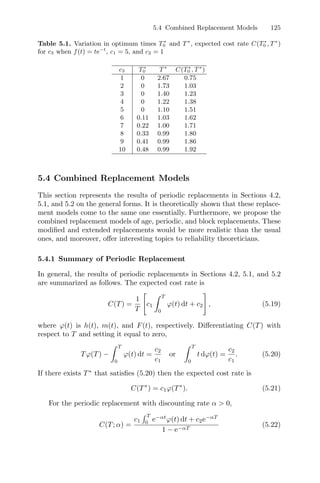
![126 5 Block Replacement
1 − e−αT
α
ϕ(T) −
T
0
e−αt
ϕ(t) dt =
c2
c1
(5.23)
C(T∗
; α) =
c1
α
ϕ(T∗
) − c2. (5.24)
Moreover, the expected cost rate is rewritten on a general form
C(T) =
1
T
[Φ(T) + c2],
where Φ(T) is the total expected cost during (0, T], and the optimum policies
were discussed under several conditions in [29–31]. Furthermore, if the main-
tenance cost depends on time t and is given by c(t), the expected cost rate
is [32]
C(T) =
1
T
# T
0
c(t)ϕ(t) dt + c2
$
.
Finally, we consider a system consisting of n units that operate indepen-
dently of each other and have parameter function ϕi(t) (i = 1, 2, . . . , n). It is
assumed that all units are replaced together at times kT (k = 1, 2, . . . ). Then,
the expected cost rate is
C(T) =
1
T
# n
i=1
ci
T
0
ϕi(t) dt + c2
$
,
where ci = cost of maintenance for each failed unit. Such group maintenance
policies for multiunit systems were analyzed in [33–36], and their overviews
were presented in [37,38].
If the failure rate h(t), renewal density m(t), and failure distribution F(t)
are statistically estimated and graphically drawn, we could derive roughly
optimum replacement T∗
on the horizontal axis and the expected cost rate
C(T∗
)/c1 on the vertical axis from Figures 4.2, 5.2, and 5.4.
5.4.2 Combined Replacement
This section summarizes the combined replacement models of age, periodic,
and block replacements.
(1) Periodic and No Replacement at Failure
We propose the combined model of periodic replacement with minimal repair
at failures in Section 4.2 and no replacement at failure in Section 5.2: A unit
is replaced at planned time T, where T is given by a solution to (4.18) and
minimizes C(T) in (4.16). If a unit fails during (0, T0] (0 ≤ T0 ≤ T) then
it undergoes only minimal repair at failures, whereas if it fails in an interval](https://image.slidesharecdn.com/maintenancetheoryofreliabilityspringerseriesinreliability-240303085250-86c4adaf/85/Maintenance_Theory_of_Reliability_Springer_Series_in_Reliability-pdf-135-320.jpg)
![5.4 Combined Replacement Models 127
(T0, T) then the minimal repair is not made and it remains failed until the
planned time T.
Consider one cycle from time t = 0 to the time that a unit is replaced at
planned time T. Then, the total expected cost in one cycle is given by the
sum of the minimal repair cost during (0, T0], the planned replacement cost,
and the downtime cost when a unit fails in an interval (T0, T). The mean
downtime from a failure to the replacement is
1
F(T0)
T
T0
(T − t) dF(t) = T − T0 −
1
F(T0)
T
T0
F(t) dt.
Thus, from (4.16) in Section 4.2, the expected cost rate is
C(T0; T) =
1
T
c1H(T0) + c2 + c3
#
T − T0 −
1
F(T0)
T
T0
F(t) dt
$
, (5.25)
where c1 = cost of minimal repair at failure, c2 = cost of planned replacement
at time T, and c3 = downtime cost per unit of time from a failure to its
replacement. This is equal to (4.16) when T = T0, and (5.10) when T0 = 0 by
replacing c3 with c1.
We seek an optimum T∗
0 that minimizes C(T0; T) for a fixed T when the
failure rate h(t) is strictly increasing. Differentiating C(T0; T) with respect to
T0 and setting it equal to zero, we have
1
F(T0)
T
T0
F(t) dt =
c1
c3
. (5.26)
It is easy to see that the left-hand side of (5.26) is strictly decreasing in T0
from
T
0
F(t)dt to 0, because h(t) is strictly increasing. Thus, we have the
following optimum policy.
(i) If
T
0
F(t)dt c1/c3 then there exists a finite and unique T∗
0 that satisfies
(5.26). In this case, optimum T∗
0 is an increasing function of T because
the left-hand side of (5.26) is increasing in T.
(ii) If
T
0
F(t)dt ≤ c1/c3 then T∗
0 = 0; i.e., no minimal repair is made.
(2) Periodic and Age Replacements
We consider two combined models of periodic and age replacements and obtain
optimum replacement policies. First, suppose that if a unit fails during (0, T0]
then it undergoes minimal repair at failures. However, if a unit fails in an
interval (T0, T) then it is replaced with a new one before time T, whereas if
it does not fail in an interval (T0, T) then it is replaced at time T.
Because the probability that a unit fails in an interval (T0, T) is [F(T) −
F(T0)]/F(T0), the mean time from T0 to replacement is](https://image.slidesharecdn.com/maintenancetheoryofreliabilityspringerseriesinreliability-240303085250-86c4adaf/85/Maintenance_Theory_of_Reliability_Springer_Series_in_Reliability-pdf-136-320.jpg)
![128 5 Block Replacement
1
F(T0)
#
(T − T0)F(T) +
T
T0
(t − T0) dF(t)
$
=
1
F(T0)
T
T0
F(t) dt
and the expected cost rate is
C(T0, T) =
c1H(T0) + c2 + c3[F(T) − F(T0)]/F(T0)
T0 +
T
T0
F(t) dt/F(T0)
, (5.27)
where c1 and c2 are given in (5.25) and c3 = additional cost of no planned
replacement at failure. This corresponds to periodic replacement in Section 4.2
when T0 = T, and age replacement in Section 3.1 when T0 = 0.
We seek an optimum T∗
0 that minimizes C(T0; T), where a finite T satisfies
(4.18) when h(t) is strictly increasing. Differentiating C(T0, T) in (5.27) with
respect to T0 and setting it equal to zero,
Q1(T0; T) = c2 + c3 − c1, (5.28)
where
Q1(T0; T) ≡
T0
T
T0
F(t) dt
[c1F(T0) − c3F(T)] − c1H(T0).
Also, we have Q1(0; T) = 0, and differentiating Q1(T0; T) with respect to T0,
dQ1(T0; T)
dT0
=
#
1 +
T0F(T0)
T
T0
F(t) dt
$#
c1F(T0) − c3F(T)
T
T0
F(t) dt
− c1h(T0)
$
.
First, suppose that c3 ≥ c1. Then, Q1(0; T) c2 + c3 − c1, limT0→T
Q1(T0; T) = −∞ for c3 c1 and limT0→T Q1(T0; T) = c2 for c3 = c1. Fur-
thermore, putting dQ1(T0; T)/dT0 = 0 and arranging it, we have
h(T0)
T
T0
F(t) dt − F(T0) = −
c3
c1
F(T). (5.29)
Thus, if c3F(T) ≥ c1[1−h(0)
T
0
F(t)dt] then dQ1(T0; T)/dT0 ≤ 0. Conversely,
if c3F(T) c1[1−h(0)
T
0
F(t)dt] then (5.29) has one solution in 0 T0 T,
and its extreme value is
Q1(T0; T) = c1[T0h(T0) − H(T0)] c2
inasmuch as th(t) − H(t) is an increasing function of t and Th(T) − H(T) =
c2/c1. In both cases, Q1(T0; T) ≤ c2 + c3 − c1 for all T0(0 ≤ T0 ≤ T); i.e.,
C(T0; T) is decreasing in T0, and hence, T∗
0 = T.
Next, suppose that c3 c1. Then, Q1(T0; T) is strictly increasing in T0 be-
cause dQ1(T0; T)/dT0 0 from (ii) of Theorem 1.1 and limT0→T Q1(T0; T) =
∞. If c2 + c3 c1 then Q1(0; T) c2 + c3 − c1, and hence, there exists a
unique T∗
0 (0 T∗
0 T) that satisfies (5.28), and it minimizes C(T0; T). On
the other hand, if c2 + c3 ≤ c1 then Q1(0; T) ≥ c2 + c3 − c1. Thus, C(T0; T)
is increasing in T0, and hence, T∗
0 = 0.
From the above discussion, we have the following optimum policy.](https://image.slidesharecdn.com/maintenancetheoryofreliabilityspringerseriesinreliability-240303085250-86c4adaf/85/Maintenance_Theory_of_Reliability_Springer_Series_in_Reliability-pdf-137-320.jpg)
![5.4 Combined Replacement Models 129
(i) If c3 ≥ c1 then T∗
0 = T; i.e., a unit undergoes only minimal repair until
the replacement time comes.
(ii) If c2 + c3 c1 c3 then there exists a unique T∗
0 (0 T∗
0 T) that
satisfies (5.28), and the resulting cost rate is
C(T∗
0 ; T) =
c1F(T∗
0 ) − c3F(T)
T
T ∗
0
F(t) dt
(5.30)
and the expected cost rate is between two costs:
c1h(T∗
0 ) C(T∗
0 ; T) c1h(T).
(iii) If c1 ≥ c2 + c3 then T∗
0 = 0; i.e., a unit is replaced at failure or at time T,
whichever occurs first.
This policy was called the (T0, T) policy, and it was proved that if c2 +c3
c1 c3 and h(t) is strictly increasing to infinity then there exist finite and
unique T∗
0 and T∗
(0 T∗
0 T∗
∞) that minimize C(T0; T) in (5.27) [39].
Some modified models of this policy were proposed in [40–44].
Next, suppose that if a unit fails during (0, T] then it undergoes minimal
repair at failures. However, a unit is not replaced at time T and is replaced
at the first failure after time T or at time T1 (T1 T), whichever occurs first,
where T satisfies (4.18).
Changing T0 and T into T and T1 in (5.27), the expected cost rate is
C(T1; T) =
c1H(T) + c2 + c3[F(T1) − F(T)]/F(T)
T +
T1
T
F(t) dt/F(T)
. (5.31)
This corresponds to periodic replacement when T = T1, and age replacement
when T = 0. We seek an optimum T∗
1 that minimizes C(T1; T) for a fixed T
given in (4.18) when h(t) is strictly increasing. Differentiating C(T1; T) with
respect to T1 and putting it to zero,
Q2(T1; T) =
c1
c3
Th(T), (5.32)
where
Q2(T1; T) ≡ h(T1)
#
T +
T1
T
F(t) dt
F(T)
$
−
F(T1) − F(T)
F(T)
.
From the assumption that h(t) is strictly increasing, Q2(T1; T) is also strictly
increasing with Q2(T; T) = Th(T) and
Q2(∞; T) ≡ lim
T1→∞
Q2(T1; T) = h(∞)
#
T +
∞
T
F(t) dt
F(T)
$
− 1.
Thus, if c3 ≥ c1 then Q2(T; T) ≥ (c1/c3)Th(T), and T∗
1 = T. Conversely, if
c3 c1 and h(∞) K(T) then Q2(T; T) (c1/c3)Th(T) Q2(∞; T), where](https://image.slidesharecdn.com/maintenancetheoryofreliabilityspringerseriesinreliability-240303085250-86c4adaf/85/Maintenance_Theory_of_Reliability_Springer_Series_in_Reliability-pdf-138-320.jpg)
![130 5 Block Replacement
K(T) ≡
(c1/c3)Th(T) + 1
T +
∞
T
F(t) dt/F(T)
.
Hence, there exists a finite and unique T∗
1 that satisfies (5.32), and it min-
imizes C(T1; T). Finally, if c3 c1 and h(∞) ≤ K(T) then Q2(∞; T) ≤
(c1/c3)Th(T), and T∗
1 = ∞.
Therefore, we have the following optimum policy.
(i) If c1 ≤ c3 then T∗
1 = T; i.e., a unit is replaced only at time T.
(ii) If c1 c3 and h(∞) K(T) then there exists a finite and unique T∗
1
(T T∗
1 ∞) that satisfies (5.32) and the resulting cost rate is
C(T∗
1 ; T) = c3h(T∗
1 ). (5.33)
(iii) If c1 c3 and h(∞) ≤ K(T) then T∗
1 = ∞; i.e., a unit is replaced at the
first failure after time T, and the expected cost rate is C(∞; T) = c3K(T).
We compare C(T0; T) and C(T1; T) when c2 + c3 c1 c3 and h(∞)
K(T). From (5.30) and (5.33), if
c1
c3
1
F(T∗
0 )
#
F(T) + h(T∗
1 )
T
T ∗
0
F(t) dt
$
then the replacement after time T is better than the replacement before time
T; i.e., a unit should be replaced late rather than early, and vice versa.
We consider the cases of T1 = ∞ and c3 = 0; i.e., a unit undergoes
minimal repair at failures until time T, and after that, it is replaced at the
first failure [45]. In this case, the expected cost rate is, from (5.31),
C(T) ≡ lim
T1→∞
C(T1; T) =
c1H(T) + c2
T +
∞
T
F(t) dt/F(T)
. (5.34)
By a similar method to the previous models, we have the following results.
(i) If c1 ≥ c2 then T∗
= 0; i.e., a unit is replaced at each failure.
(ii) If c1 c2 and Q3(∞) (c2 − c1)/c1 then there exists a finite and unique
T∗
that satisfies
Q3(T) =
c2 − c1
c1
, (5.35)
where
Q3(T) ≡
TF(T)
∞
T
F(t) dt
− H(T)
and the expected cost rate is
C(T∗
) =
c1F(T∗
)
∞
T ∗ F(t) dt
. (5.36)](https://image.slidesharecdn.com/maintenancetheoryofreliabilityspringerseriesinreliability-240303085250-86c4adaf/85/Maintenance_Theory_of_Reliability_Springer_Series_in_Reliability-pdf-139-320.jpg)
![5.4 Combined Replacement Models 131
(iii) If c1 c2 and Q3(∞) ≤ (c2 − c1)/c1 then T∗
= ∞; i.e., a unit undergoes
only minimal repair at any failure.
Note that when the failure rate h(t) is strictly increasing, Q3(T) is also strictly
increasing and
TF(T)
∞
T
F(t) dt
− H(T) Th(T) − H(T) ≥ T1h(T) − H(T1)
for any T ≥ T1. Thus, if h(t) is strictly increasing to infinity then Q3(∞) = ∞
and there exists a finite and unique T∗
that satisfies (5.35).
(3) Block and Age Replacement
We consider two combined models of block and age replacements. First, sup-
pose that if a unit fails during (0, T0] then it is replaced at each failure. How-
ever, if a unit fails in an interval (T0, T) then it is replaced with a new one
before time T, whereas if it does not fail in (T0, T) then it is replaced at time
T.
From (5.13) in Section 5.3, the probability that a unit fails in an interval
(T0, T) is
G(T − T0; T0) = F(T) −
T0
0
F(T − t) dM(t)
and the mean time to replacement after time T0 is
T −T0
0
(t + T0) dG(t; T0) + TG(T − T0; T0) = T0 +
T −T0
0
G(t; T0) dt.
Thus, the expected cost rate is
C(T0; T) =
c1M(T0) + c2 + c3G(T − T0; T0)
T0 +
T −T0
0
G(t; T0) dt
. (5.37)
This corresponds to age replacement when T0 = 0 and block replacement
when T = T0.
Next, suppose that if a unit fails during (0, T] then it is replaced at each
failure. However, a unit is not replaced at time T, and is replaced at the first
failure after time T or at time T1 (T1 ≥ T), whichever occurs first. Then,
changing T0 and T into T and T1 in (5.37), the expected cost rate is
C(T1; T) =
c1M(T) + c2 + c3G(T1 − T; T)
T +
T1−T
0
G(t; T) dt
. (5.38)
This corresponds to age replacement when T = 0 and block replacement when
T1 = T.
Moreover, if a unit is replaced at the first failure after time T and c3 = 0,
the expected cost rate is
C(T) ≡ lim
T1→∞
C(T1; T) =
c1M(T) + c2
T +
∞
T
F(t) dt +
T
0
[
∞
T −t
F(u) du] dM(t)
. (5.39)](https://image.slidesharecdn.com/maintenancetheoryofreliabilityspringerseriesinreliability-240303085250-86c4adaf/85/Maintenance_Theory_of_Reliability_Springer_Series_in_Reliability-pdf-140-320.jpg)
![132 5 Block Replacement
(4) Block and Periodic Replacements
A unit is replaced at each failure during (0, T0] and at planned time T (T0 ≤
T). However, if a unit fails in an interval (T0, T) then it undergoes minimal
repair. Then, from (1.28) in Section 1.3, the expected number of failures in
(T0, T) is
T0
0
[H(T − t) − H(T0 − t)] dPr{δ(T0) ≤ T0 − t}
= F(T0)[H(T) − H(T0)] +
T0
0
[H(T − t) − H(T0 − t)]F(T0 − t) dM(t),
where δ(t) = age of a unit at time t in a renewal process. Thus, the expected
cost rate is
C(T0; T) =
1
T
#
c1M(T0) + c2 + c3{F(T0)[H(T) − H(T0)]
+
T0
0
[H(T − t) − H(T0 − t)]F(T0 − t) dM(t)}
$
, (5.40)
where c1 = cost of replacement at failure, c2 = cost of planned replacement
at time T, and c3 = cost of minimal repair. This corresponds to periodic
replacement when T0 = 0 and block replacement when T = T0.
References
1. Barlow RE and Proschan F (1965) Mathematical Theory of Reliability. J Wiley
Sons, New York.
2. Schweitzer PJ (1967) Optimal replacement policies for hyperexponentially and
uniformly distributed lifetimes. Oper Res 15:360–362.
3. Marathe VP, Nair KPK (1966) Multistage planned replacement strategies. Oper
Res 14:874–887.
4. Jain A, Nair KPK (1974) Comparison of replacement strategies for items that
fail. IEEE Trans Reliab R-23:247–251.
5. Tilquin C, Cléroux R (1975) Block replacement policies with general cost struc-
tures. Technometrics 17:291–298.
6. Archibald TW, Dekker R (1996) Modified block-replacement for multi-
component systems. IEEE Trans Reliab R-45:75–83.
7. Sheu SH (1991) A generalized block replacement policy with minimal repair and
general random repair costs for a multi-unit system. J Oper Res Soc 42:331–341.
8. Sheu SH (1994) Extended block replacement policy with used item and general
random minimal repair cost. Eur J Oper Res 79:405–416.
9. Sheu SH (1996) A modified block replacement policy with two variables and
general random repair cost. J Appl Prob 33:557–572.
10. Sheu SH (1999) Extended optimal replacement model for deteriorating systems.
Eur J Oper Res 112:503–516.
11. Scarf PA, Deara M (2003) Block replacement policies for a two-component sys-
tem with failure dependence. Nav Res Logist 50:70–87.](https://image.slidesharecdn.com/maintenancetheoryofreliabilityspringerseriesinreliability-240303085250-86c4adaf/85/Maintenance_Theory_of_Reliability_Springer_Series_in_Reliability-pdf-141-320.jpg)


![6
Preventive Maintenance
An operating unit is repaired or replaced when it fails. If a failed unit under-
goes repair, it needs a repair time which may not be negligible. After the repair
completion, a unit begins to operate again. If a failed unit cannot be repaired
and spare units are not on hand, it takes a replacement time that might not
be negligible. A unit forms an alternating renewal process that repeats up and
down states alternately in Section 1.3.2. Some reliability quantities such as
availabilities, expected number of failures, and repair limit times have already
been derived in Chapter 2.
When a unit is repaired after failure, i.e., corrective maintenance is done,
it may require much time and high cost. In particular, the downtime of such
systems as computers, plants, and radar should be made as short as possible
by decreasing the number of system failures. In this case, to maintain a unit
to prevent failures, we need to do preventive maintenance (PM), but not to
do it too often from the viewpoints of reliability and cost.
The optimum PM policy that maximizes the availability was first derived
in [1]. Optimum PM policies for more general systems were discussed in [2–6].
The PM policies for series systems by modifying the opportunistic replacement
[7] and for a system with spare units [8, 9] were studied. The PM model
where the failure distribution is uncertain was considered in [10]. Furthermore,
several maintenance models in Europe were presented and a good survey of
applied PM models was given in [11]. The PM programs of plants and aircraft
were given in [12–15]. Several imperfect PM policies where a unit may not be
new at PM are discussed in Chapter 7.
In this chapter, we summarize appropriate PM policies that are suitable
for some systems: In Section 6.1, we consider the PM of a one-unit system and
obtain the reliability quantities such as renewal functions and transition prob-
abilities [2]. Using these results, we derive optimum PM policies that maximize
the availabilities, the expected earning rate, and the interval reliability [16]. In
Section 6.2, we consider the PM of a two-unit standby system and analytically
derive optimum policies that maximize the mean time to system failure and
the availability [17–19]. In Section 6.3, we propose the modified PM policy
135](https://image.slidesharecdn.com/maintenancetheoryofreliabilityspringerseriesinreliability-240303085250-86c4adaf/85/Maintenance_Theory_of_Reliability_Springer_Series_in_Reliability-pdf-144-320.jpg)
![136 6 Preventive Maintenance
which is planned at periodic times, and when the total number of failures has
exceeded a specified number, the PM is done at the next planned time [20].
This is applied to the analysis of restarts for a computer system, the number
of uses, the number of shocks for a cumulative damage model, and the number
of unit failures for a parallel system.
6.1 One-Unit System with Repair
Consider a one-unit system. When a unit fails, it undergoes repair immedi-
ately, and once repaired, it is returned to the operating state. It is assumed
that the failure distribution of a unit is a general distribution F(t) with finite
mean µ ≡
∞
0
F(t)dt, where F ≡ 1 − F, and the repair distribution G1(t) is
also a general distribution with finite mean β1.
We discuss a preventive maintenance policy for a one-unit system with
repair. When a unit operates for a planned time T (0 T ≤ ∞) without
failure, we stop its operation for PM. The distribution of time to the PM
completion is assumed to be a general distribution G2(t) with finite mean β2,
which may be different from the repair distribution G1(t).
It was pointed out [2] that the optimum PM policy maximizing the avail-
ability of the system is reduced to the standard age replacement problem as
described in Section 3.1 if the mean time β1 to repair is replaced with the
replacement cost c1 of a failed unit and the mean time β2 to PM with the
cost c2 of exchanging a nonfailed unit.
6.1.1 Reliability Quantities
We derive renewal functions and transition probabilities of a one-unit system
with repair and PM, using the same regeneration-point techniques found in
Section 1.3.3 on Markov renewal processes. The expected number of system
failures and the availability are easily given by these functions and probabili-
ties, respectively.
To analyze the above system, we define the following system states.
State 0: Unit is operating.
State 1: Unit is under repair.
State 2: Unit is under PM.
These system states represent the continuous states of the system and the
system makes a Markov renewal process (see Figure 6.1). We can obtain re-
newal functions and transition probabilities by using the same techniques as
those in Section 1.3.
Let Mij(t) (i, j = 0, 1, 2) be the expected number of visits to state j
during (0, t], starting from state i. For instance, M02(t) represents the expected
number of exchanges of nonfailed units during (0, t], given that a unit began
to operate at time 0.](https://image.slidesharecdn.com/maintenancetheoryofreliabilityspringerseriesinreliability-240303085250-86c4adaf/85/Maintenance_Theory_of_Reliability_Springer_Series_in_Reliability-pdf-145-320.jpg)
![6.1 One-Unit System with Repair 137
1
2
0
Fig. 6.1. Process of one-unit system
For convenience, we define D(t) as the distribution of a degenerate random
variable placing unit mass at T (0 T ≤ ∞); i.e., D(t) ≡ 0 for t T and 1
for t ≥ T. Then, by considering the transitions between the system states, we
have the following renewal-type equations of Mij(t).
M00(t) =
t
0
D(u) dF(u) ∗ M10(t) +
t
0
F(u) dD(u) ∗ M20(t)
M01(t) =
t
0
D(u) dF(u) ∗ [1 + M11(t)] +
t
0
F(u) dD(u) ∗ M21(t)
M02(t) =
t
0
D(u) dF(u) ∗ M12(t) +
t
0
F(u) dD(u) ∗ [1 + M22(t)]
Mi0(t) = Gi(t) ∗ [1 + M00(t)] (i = 1, 2)
M1j(t) = G1(t) ∗ M0j(t), M2j(t) = G2(t) ∗ M0j(t) (j = 1, 2),
where the asterisk represents the Stieltjes convolution; i.e., a(t) ∗ b(t) ≡
t
0
b(t − u)da(u) for any a(t) and b(t), and Ψ ≡ 1 − Ψ for any distribution Ψ.
Let Ψ∗
(s) be the Laplace–Stieltjes (LS) transform of any function Ψ(t);
i.e., Ψ∗
(s) ≡
∞
0
e−st
dΨ(t) for s 0. Forming the LS transforms of the above
equations, we have
M∗
00(s) =
T
0
e−st
dF(t)M∗
10(s) + e−sT
F(T)M∗
20(s)
M∗
01(s) =
T
0
e−st
dF(t)[1 + M∗
11(s)] + e−sT
F(T)M∗
21(s)
M∗
02(s) =
T
0
e−st
dF(t)M∗
12(s) + e−sT
F(T)[1 + M∗
22(s)]
M∗
i0(s) = G∗
i (s)[1 + M∗
00(s)] (i = 1, 2)
M∗
1j(s) = G∗
1(s)M∗
0j(s), M∗
2j(s) = G∗
2(s)M∗
0j(s) (j = 1, 2).
Thus, solving the equations for M∗
0j(s) (j = 0, 1, 2), we have](https://image.slidesharecdn.com/maintenancetheoryofreliabilityspringerseriesinreliability-240303085250-86c4adaf/85/Maintenance_Theory_of_Reliability_Springer_Series_in_Reliability-pdf-146-320.jpg)
![138 6 Preventive Maintenance
M∗
00(s) =
G∗
1(s)
T
0
e−st
dF(t) + G∗
2(s)e−sT
F(T)
1 − G∗
1(s)
T
0
e−st dF(t) − G∗
2(s)e−sT F(T)
(6.1)
M∗
01(s) =
T
0
e−st
dF(t)
1 − G∗
1(s)
T
0
e−st dF(t) − G∗
2(s)e−sT F(T)
(6.2)
M∗
02(s) =
e−sT
F(T)
1 − G∗
1(s)
T
0
e−st dF(t) − G∗
2(s)e−sT F(T)
. (6.3)
Furthermore, from (1.63), the limiting values Mj ≡ limt→∞ M0j(t)/t =
lims→0 sM∗
0j(s); i.e., the expected numbers of visits to state j per unit of
time in the steady-state are
M0 =
1
T
0
F(t) dt + β1F(T) + β2F(T)
(6.4)
M1 =
F(T)
T
0
F(t) dt + β1F(T) + β2F(T)
(6.5)
M2 =
F(T)
T
0
F(t) dt + β1F(T) + β2F(T)
. (6.6)
Next, let Pij(t) (i, j = 0, 1, 2) be the transition probability that the system
is in state j at time t, starting from state i at time 0. Then, in a similar way,
we have the following renewal equations of the transition probabilities.
P00(t) = F(t)D(t) +
t
0
D(u) dF(u) ∗ P10(t) +
t
0
F(u) dD(u) ∗ P20(t)
P0j(t) =
t
0
D(u) dF(u) ∗ P1j(t) +
t
0
F(u) dD(u) ∗ P2j(t) (j = 1, 2)
Pi0(t) = Gi(t) ∗ P00(t) (i = 1, 2)
Pjj(t) = Gj(t) + Gj(t) ∗ P0j(t) (j = 1, 2)
P12(t) = G1(t) ∗ P02(t), P21(t) = G2(t) ∗ P01(t).
Thus, forming the LS transforms and solving them for P∗
0j(s) (j = 0, 1, 2),
P∗
00(s) =
1 −
T
0
e−st
dF(t) − e−sT
F(T)
1 − G∗
1(s)
T
0
e−st dF(t) − G∗
2(s)e−sT F(T)
(6.7)
P∗
01(s) =
[1 − G∗
1(s)]
T
0
e−st
dF(t)
1 − G∗
1(s)
T
0
e−st dF(t) − G∗
2(s)e−sT F(T)
(6.8)
P∗
02(s) =
[1 − G∗
2(s)]e−sT
F(T)
1 − G∗
1(s)
T
0
e−st dF(t) − G∗
2(s)e−sT F(T)
. (6.9)
Furthermore, the limiting probabilities Pj ≡ limt→∞ Pij(t) = lims→0 P∗
ij(s)
are](https://image.slidesharecdn.com/maintenancetheoryofreliabilityspringerseriesinreliability-240303085250-86c4adaf/85/Maintenance_Theory_of_Reliability_Springer_Series_in_Reliability-pdf-147-320.jpg)
![6.1 One-Unit System with Repair 139
P0 =
T
0
F(t) dt
T
0
F(t) dt + β1F(T) + β2F(T)
(6.10)
P1 =
β1F(T)
T
0
F(t) dt + β1F(T) + β2F(T)
(6.11)
P2 =
β2F(T)
T
0
F(t) dt + β1F(T) + β2F(T)
, (6.12)
where P0 + P1 + P2 = 1. It is of great interest to have the relation that
Pj = βjMj (j = 1, 2).
Also, note that the probability P00(t) represents the pointwise availability
of the system at time t, given that a unit began to operate at time 0, and
P01(t) + P02(t) is the pointwise unavailability at time t. It is also noted that
the limiting probability P0 represents the steady-state availability, and P1 +P2
is the steady-state unavailability.
6.1.2 Optimum Policies
(1) Availability
We derive an optimum PM time T∗
maximizing the availability P0 that is a
function of T. From (6.10), P0 is rewritten as
P0 = 1
#
1 +
β1F(T) + β2F(T)
T
0
F(t) dt
$
. (6.13)
Thus, the policy maximizing P0 is the same as minimizing the expected cost
rate C(T) in (3.4) by replacing βi with ci (i = 1, 2). We have the same
theorems as those in Section 3.1 under the assumption that β1 β2.
(2) Expected Earning Rate
Introduce the following earnings in specifying the PM policy. Let e0 be a
net earning per unit of time made by the production of an operating unit.
Furthermore, let e1 be an earning rate per unit of time while a unit is under
repair and e2 be an earning rate per unit of time while a unit is under PM.
Both e1 and e2 are usually negative, and may be e0 e2 e1. Then, from
(6.10) to (6.12), the expected earning rate is
E(T) ≡ e0P0 + e1P1 + e2P2 =
e0
T
0
F(t) dt + e1β1F(T) + e2β2F(T)
T
0
F(t) dt + β1F(T) + β2F(T)
.
(6.14)
We can also obtain an optimum policy that maximizes E(T) by a similar
method. If e0 = 0, i.e., we consider no earning of the operating unit, then
E(T) agrees with that of [22, p. 42].](https://image.slidesharecdn.com/maintenancetheoryofreliabilityspringerseriesinreliability-240303085250-86c4adaf/85/Maintenance_Theory_of_Reliability_Springer_Series_in_Reliability-pdf-148-320.jpg)
![140 6 Preventive Maintenance
(3) Emergency Event
Suppose that a unit is required for operation when an emergency event oc-
curs. A typical example of such a model is standby generators in hospitals
or buildings whenever the electric power stops. In any case, it is catastrophic
and dangerous that the unit has failed when an emergency event occurs. We
wish to lessen the probability of such an event by adopting the PM policy.
It is assumed that an emergency event occurs randomly in time; i.e., it
occurs according to an exponential distribution (1 − e−αt
) (0 α ∞) [23].
Then, the probability 1 − A(T) that the unit has failed when an emergency
event occurs is
1 − A(T) =
∞
0
[P01(t) + P02(t)] d(1 − e−αt
)
= P∗
01(α) + P∗
02(α).
Thus, from (6.8) and (6.9), we have
A(T) =
T
0
αe−αt
F(t) dt
1 − G∗
1(α)
T
0
e−αt dF(t) − G∗
2(α)e−αT F(T)
. (6.15)
We can derive an optimum policy that maximizes A(T) by a similar method,
under the assumption that G∗
2(α) G∗
1(α); i.e., the PM rate of a nonfailed
unit is greater than the repair rate of a failed unit.
6.1.3 Interval Reliability
Interval reliability R(x, T0) is defined in Chapter 1 as the probability that at
a specified time T0, a unit is operating and will continue to operate for an
interval of time x. In this section, we consider the case where T0 is distributed
exponentially. A typical model is a standby generator, in which T0 is the time
until the electric power stops and x is the required time until the electric
power recovers. In this case, the interval reliability represents the probability
that a standby generator will be able to operate while the electric power is
interrupted.
Consider a one-unit system that is repaired upon failure and brought back
to operation after the repair completion. The failure time has a general distri-
bution F(t) with finite mean µ and the repair time has a general distribution
G(t) with finite mean β. We set the PM time T (0 T ≤ ∞) for the operating
unit. However, the PM of the operating unit is not done during the interval
[T0, T0 + x] even if it is time for PM. It is assumed that the distribution of
time to the PM completion is the same as the repair distribution G(t).
Similar to (2.28) in Section 2.1, we obtain the interval reliability R(T; x, T0):
R(T; x, T0) = F(T0 + x)D(T0) +
T0
0
F(T0 + x − u)D(T0 − u) dM00(u),](https://image.slidesharecdn.com/maintenancetheoryofreliabilityspringerseriesinreliability-240303085250-86c4adaf/85/Maintenance_Theory_of_Reliability_Springer_Series_in_Reliability-pdf-149-320.jpg)
![6.1 One-Unit System with Repair 141
where M00(t) represents the expected number of occurrences of the recovery
of operating state during (0, t], and its LS transform can be given by putting
G1 = G2 = G in (6.1). Thus, forming the Laplace transform of the above
equation, we have
R∗
(T; x, s) ≡
∞
0
e−sT0
R(T; x, T0) dT0
=
esx
T +x
x
e−st
F(t) dt
1 − G∗(s) + sG∗(s)
T
0
e−stF(t) dt
. (6.16)
Thus, the limiting interval reliability is
R(T; x) ≡ lim
T0→∞
R(T; x, T0) = lim
s→0
sR∗
(T; x, s)
=
T +x
x
F(t) dt
T
0
F(t) dt + β
(6.17)
and the interval reliability when T0 is a random variable with an exponential
distribution (1 − e−αt
) (0 α ∞) is
R(T; x, α) ≡
∞
0
R(T; x, T0) d(1 − e−αT0
) = αR∗
(T; x, α). (6.18)
It is noted that R(T; x) and R(T; x, α)/α agree with (2.30) and (2.29), re-
spectively, in the case of no PM; i.e., T = ∞.
First, we seek an optimum PM time that maximizes the interval reliability
R(T; x) in (6.17) for a fixed x 0. Let λ(t; x) ≡ [F(t + x) − F(t)]/F(t) for
t ≥ 0. Then, both λ(t; x) and h(t) ≡ f(t)/F(t) are called the failure rate and
have the same properties as mentioned in Section 1.1. It is noted that h(t)
has already played an important role in analyzing the replacement models in
Chapters 3 and 4. Let
K1 ≡
x
0
F(t) dt + β
µ + β
= 1 − R(∞; x).
Then, we have the following optimum policy.
Theorem 6.1. Suppose that the failure rate λ(t; x) is continuous and strictly
increasing in t for x 0.
(i) If λ(∞; x) K1 then there exists a finite and unique T∗
(0 T∗
∞)
that satisfies
λ(T; x)
# T
0
F(t) dt + β
$
−
T
0
[F(t) − F(t + x)] dt = β (6.19)
and the resulting interval reliability is
R(T∗
; x) = 1 − λ(T∗
; x). (6.20)](https://image.slidesharecdn.com/maintenancetheoryofreliabilityspringerseriesinreliability-240303085250-86c4adaf/85/Maintenance_Theory_of_Reliability_Springer_Series_in_Reliability-pdf-150-320.jpg)
![142 6 Preventive Maintenance
(ii) If λ(∞; x) ≤ K1 then T∗
= ∞; i.e., no PM is done.
Proof. Differentiating R(T; x) in (6.17) with respect to T and putting it
equal to zero, we have (6.19). Letting Q1(T) be the left-hand side of (6.19),
it is easy to prove that Q1(T) is strictly increasing,
Q1(0) ≡ lim
T →0
Q1(T) = βF(x)
Q1(∞) ≡ lim
T →∞
Q1(T) = λ(∞; x)(µ + β) −
x
0
F(t) dt.
If λ(∞; x) K1 then Q1(∞) β Q1(0). Thus, from the monotonicity and
the continuity of Q1(T), there exists a finite and unique T∗
that satisfies (6.19)
and maximizes R(T; x). Furthermore, from (6.19), we clearly have (6.20).
If λ(∞; x) ≤ K1 then Q1(∞) ≤ β; i.e., R(T; x) is strictly increasing. Thus,
the optimum PM time is T∗
= ∞.
It is of interest that 1 − λ(T∗
; x) in (6.20) represents the probability that
a unit with age T∗
does not fail in a finite interval (T∗
, T∗
+ x].
In the case (i) of Theorem 6.1, we can get the following upper limit of the
optimum PM time T∗
.
Theorem 6.2. Suppose that the failure rate λ(t; x) is continuous and strictly
increasing, λ(0; x) K1 λ(∞; x). Then, there exists a finite and unique T
that satisfies λ(T; x) = K1 and T∗
T.
Proof. From the assumption that λ(t; x) is strictly increasing, we have
λ(T; x)
∞
T
[F(t) − F(t + x)] dt
∞
T
F(t) dt
for 0 ≤ T ∞.
Thus, we have the inequality
Q1(T) λ(T; x)(µ + β) −
x
0
F(t) dt for 0 ≤ T ∞.
Therefore, if there exists T that satisfies
λ(T; x)(µ + β) −
x
0
F(t) dt = β,
i.e., λ(T; x) = K1, then T∗
T. It can be seen that T is finite and unique
inasmuch as λ(T; x) is strictly increasing, and λ(0; x) K1 λ(∞; x). If
λ(0; x) ≥ K1 then we may take T = ∞.
If the time for PM has a distribution G2(t) with mean β2 and the time
for repair has a distribution G1(t) with mean β1, then the limiting interval
reliability is given by](https://image.slidesharecdn.com/maintenancetheoryofreliabilityspringerseriesinreliability-240303085250-86c4adaf/85/Maintenance_Theory_of_Reliability_Springer_Series_in_Reliability-pdf-151-320.jpg)
![6.1 One-Unit System with Repair 143
R(T; x) =
T +x
x
F(t) dt
T
0
F(t) dt + β1F(T) + β2F(T)
. (6.21)
Next, we consider the optimum PM policy that maximizes the interval
reliability when T0 is distributed exponentially. From (6.16) and (6.18),
R(T; x, α) =
αeαx
T +x
x
e−αt
F(t) dt
αG∗(α)
T
0
e−αtF(t) dt + 1 − G∗(α)
. (6.22)
Let
K2(α) ≡
1 − F∗
(α)G∗
(α) − αG∗
(α)eαx
∞
x
e−αt
F(t) dt
1 − F∗(α)G∗(α)
= 1−G∗
(α)R(∞; x, α).
Then, in similar ways to those of obtaining Theorems 6.1 and 6.2, we can get
the following theorems without proof.
Theorem 6.3. Suppose that the failure rate λ(t; x) is continuous and strictly
increasing.
(i) If λ(∞; x) K2(α) then there exists a finite and unique T∗
(0 T∗
∞)
that satisfies
λ(T; x)
#
1 − G∗
(α) + αG∗
(α)
T
0
e−αt
F(t) dt
$
− αG∗
(α)
T
0
e−αt
[F(t) − F(t + x)] dt = 1 − G∗
(α) (6.23)
and the resulting interval reliability is
R(T∗
; x, α) =
1
G∗(α)
[1 − λ(T∗
; x)]. (6.24)
(ii) If λ(∞; x) ≤ K2(α) then T∗
= ∞.
Theorem 6.4. Suppose that the failure rate λ(t; x) is continuous and strictly
increasing, λ(0; x) K2(α) λ(∞; x). Then, there exists a finite and unique
T that satisfies λ(T; x) = K2(α), and T∗
T.
Example 6.1. We compute the PM time T∗
that maximizes the limiting
interval reliability R(T; x) in (6.17) numerically when F(t) = 1−(1+λt)e−λt
;
that is,
λ(t; x) = 1 −
1 +
λx
1 + λt
e−λx
K1 =
(2/λ)(1 − e−λx
) − xe−λx
+ β
2/λ + β
.](https://image.slidesharecdn.com/maintenancetheoryofreliabilityspringerseriesinreliability-240303085250-86c4adaf/85/Maintenance_Theory_of_Reliability_Springer_Series_in_Reliability-pdf-152-320.jpg)
![144 6 Preventive Maintenance
Table 6.1. Dependence of interval of time x in the optimum time T ∗
, the upper
bound T , the interval reliabilities R(T ∗
; x) and R(∞; x) when β = 1 and 2/λ = 10
x T ∗
T R(T ∗
; x) R(∞; x)
1 ∞ ∞ 0.819 0.819
2 16.64 17.00 0.732 0.731
3 10.60 11.50 0.654 0.649
4 8.43 9.66 0.583 0.572
5 7.30 8.75 0.517 0.502
6 6.60 8.20 0.457 0.438
7 6.12 7.83 0.402 0.381
8 5.77 7.57 0.352 0.330
9 5.50 7.38 0.307 0.286
10 5.30 7.22 0.267 0.246
11 5.13 7.10 0.231 0.211
The failure rate λ(t; x) is strictly increasing with λ(0; x) ≡ F(x) and λ(∞; x) =
1 − e−λx
. From (i) of Theorem 6.1, if x ≤ β then we should do no PM of the
operating unit. Otherwise, the optimum time T∗
is a unique solution of the
equation
λT(x − β) − x(1 − e−λT
) = (1 + λx)β
and
R(T∗
; x) =
1 +
λx
1 + λT∗
e−λx
.
From Theorem 6.2, we have the upper limit T of T∗
:
λT∗
x + (λx + 1)β
x − β
.
Table 6.1 presents T∗
, R(T∗
; x), R(∞; x), and T for x = 1, 2, . . . , 11 when
µ = 2/λ = 10 and β = 1.
6.2 Two-Unit System with Repair
We discuss a system that consists of one operating unit with one standby unit,
where the repair and PM are considered. Such a system is called a two-unit
standby redundant system with repair and PM. Two PM policies, strict PM
and slide PM were considered and the method of approximating the optimum
PM policy that maximizes the mean time to system failure (MTTF) was
obtained in [24]. It was shown in [25] that the MTTF of the same system with
PM is greater than that of a similar system with only repair maintenance.](https://image.slidesharecdn.com/maintenancetheoryofreliabilityspringerseriesinreliability-240303085250-86c4adaf/85/Maintenance_Theory_of_Reliability_Springer_Series_in_Reliability-pdf-153-320.jpg)
![6.2 Two-Unit System with Repair 145
The replacement of a two-unit system was considered in [26–28], where at
the failure points of one unit, the other unit is replaced if its age exceeds a
control limit. The maintenance strategy for a two-unit standby system with
waiting time for repair was obtained in [29]. The opportunistic replacement
policies for two-unit systems [30,31] and imperfectly monitored two-unit par-
allel systems [32] were examined. The early results of two-unit systems were
extensively surveyed in [33].
We adopt a slide PM policy which is explained below, and derive optimum
PM policies that maximize the MTTF and the availability. It is noted that in
this section, the availability refers to the steady-state availability.
6.2.1 Reliability Quantities
Consider a standby redundant system that consists of two identical units. The
failure time of an operating unit has a general distribution F(t) with finite
mean µ, and its repair time also has a general distribution G1(t) with finite
mean β1. When an operating unit fails and the other unit is in standby state,
a failed unit undergoes repair immediately and a standby unit takes over its
operation. However, when an operating unit fails while the other unit is still
under repair, a new failed unit has to wait until a failed unit under repair is
completed by a repairperson. This situation means system failure.
It is assumed that a failed unit recovers its functioning as good as new
upon the repair completion, and that a standby unit neither deteriorates nor
fails during the standby interval. Furthermore, each switchover is perfect and
instantaneous, where each switchover is made when an operating unit fails,
a failed unit undergoes repair, and the other standby unit takes over its op-
eration. Two units are alternately used for its operation as described above.
Even if system failure occurs, the system can operate again upon the repair
completion. Thus, the system assumes up and down states repeatedly.
Next, we adopt the same PM policy as in Section 6.1. When a unit operates
for a planned time T (0 ≤ T ≤ ∞) without failure, we stop the operation of a
working unit for PM. It is assumed that the time to the PM completion has a
general distribution G2(t) with finite mean β2, and after PM, a unit recovers
its operation as good as new.
Also, the following two assumptions are made.
(1) The PM of an operating unit is done only if the other unit is on standby.
(2) An operating unit, which forfeited the PM due to assumption (1), un-
dergoes PM just upon the repair completion of a failed unit or the PM
completion.
Assumption (1) can be thought of as avoiding the situation when the PM of
an operating unit causes system failure. Another reason is that the PM of an
operating unit can be done only when a repairperson is free. However, if we
make only assumption (1), an operating unit, which forfeited the PM because
of assumption (1), undergoes no PM forever. This contradicts the concept of](https://image.slidesharecdn.com/maintenancetheoryofreliabilityspringerseriesinreliability-240303085250-86c4adaf/85/Maintenance_Theory_of_Reliability_Springer_Series_in_Reliability-pdf-154-320.jpg)


![148 6 Preventive Maintenance
(1) First-Passage Time Distribution
We derive the first-passage time distribution to system failure and its MTTF,
using the above mass functions. Let Fij(t) (i = −1, 1, 2; j = 1, 2, 3) denote
the first-passage time distribution from the epoch for state i to the epoch for
state j.
First, consider the first-passage time distribution Fij(t) (i, j = 1, 2). Recall
that the epochs for States 1 and 2 are the regeneration points, but the epochs
for States 0 and 3 are not. Then, from the renewal-theoretic arguments,
Fi1(t) = Q
(0)
i1 (t) + Q
(3)
i1 (t) + Q
(0)
i2 (t) ∗ F21(t) (i = 1, 2)
Fi2(t) = Q
(0)
i2 (t) + [Q
(0)
i1 (t) + Q
(3)
i1 (t)] ∗ F12(t) (i = 1, 2),
where the asterisk denotes the Stieltjes convolution.
Next, consider the first-passage time distribution Fi3(t) (i = 1, 2). Then,
we have the following renewal-type equation.
Fi3(t) = Qi3(t) + Q
(0)
i1 (t) ∗ F13(t) + Q
(0)
i2 (t) ∗ F23(t) (i = 1, 2).
If the system starts from State −1 then
F−13(t) = Q−11(t) ∗ F13(t) + Q−12(t) ∗ F23(t).
Taking the LS transform of the above equations and solving them for F∗
−13(s),
we have
F∗
−13(s) =
Q∗
−11(s){Q∗
13(s)[1 − Q
∗(0)
22 (s)] + Q
∗(0)
12 (s)Q∗
23(s)}
+ Q∗
−12(s){Q∗
23(s)[1 − Q
∗(0)
11 (s)] + Q
∗(0)
21 Q∗
13(s)}
[1 − Q
∗(0)
22 (s)][1 − Q
∗(0)
11 (s)] − Q
∗(0)
12 (s)Q
∗(0)
21 (s)
(6.34)
which is the LS transform of the first-passage time distribution to system
failure, starting from State −1.
Therefore, the mean time to system failure is
l−13(T) ≡
∞
0
t dF−13(t) = − lim
s→0
dF∗
−13(s)
ds
= lim
s→0
1 − F∗
−13(s)
s
=
{γ1 +
T
0
[q1 + G1(t)]F(t) dt}
T
0
[q2 + G2(t)] dF(t)
+ {γ2 +
T
0
[q2 + G2(t)]F(t) dt}{1 −
T
0
[q1 + G1(t)] dF(t)}
q1
T
0
[q2 + G2(t)] dF(t) + q2{1 −
T
0
[q1 + G1(t)] dF(t)}
(6.35)
or
l−13(T) =
{µ(1 + q1) −
∞
T
[q1 + G1(t)]F(t) dt}{1 −
∞
T
[q2 + G2(t)] dF(t)}
+ {µ(1 + q2) −
∞
T
[q2 + G2(t)]F(t) dt}
∞
T
[q1 + G1(t)] dF(t)
q1{1 −
∞
T
[q2 + G2(t)] dF(t)} + q2
∞
T
[q1 + G1(t)] dF(t)
,
(6.36)](https://image.slidesharecdn.com/maintenancetheoryofreliabilityspringerseriesinreliability-240303085250-86c4adaf/85/Maintenance_Theory_of_Reliability_Springer_Series_in_Reliability-pdf-157-320.jpg)


![6.2 Two-Unit System with Repair 151
∞
0
L1(t)F(t) dt =
q1γ2 − q2γ1
q1 − q2
.
Differentiating l(T) in (6.35) with respect to T and putting it equal to zero
imply (6.42). Letting the left-hand side of (6.42) be denoted by Q1(T), we
have
dQ1(T)
dT
=
dh(T)
dT
# T
0
L1(t)F(t) dt +
∞
0
L1(t)F(t) dt
$
Q1(0) ≡ lim
T →0
Q1(T) = h(0)
∞
0
L1(t)F(t) dt
Q1(∞) ≡ lim
T →∞
Q1(T) = µh(∞) −
∞
0
L1(t) dF(t).
Thus, if q1γ2 q2γ1 then Q1(T) is continuous and positive for T 0, and is
strictly increasing. Furthermore, let
K0 ≡
q1
∞
0
L1(t) dF(t) + q2
∞
0
L1(t) dF(t)
q1 − q2
0.
If h(0) k1 and h(∞) K1 then Q1(0) K0 Q1(∞). Therefore, there
exists a finite and unique T∗
(0 T∗
∞) that satisfies (6.42), and it
maximizes l(T). If h(0) ≥ k1 then Q1(0) ≥ 0. Thus, l(T) is strictly decreasing
in T, and hence, T∗
= 0. If h(∞) ≤ K1 then Q1(∞) ≤ 0. Thus, l(T) is strictly
increasing in T, and hence, T∗
= ∞; i.e., no PM is done.
On the other hand, if q1γ2 q2γ1 then Q1(0) 0, Q1(0) ≤ 0, and
Q1(∞) 0. Furthermore, it is easy to see that there exists a unique solu-
tion T1 to dQ1(T)/dT = 0 for 0 T ∞, Thus, Q1(T) is a unimodal
function, and hence, Q1(T) is strictly increasing during the interval [T1, ∞).
If q1γ2 = q2γ1 then Q1(0) = 0 and Q1(T) is strictly increasing. In both
cases, i.e., q1γ2 ≤ q2γ1, if h(∞) K1 then there exists a finite and unique T∗
(0 T∗
∞) that satisfies (6.42). Conversely, if h(∞) ≤ K1 then Q1(T) ≤ K0
for any finite T. Thus, the optimum PM time is T∗
= ∞.
By a similar method to that of Theorem 6.4, if there exists T that satisfies
h(T) = K1 then T∗
T.
Next, we derive the optimum PM policy that maximizes the availability.
From (6.39) and (6.40), the availability is given by
A(T) ≡ P0 + P1 + P2
=
[γ1 +
T
0
G1(t)F(t) dt][1 −
∞
T
G2(t) dF(t)]
+ [γ2 +
T
0
G2(t)F(t) dt]
∞
T
G1(t) dF(t)
[β1 +
T
0
G1(t)F(t) dt][1 −
∞
T
G2(t) dF(t)]
+ [β2 +
T
0
G2(t)F(t) dt]
∞
T
G1(t) dF(t)
. (6.43)](https://image.slidesharecdn.com/maintenancetheoryofreliabilityspringerseriesinreliability-240303085250-86c4adaf/85/Maintenance_Theory_of_Reliability_Springer_Series_in_Reliability-pdf-160-320.jpg)
![152 6 Preventive Maintenance
When an operating unit undergoes PM immediately upon the repair or
PM completion, the availability is
A(0) =
q2γ1 + (1 − q1)γ2
q2β1 + (1 − q1)β2
. (6.44)
When no PM is done, the availability is
A(∞) =
µ
µ + β1 − γ1
. (6.45)
Let
ρi ≡
∞
0
Gi(t)F(t) dt = βi − γi (i = 1, 2)
L2(t) ≡
ρ1G2(t) − ρ2G1(t)
ρ1 − ρ2
k2 ≡
ρ1q2 + ρ2(1 − q1)
ρ1β2 − ρ2β1
, K2 ≡
ρ1
µ(ρ1 − ρ2)
.
Theorem 6.6. Suppose that G1(t) G2(t) for 0 t ∞, and the failure
rate h(t) is continuous and strictly increasing.
(i) If h(∞) K2, ρ1β2 ρ2β1, and h(0) k2, or h(∞) K2 and ρ1β2 ≤
ρ2β1, then there exists a finite and unique T∗
(0 T∗
∞) that satisfies
h(T)
# T
0
L2(t)F(t) dt +
∞
0
L2(t) dt
$
−
T
0
L2(t) dF(t)
=
ρ1
∞
0
L2(t) dF(t) + ρ2
∞
0
L2(t) dF(t)
ρ1 − ρ2
. (6.46)
(ii) If h(∞) ≤ K2 then T∗
= ∞; i.e., no PM is done, and the availability is
given in (6.45).
(iii) If ρ1β2 ρ2β1 and h(0) ≥ k2 then T∗
= 0, and the availability is given in
(6.44).
Proof. Differentiating A(T) in (6.43) with respect to T and putting it equal
to zero imply (6.46). In a similar method to that of proving Theorem 6.5, we
can prove this theorem.
By a similar method to that of Theorem 6.4, if there exists T that satisfies
h(T) = K2 then T∗
T.
It has been shown that the problem of maximizing the availability is for-
mally coincident with that of minimizing the expected cost [19].
Example 6.2. We give two numerical problems: to maximize the mean time
to system failure, and to maximize the availability. For the two problems, we](https://image.slidesharecdn.com/maintenancetheoryofreliabilityspringerseriesinreliability-240303085250-86c4adaf/85/Maintenance_Theory_of_Reliability_Springer_Series_in_Reliability-pdf-161-320.jpg)
![6.2 Two-Unit System with Repair 153
assume that Gi(t) = 1 − exp(−θit) (θ2 θ1) and F(t) = 1 − (1 + λt)e−λt
.
It is noted that the failure distribution is a gamma distribution with a shape
parameter 2, and the failure rate h(t) = λ2
t/(1+λt) which is strictly increasing
from 0 to λ.
Consider the first problem of maximizing the mean time to system failure.
Then, we have
qi =
λ
λ + θi
2
(i = 1, 2)
L1(t) =
(λ + θ2)2
e−θ2t
− (λ + θ1)2
e−θ1t
(λ + θ2)2 − (λ + θ1)2
.
From Theorem 6.5, if λ ≤ K1; i.e., (λ + θ2)2
≤ 2(λ + θ1)2
, we should do no
PM of the operating unit. If (λ + θ2)2
2(λ + θ1)2
, we should adopt a finite
and unique PM time T∗
that satisfies
1
1 + λT
{(2λT + e−λT
)[(λ + θ2)2
− (λ + θ1)2
]
−λ2
(e−(λ+θ2)T
− e−(λ+θ1)T
)} = (λ + θ2)2
.
The above equation is derived from (6.42). In this case, the mean time to
system failure is
l(T∗
) =
1
λ4T∗
{(2λT∗
+ e−λT ∗
)[(λ + θ1)2
+ λ2
] − λ2
e−(λ+θ1)T ∗
}.
Furthermore, from the inequality T∗
T, we have
λT∗
(λ + θ2)2
(λ + θ2)2 − 2(λ + θ1)2
which is useful in computing T∗
.
Table 6.2 shows the numerical examples of the dependence of the mean PM
time 1/θ2 in the optimum PM time T∗
and the other quantities when λ = 2
and θ1 = 1. For instance, if θ2 = 8 then T∗
= 0.292, and its associated mean
time is l(T∗
) = 4.447. If we do no PM, i.e., T = ∞, we have l(∞) = 3.250.
Thus, we have [l(T∗
) − l(∞)]/l(∞) × 100% = 36.8% gain in time by adopting
the optimum PM policy.
Let us now consider the second problem of maximizing the availability.
Then, we have
ρi =
λ2
θi(λ + θi)2
(i = 1, 2)
L2(t) =
θ2(λ + θ2)2
e−θ2t
− θ1(λ + θ1)2
e−θ1t
θ2(λ + θ2)2 − θ1(λ + θ1)2
.](https://image.slidesharecdn.com/maintenancetheoryofreliabilityspringerseriesinreliability-240303085250-86c4adaf/85/Maintenance_Theory_of_Reliability_Springer_Series_in_Reliability-pdf-162-320.jpg)
![154 6 Preventive Maintenance
Table 6.2. Dependence of the mean PM time 1/θ2 in the optimum time T ∗
when
2/λ = 1 hr, 1/θ1 = 1 hr, and l(∞) = 3.250 hr
θ2 T ∗
l(T ∗
) l(T ∗
)−l(∞)
l(∞)
×100%
3.0 1.750 3.263 0.4
4.0 0.857 3.398 4.6
5.0 0.557 3.618 11.3
6.0 0.435 3.876 19.2
7.0 0.349 4.156 27.9
8.0 0.292 4.447 36.8
9.0 0.251 4.745 46.0
10.0 0.219 5.047 55.3
From Theorem 6.6, if λ ≤ K2, i.e., θ2(λ + θ2)2
≤ 2θ1(λ + θ1)2
, we should do
no PM of the operating unit. If θ2(λ + θ2)2
2θ1(λ + θ1)2
, we should adopt
PM with finite and unique time T∗
that satisfies
1
1 + λT
{(2λT + e−λT
)[θ2(λ + θ2)2
− θ1(λ + θ1)2
]
−λ2
(θ2e−(λ+θ2)T
− θ1e−(λ+θ1)T
)} = θ2(λ + θ2)2
which is derived from (6.46). In this case, the availability is
A(T∗
) =
θ1(λ + θ1)2
(2λT∗
+ e−λT ∗
) − λ2
θ1e−(λ+θ1)T ∗
λ4T∗ + θ1(λ + θ1)2(2λT∗ + e−λT ∗
) − λ2θ1e−(λ+θ1)T ∗ .
Furthermore, from the inequality T∗
T, we have
λT∗
θ2(λ + θ2)2
θ2(λ + θ2)2 − 2θ1(λ + θ1)2
.
Table 6.3 shows the numerical examples of the dependence of the mean
PM time 1/θ2 in the optimum time T∗
and the other quantities when λ = 2
and θ1 = 1.
6.3 Modified Discrete Preventive Maintenance Policies
This section proposes a new preventive maintenance policy which is more
practical in the real world than the usual PM policies [20]. Failures of a unit
occur at a nonhomogeneous Poisson process and the PM is planned at periodic
times kT (k = 1, 2, . . . ) to prevent failures, where T meaning a day, a week, a
month, and so on, is given. If the total number of failures equals or exceeds a
specified number N, the PM should be done only at the next planned time,
and otherwise, no PM would be done; i.e., we postpone PM until more than
N failures have occurred. Of course, we may consider PM as replacement.](https://image.slidesharecdn.com/maintenancetheoryofreliabilityspringerseriesinreliability-240303085250-86c4adaf/85/Maintenance_Theory_of_Reliability_Springer_Series_in_Reliability-pdf-163-320.jpg)
![6.3 Modified Discrete Preventive Maintenance Policies 155
Table 6.3. Dependence of the mean PM time 1/θ2 in the optimum time T ∗
when
2/λ = 1 hr, 1/θ1 = 1 hr, and A(∞) = 0.643
θ2 T ∗
A(T ∗
) A(T ∗
)−A(∞)
A(∞)
×100%
2.0 1.038 0.698 8.5
3.0 0.402 0.729 13.4
4.0 0.257 0.757 17.7
5.0 0.191 0.779 21.2
6.0 0.153 0.797 24.0
7.0 0.128 0.812 26.4
8.0 0.110 0.825 28.4
9.0 0.096 0.837 30.2
10.0 0.086 0.847 31.7
This is a modification of the policy where a unit undergoes replacement at
the number of N failures in Section 4.3, and would be practical in many cases
because the PM is done only when an operating unit is idle. For example, when
T = 6 days, the PM is done at the next Sunday if more than N failures have
occurred from the previous PM to the end of this week. Moreover, this would
be more economical than the usual periodic policy in Section 4.2, inasmuch
as we employ PM only if some failures have occurred.
We derive the expected cost rate of a unit, using the theory of Poisson
processes, and determine an optimum number N∗
of failures before PM that
minimizes the expected cost rate. It is given by a unique solution of the equa-
tion when the intensity function h(t) of a Poisson process is strictly increasing
to infinity. Furthermore, we consider the model where a unit fails with a cer-
tain probability due to faults and the PM is done if more than N faults have
occurred, and discuss an optimum policy. Finally, we suggest three PM models
where the PM is done by counting the number of occurrences of use, shock,
and unit failure.
These models are actually applied to the PM of a computer system: the sys-
tem stops because of intermittent faults of transient failures [34] due to noise,
temperature, power supply variations, and poor electric contacts. The PM
should be done on weekends if more than N faults or failures have occurred.
For similar reasons, these could be applied to equipment with microcomput-
ers such as numerical control motors and machines, and more extensively to
some machines in the factories of manufacturing companies. This policy was
applied to the PM of hard disks [35] and a phased array radar [36].
6.3.1 Number of Failures
Consider a unit that should operate for an infinite time span. It is assumed
that:
(1) Failures occur at a nonhomogeneous Poisson process with an inten-
sity function h(t), and a mean-value function H(t) ≡
t
0
h(u) du rep-](https://image.slidesharecdn.com/maintenancetheoryofreliabilityspringerseriesinreliability-240303085250-86c4adaf/85/Maintenance_Theory_of_Reliability_Springer_Series_in_Reliability-pdf-164-320.jpg)
![156 6 Preventive Maintenance
resents the expected number of failures during (0, t], and pj[H(t)] ≡
{[H(t)]j
/j!}e−H(t)
(j = 0, 1, 2, . . . ) is the probability that j failures ex-
actly occur during (0, t].
(2) The PM is planned at times kT (k = 1, 2, . . . ) where a positive T (0
T ∞) is given. A unit becomes like new by PM; i.e., the time returns
to zero after PM.
(3) If the total number of failures exceeds a specified number N (N =
1, 2, . . . ), the PM is done at the next planned time. Otherwise, a unit
is left as it is.
(4) A unit undergoes minimal repair at each failure in Section 4.1. The repair
and PM times are negligible; i.e., the time considered here is measured
only by the total operating time of a unit.
(5) An intensity function h(t) is continuous and strictly increasing.
The probability that the PM is done at time (k + 1)T (k = 0, 1, 2, . . . ),
because more than N failures have occurred during (0, (k + 1)T] when the
number of failures was less than N until time kT, is
N−1
j=0
pj[H(kT)]
∞
i=N−j
pi[H((k + 1)T) − H(kT)]
=
N−1
j=0
pj[H(kT)] −
N−1
j=0
pj[H(kT)]
N−j−1
i=0
pi[H((k + 1)T) − H(kT)]
=
N−1
j=0
{pj[H(kT)] − pj[H((k + 1)T)]}
because
∞
i=N−j pi[·] = 1 −
N−j−1
i=0 pi[·], and
N−1
j=0 pj(a)
N−j−1
i=0 pi(b) =
N−1
j=0 pj(a+b) by the property of a Poisson process in Section 1.3. Thus, the
mean time to PM is
∞
k=0
[(k + 1)T]
N−1
j=0
{pj[H(kT)] − pj[H((k + 1)T)]}
= T
⎧
⎨
⎩
∞
k=0
(k + 1)
N−1
j=0
pj[H(kT)] −
∞
k=0
(k + 1)
N−1
j=0
pj[H((k + 1)T)]
⎫
⎬
⎭
= T
∞
k=0
N−1
j=0
pj[H(kT)]. (6.47)
Furthermore, the expected number of failures when the PM is done at time
(k + 1)T is](https://image.slidesharecdn.com/maintenancetheoryofreliabilityspringerseriesinreliability-240303085250-86c4adaf/85/Maintenance_Theory_of_Reliability_Springer_Series_in_Reliability-pdf-165-320.jpg)
![6.3 Modified Discrete Preventive Maintenance Policies 157
N−1
j=0
pj[H(kT)]
∞
i=N−j
(i + j)pi[H((k + 1)T) − H(kT)]
=
N−1
j=0
pj[H(kT)]
∞
i=N
ipi−j[H((k + 1)T) − H(kT)].
Exchanging the summations and noting that
(i
j
)
≡ 0 for i j, we can show
that this is equal to
∞
i=N
N−1
j=0
i
i!
i
j
[H(kT)]j
[H((k + 1)T) − H(kT)]i−j
e−H((k+1)T )
=
∞
i=N
i
i!
e−H((k+1)T )
[H((k + 1)T)]i
−
∞
j=N
i
j
[H(kT)]j
[H((k + 1)T) − H(kT)]i−j
= H((k + 1)T)
∞
j=N−1
pj[H((k + 1)T)] − H(kT)
∞
j=N−1
pj[H(kT)]
− [H((k + 1)T) − H(kT)]
∞
j=N
pj[H(kT)].
Using the relation
∞
j=N pj[·] = 1 −
N−1
j=0 pj[·] and summing it over k from
0 to ∞, the expected number of failures, i.e., minimal repairs before PM, is
∞
k=0
[H((k + 1)T) − H(kT)]
N−1
j=0
pj[H(kT)]. (6.48)
Therefore, from Theorem 1.6 in Chapter 1 and (3.3), the expected cost rate
is
C1(N) =
c1
∞
k=0[H((k + 1)T) − H(kT)]
N−1
j=0 pj[H(kT)] + c2
T
∞
k=0
N−1
j=0 pj[H(kT)]
(N = 1, 2, . . . ), (6.49)
where c1 = cost of minimal repair and c2 = cost of planned PM.
We find an optimum number N∗
that minimizes C1(N). Let
q1(N) =
∞
k=0[H((k + 1)T) − H(kT)]pN [H(kT)]
∞
k=0 pN [H(kT)]
(N = 1, 2, . . . ).
Then, we have the following theorem.](https://image.slidesharecdn.com/maintenancetheoryofreliabilityspringerseriesinreliability-240303085250-86c4adaf/85/Maintenance_Theory_of_Reliability_Springer_Series_in_Reliability-pdf-166-320.jpg)
![158 6 Preventive Maintenance
Theorem 6.7. When h(t) is strictly increasing, q1(N) is also strictly in-
creasing and limN→∞ q1(N) = h(∞).
Proof. From the notation of q1(N), we have
q1(N + 1) − q1(N)
=
∞
k=0[H((k + 1)T) − H(kT)]pN+1[H(kT)]
∞
j=0 pN [H(jT)]
−
∞
k=0[H((k + 1)T) − H(kT)]pN [H(kT)]
∞
j=0 pN+1[H(jT)]
∞
k=0 pN+1[H(kT)]
∞
j=0 pN [H(jT)]
.
The numerator on the right-hand side is
1
N +1
⎧
⎨
⎩
∞
k=0
[H((k+1)T)−H(kT)]pN [H(kT)]
∞
j=0
pN [H(jT)][H(kT)−H(jT)]
⎫
⎬
⎭
=
1
N +1
⎧
⎨
⎩
∞
k=0
[H((k+1)T)−H(kT)]pN[H(kT)]
k
j=0
pN[H(jT)][H(kT)−H(jT)]
−
∞
k=0
pN [H(kT)]
k
j=0
[H((j+1)T) − H(jT)]pN [H(jT)][H(kT) − H(jT)]
⎫
⎬
⎭
=
1
N +1
⎧
⎨
⎩
∞
k=0
pN [H(kT)]
k
j=0
pN [H(jT)][H(kT) − H(jT)]
× [H((k + 1)T) − H(kT) − H((j + 1)T) + H(jT)]
0
because h(t) is strictly increasing.
Next, prove that limN→∞ q1(N) = h(∞). We easily obtain q1(N) ≤ h(∞)
for any finite N, and hence, we need only to show that limN→∞ q1(N) ≥ h(∞).
For any positive number n, q1(N) is rewritten as
q1(N) =
n
k=0[H((k + 1)T) − H(kT)]pN [H(kT)]
+
∞
k=n+1[H((k + 1)T) − H(kT)]pN [H(kT)]
n
k=0 pN [H(kT)] +
∞
k=n+1 pN [H(kT)]
≥
h(nT)
1 + {
n
k=0 pN [H(kT)]/
∞
k=n+1 pN [H(kT)]}
and
lim
N→∞
n
k=0 pN [H(kT)]
∞
k=n+1 pN [H(kT)]
≤ lim
N→∞
n
k=0
H(kT)
H((n + 1)T)
N
e[H((n+1)T )−H(nT )]
= 0.](https://image.slidesharecdn.com/maintenancetheoryofreliabilityspringerseriesinreliability-240303085250-86c4adaf/85/Maintenance_Theory_of_Reliability_Springer_Series_in_Reliability-pdf-167-320.jpg)
![6.3 Modified Discrete Preventive Maintenance Policies 159
Therefore,
lim
N→∞
q1(N) ≥ h(n)
which completes the proof, because n is arbitrary.
From Theorem 6.7, it is easy to see that
C1(∞) ≡ lim
N→∞
C1(N) =
c1h(∞)
T
. (6.50)
Thus, if an intensity function h(t) tends to infinity as t → ∞, there exists a
finite N∗
to minimize C1(N).
We derive an optimum number N∗
that minimizes the expected cost rate
C1(N) in (6.49) when h(t) is strictly increasing.
Theorem 6.8. Suppose that h(t) is continuous and strictly increasing.
(i) If L1(∞) c2/c1 then there exists a finite and unique minimum that
satisfies
L1(N) ≥
c2
c1
(N = 1, 2, . . . ) (6.51)
and the resulting expected cost rate is given by
c1q1(N∗
− 1) TC1(N∗
) ≤ c1q1(N∗
), (6.52)
where
L1(N) ≡ q1(N)
∞
k=0
N−1
j=0
pj[H(kT)]
−
∞
k=0
[H((k + 1)T) − H(kT)]
N−1
j=0
pj[H(kT)] (N = 1, 2, . . . ).
(ii) If L1(∞) ≤ c2/c1 then N∗
= ∞; i.e., the PM is not done and the expected
cost rate is given in (6.50).
Proof. Forming the inequality C1(N + 1) ≥ C1(N), we have
c1
∞
k=0
[H((k + 1)T)−H(kT)]
N
j=0
pj[H(kT)]
∞
k=0
N−1
j=0
pj[H(kT)]
−
∞
k=0
[H((k + 1)T)−H(kT)]
N−1
j=0
pj[H(kT)]
∞
k=0
N
j=0
pj[H(kT)]
≥ c2
∞
k=0
pN [H(kT)].](https://image.slidesharecdn.com/maintenancetheoryofreliabilityspringerseriesinreliability-240303085250-86c4adaf/85/Maintenance_Theory_of_Reliability_Springer_Series_in_Reliability-pdf-168-320.jpg)
![160 6 Preventive Maintenance
Dividing both sides by c1
∞
k=0 pN [H(kT)] and arranging them,
q1(N)
∞
k=0
N−1
j=0
pj[H(kT)] −
∞
k=0
[H((k + 1)T) − H(kT)]
N−1
j=0
pj[H(kT)] ≥
c2
c1
which implies (6.51). Furthermore, from Theorem 6.7,
L1(N + 1) − L1(N) = [q1(N + 1) − q1(N)]
∞
k=0
N−1
j=0
pj[H(kT)] 0
and hence, L1(N) is also strictly increasing. Therefore, if L1(∞) c2/c1 then
there exists a finite and unique minimum N∗
that satisfies (6.51), and from
L1(N∗
− 1) c2/c1 and L1(N∗
) ≥ c2/c1, we have (6.52).
Next, we investigate the limit of L1(N). In a similar way to that of proving
Theorem 6.7, we can easily have
q1(N) ≥
∞
k=0[H((k + 1)T) − H(kT)]
N−1
j=1 pj[H(kT)]
∞
k=0
N−1
j=1 pj[H(kT)]
.
Thus,
L1(N) q1(N)
∞
k=0
p0[H(kT)]
−
∞
k=0
[H((k + 1)T) − H(kT)]p0[H(kT)] (N = 2, 3, . . . )
which implies
lim
N→∞
L1(N) ≥ h(∞)
∞
k=0
p0[H(kT)]
−
∞
k=0
[H((k + 1)T) − H(kT)]p0[H(kT)].
Therefore, if h(∞) TC1(1)/c1 then (6.51) has a finite solution in N.
From the above discussion, we can conclude that if h(t) is strictly in-
creasing to infinity, then there exists a unique minimum N∗
such that
L1(N) ≥ c2/c1 and it minimizes C1(N) in (6.49).
6.3.2 Number of Faults
Faults of a unit occur at a nonhomogeneous Poisson process with an intensity
function h(t). A unit stops its operation due to faults and the restart is made](https://image.slidesharecdn.com/maintenancetheoryofreliabilityspringerseriesinreliability-240303085250-86c4adaf/85/Maintenance_Theory_of_Reliability_Springer_Series_in_Reliability-pdf-169-320.jpg)
![6.3 Modified Discrete Preventive Maintenance Policies 161
instantaneously by the detection of these faults. The restart succeeds with
probability α (0 α 1) and the unit returns to a normal condition. On the
other hand, the restart fails with probability β ≡ 1 − α, and the unit needs
repair. Then, if the total number of successes of restart is more than N, the
PM can be done at the next scheduled time. A unit becomes like new by PM
or repair, and the times for faults, restarts, PMs and repairs are negligible.
The other assumptions are the same as those in Section 6.3.1.
Let Fβ(t) be the probability that a unit survives because all restarts are
successful during (0, t]. Then,
Fβ(t) =
∞
j=0
Pr{unit survives to time t | j faults} × Pr{j faults in (0, t]}
=
∞
j=0
αj
pj[H(t)] = e−βH(t)
. (6.53)
Furthermore, the probability that the PM is done at time (k + 1)T (k =
0, 1, 2, . . . ), because more than N restarts have succeeded until (k +1)T when
j (j = 0, 1, 2, . . . , N − 1) successful restarts were made during (0, kT], is
N−1
j=0
αj
pj[H(kT)]
∞
i=N−j
αi
pi[H((k + 1)T) − H(kT)]
=
N−1
j=0
αj
{pj[H(kT)]e−β[H((k+1)T )−H(kT )]
− pj[H((k + 1)T)]}.
Thus, the probability that the PM is done before failure is
∞
k=0
N−1
j=0
αj
{pj[H(kT)]e−β[H((k+1)T )−H(kT )]
− pj[H((k + 1)T)]}
= 1 −
∞
k=0
[Fβ(kT) − Fβ((k + 1)T)]
N−1
j=0
pj[αH(kT)]. (6.54)
Similarly, the probability that a unit undergoes repair before PM is
∞
k=0
N−1
j=0
αj
pj[H(kT)]
∞
i=0
(1 − αi
)pi[H((k + 1)T) − H(kT)]
=
∞
k=0
[Fβ(kT) − Fβ((k + 1)T)]
N−1
j=0
pj[αH(kT)]. (6.55)
It is evident that (6.54) + (6.55) = 1. Similarly, the mean time to PM or
repair is](https://image.slidesharecdn.com/maintenancetheoryofreliabilityspringerseriesinreliability-240303085250-86c4adaf/85/Maintenance_Theory_of_Reliability_Springer_Series_in_Reliability-pdf-170-320.jpg)
![162 6 Preventive Maintenance
∞
k=0
[(k + 1)T]
N−1
j=0
αj
{pj[H(kT)]e−β[H((k+1)T )−H(kT )]
− pj[H((k + 1)T)]}
+
∞
k=0
N−1
j=0
αj
pj[H(kT)]
∞
i=0
αi
β
(k+1)T
kT
tpi[H(t) − H(kT)]h(t) dt
=
∞
k=0
(k+1)T
kT
Fβ(t) dt
N−1
j=0
pj[αH(kT)]. (6.56)
Therefore, if we neglect all costs resulting from restarts then the expected
cost rate is, from (6.54), (6.55), and (6.56),
C2(N) =
(c1 − c2)
∞
k=0[Fβ(kT) − Fβ((k + 1)T)]
N−1
j=0 pj[αH(kT)] + c2
∞
k=0
(k+1)T
kT
Fβ(t) dt
N−1
j=0 pj[αH(kT)]
(N = 1, 2, . . . ), (6.57)
where c1 = cost of repair and c2 = cost of PM.
It is assumed that c1 c2 because the repair cost would be higher than
the PM cost in the actual field, and µβ ≡
∞
0
Fβ(t) dt ∞ is the finite mean
time to need repair. Let
q2(N) ≡
∞
k=0[Fβ(kT) − Fβ((k + 1)T)]pN [αH(kT)]
∞
k=0
(k+1)T
kT
Fβ(t) dt pN [αH(kT)]
(N = 1, 2, . . . ).
Theorem 6.9. When h(t) is strictly increasing, q2(N) is also strictly in-
creasing and limN→∞ q2(N) ≡ βh(∞).
Proof. We use the following notations.
Bk ≡ e−αH(kT )
(k+1)T
kT
Fβ(t) dt (k = 0, 1, 2, . . . )
Ck ≡ e−αH(kT )
[Fβ(kT) − Fβ((k + 1)T)]. (k = 0, 1, 2, . . . ).
Then, q2(N) is written as
q2(N) =
∞
k=0[H(kT)]N
Ck
∞
k=0[H(kT)]N Bk
.
In a similar way to that of Theorem 6.7, it is easy to prove that when h(t) is
strictly increasing,
βh(kT)
Ck
Bk
βh((k + 1)T), q2(N + 1) − q2(N) 0.
Thus, we have](https://image.slidesharecdn.com/maintenancetheoryofreliabilityspringerseriesinreliability-240303085250-86c4adaf/85/Maintenance_Theory_of_Reliability_Springer_Series_in_Reliability-pdf-171-320.jpg)
![6.3 Modified Discrete Preventive Maintenance Policies 163
lim
k→∞
Ck
Bk
= βh(∞)
and for any positive number n,
βh(nT) ≤ lim
N→∞
q2(N) ≤ βh(∞)
which completes the proof.
From this theorem, it is easy to see that
C2(∞) ≡ lim
N→∞
C2(N) =
c1
µβ
. (6.58)
We derive an optimum number N∗
that minimizes C2(N) in (6.57).
Theorem 6.10. Suppose that h(t) is continuous and strictly increasing.
(i) If βµβh(∞) c1/(c1 − c2) then there exists a finite and unique minimum
that satisfies
L2(N) ≥
c2
c1 − c2
(N = 1, 2, . . . ) (6.59)
and the resulting cost rate is
(c1 − c2)q2(N∗
− 1) C2(N∗
) ≤ (c1 − c2)q2(N∗
), (6.60)
where
L2(N) ≡ q2(N)
∞
k=0
(k+1)T
kT
Fβ(t) dt
N−1
j=0
pj[αH(kT)]
−
∞
k=0
[Fβ(kT) − Fβ((k + 1)T)]
N−1
j=0
pj[αH(kT)] (N = 1, 2, . . . ).
(ii) If βµβh(∞) ≤ c1/(c1 − c2) then N∗
= ∞; i.e., we should do no PM, and
C2(∞) is given in (6.58).
Proof. From the inequality C2(N + 1) ≥ C2(N), we have
(c1 − c2)
⎡
⎣
∞
k=0
/
Fβ(kT) − Fβ((k + 1)T)
0 N
j=0
pj[αH(kT)]
×
∞
k=0
(k+1)T
kT
Fβ(t) dt
N−1
j=0
pj[αH(kT)]](https://image.slidesharecdn.com/maintenancetheoryofreliabilityspringerseriesinreliability-240303085250-86c4adaf/85/Maintenance_Theory_of_Reliability_Springer_Series_in_Reliability-pdf-172-320.jpg)
![164 6 Preventive Maintenance
−
∞
k=0
[Fβ(kT) − Fβ((k + 1)T)]
N−1
j=0
pj[αH(kT)]
×
∞
k=0
(k+1)T
kT
Fβ(t) dt
N
j=0
pj[αH(kT)]
⎤
⎦
≥ c2
∞
k=0
(k+1)T
kT
Fβ(t) dt pN [αH(kT)].
Dividing both sides by (c1 − c2)
∞
k=0
(k+1)T
kT
Fβ(t) dt pN [αH(kT)] implies
L2(N) ≥
c2
c1 − c2
.
Using Theorem 6.9,
L2(N + 1) − L2(N)
= [q2(N + 1) − q2(N)]
∞
k=0
(k+1)T
kT
Fβ(t) dt
N
j=0
pj[αH(kT)] 0
lim
N→∞
L2(N) = βµβh(∞) − 1.
Therefore, similar to Theorem 6.8, we have the results of Theorem 6.10.
Example 6.3. A computer system stops at certain faults according to a
Weibull distribution with shape parameter 2; i.e., H(t) = λt2
. The restart
succeeds with probability α and fails with probability β [37]. If the total
number of successes of restarts exceeds a specified number N, the PM can be
done at the next planned time. Then, from Theorem 6.10, there always exists
an optimum number N∗
(1 ≤ N∗
∞) that satisfies (6.59).
Table 6.4 gives N∗
for T = 24 hours, 48 hours, α = 0.8, 0.85, 0.90, 0.95,
and c1/c2 = 1.5, 2.0, 3.0 when 1/λ = 720 hours. Also, the mean time to N
faults is given by
µN ≡
∞
0
tpN−1[H(t)]h(t) dt =
Γ(N + 1
2 )
√
λ
.
For example, when T = 24 and α = 0.9, µN∗ = 133, 84, 52 hours for N∗
= 25,
10, 4 hours, respectively, and on the average, we may employ PM at about
1 time per 6 days, 1 time per 4 days, and 1 time per 3 days for cost rates
c1/c2 = 1.5, 2.0, and 3.0.
Up to now, we have assumed that the times for repairs and PMs are negli-
gible. If the PM and the repair require the mean times θ2 and θ1, respectively,
then the expected cost rate in (6.57) can be rewritten as](https://image.slidesharecdn.com/maintenancetheoryofreliabilityspringerseriesinreliability-240303085250-86c4adaf/85/Maintenance_Theory_of_Reliability_Springer_Series_in_Reliability-pdf-173-320.jpg)
![6.3 Modified Discrete Preventive Maintenance Policies 165
Table 6.4. Optimum number N∗
that minimizes C2(N) when H(t) = λt2
and
1/λ = 720 hours
T = 24 hours T = 48 hours
α c1/c2 c1/c2
1.5 2.0 3.0 1.5 2.0 3.0
0.80 12 5 1 9 5 1
0.85 18 7 3 18 7 1
0.90 25 10 4 21 8 1
0.95 52 20 9 42 19 7
C2(N) =
(c1θ1 − c2θ2)
∞
k=0[F(kT) − F((k + 1)T)]
×
N−1
j=0 pj[αH(kT)] + c2θ2
∞
k=0
(k+1)T
kT
Fβ(t) dt
N−1
j=0 pj[αH(kT)]
+ (θ1 − θ2)
∞
k=0[F(kT) − F((k + 1)T)]
N−1
j=0 pj[αH(kT)] + θ2
(N = 1, 2, . . . ), (6.61)
where c1 = cost per unit of time for repair and c2 = cost per unit of time for
PM.
6.3.3 Other PM Models
(1) Number of Uses
Uses of a unit occur at a nonhomogeneous Poisson process with an intensity
function h(t). A unit deteriorates with use and fails at a certain number of
uses. The probability that a unit does not fail at use j is αj (0 αj 1)
(j = 1, 2, . . . ). Then, if the total number of uses exceeds N, the PM of a unit
is done at the next planned time (k + 1)T.
By the method similar to that of Section 6.3.2, the probability that the
PM is done before failure is
∞
k=0
N−1
j=0
pj[H(kT)]
∞
i=N−j
Φi+j(α)pi[H((k + 1)T) − H(kT)]
and the probability that a unit fails is
∞
k=0
N−1
j=0
pj[H(kT)]
∞
i=0
[Φj(α) − Φi+j(α)]pi[H((k + 1)T) − H(kT)],
where Φi(α) ≡ α1α2 . . . αi (i = 1, 2, . . . ) and Φ0(α) ≡ 1. Furthermore, the
mean time to PM or failure is](https://image.slidesharecdn.com/maintenancetheoryofreliabilityspringerseriesinreliability-240303085250-86c4adaf/85/Maintenance_Theory_of_Reliability_Springer_Series_in_Reliability-pdf-174-320.jpg)
![166 6 Preventive Maintenance
∞
k=0
[(k + 1)T]
N−1
j=0
pj[H(kT)]
∞
i=N−j
Φi+j(α)pi[H((k + 1)T) − H(kT)]
+
∞
k=0
N−1
j=0
pj[H(kT)]
∞
i=0
[Φi+j(α) − Φi+j+1(α)]
(k+1)T
kT
t pi[H(t) − H(kT)]h(t) dt
=
∞
k=0
N−1
j=0
pj[H(kT)]
∞
i=0
Φi+j(α)
(k+1)T
kT
pi[H(t) − H(kT)] dt.
Therefore, the expected cost rate is
C3(N) =
(c1 − c2)
∞
k=0
N−1
j=0 pj[H(kT)]
∞
i=0[Φj(α) − Φi+j(α)]
× pi[H((k + 1)T) − H(kT)] + c2
∞
k=0
N−1
j=0 pj[H(kT)]
∞
i=0 Φi+j(α)
(k+1)T
kT
pi[H(t) − H(kT)] dt
(N = 1, 2, . . . ), (6.62)
where c1 = cost of failure and c2 = cost of PM. In particular, when Φi(α) = αi
,
C3(N) agrees with C2(N) in (6.57).
(2) Number of Shocks
Shocks occur at a nonhomogeneous Poisson process with an intensity function
h(t) [38]. A unit fails at a certain number of shocks due to damage done by
shocks. When the total amount of damage has exceeded a failure level Z
(0 Z ∞), a unit fails. If the total number of shocks exceeds N before
failure, the PM is done at the next planned time (k + 1)T [20].
Let G(x) be the distribution of an amount of damage produced by each
shock. Then, the probability that a unit fails at shock j is G(j−1)
(Z)−G(j)
(Z),
where G(j)
(Z) denotes the j-fold Stieltjes convolution of G with itself. Thus,
replacing Φi(α) in (6.62) with G(i)
(Z) formally, the expected cost rate can be
derived as
C4(N) =
(c1 − c2)
∞
k=0
N−1
j=0 pj[H(kT)]
∞
i=0[G(j)
(Z) − G(i+j)
(Z)]
× pi[H((k + 1)T) − H(kT)] + c2
∞
k=0
N−1
j=0 pj[H(kT)]
∞
i=0 G(i+j)(Z)
(k+1)T
kT
pi[H(t)−H(kT)] dt
(N = 1, 2, . . . ). (6.63)
(3) Number of Unit Failures
Consider a parallel redundant system with n (n ≥ 2) units in which each unit
has an identical failure distribution F(t). The system fails when all of n units
have failed. If the total number of unit failures exceeds N (1 ≤ N ≤ n − 1)
before system failure, the PM is done at time (k + 1)T. The probability that
the system fails before PM is](https://image.slidesharecdn.com/maintenancetheoryofreliabilityspringerseriesinreliability-240303085250-86c4adaf/85/Maintenance_Theory_of_Reliability_Springer_Series_in_Reliability-pdf-175-320.jpg)
![References 167
∞
k=0
N−1
j=0
n
j
[F(kT)]j
[F((k + 1)T) − F(kT)]n−j
and the probability that the PM is done before system failure is
∞
k=0
N−1
j=0
n
j
[F(kT)]j
n−j−1
i=N−j
n − j
i
[F((k+1)T) − F(kT)]i
[F((k+1)T)]n−j−i
.
Furthermore, the mean time to system failure or PM is
∞
k=0
[(k + 1)T]
N−1
j=0
n
j
[F(kT)]j
n−j−1
i=N−j
n − j
i
[F((k + 1)T) − F(kT)]i
× [F((k + 1)T)]n−j−i
+
∞
k=0
N−1
j=0
n
j
[F(kT)]j
(k+1)T
kT
t d[F(t) − F(kT)]n−j
=
∞
k=0
N−1
j=0
n
j
[F(kT)]j
(k+1)T
kT
{[F(kT)]n−j
− [F(kT) − F(t)]n−j
} dt.
Therefore, the expected cost rate is
C5(N) =
(c1 −c2)
∞
k=0
N−1
j=0
(n
j
)
[F(kT)]j
[F((k+1)T)−F(kT)]n−j
+ nc0 + c2
∞
k=0
N−1
j=0
(n
j
)
[F(kT)]j
×
(k+1)T
kT
{[F(kT)]n−j
− [F(kT) − F(t)]n−j
} dt
(N = 1, 2, . . . , n − 1), (6.64)
where c0 = cost of one unit, c1 = cost of system failure, and c2 = cost of PM.
It is very difficult to discuss analytically optimum policies for the above
models, however, it would be easy to calculate Ci(N) (i = 3, 4, 5) with a
computer and obtain optimum numbers N∗
numerically. By making some
modifications in these models, they could be applied to actual models and
become interesting theoretical studies as well.
References
1. Morse PM (1958) Queues, Inventories, and Maintenance. J Wiley Sons, New
York.
2. Nakagawa T (1977) Optimum preventive maintenance policies for repairable
systems. IEEE Trans Reliab R-26:168–173.
3. Okumoto K, Osaki S (1977) Optimum policies for a standby system with pre-
ventive maintenance. Oper Res Q 28:415–423.](https://image.slidesharecdn.com/maintenancetheoryofreliabilityspringerseriesinreliability-240303085250-86c4adaf/85/Maintenance_Theory_of_Reliability_Springer_Series_in_Reliability-pdf-176-320.jpg)


![7
Imperfect Preventive Maintenance
The maintenance of an operating unit after failure is costly, and sometimes, it
requires a long time to repair failed units. It would be an important problem
to determine when to maintain preventively the unit before it fails. However,
it would be not wise to maintain the unit too often. From this viewpoint, com-
monly considered maintenance policies are preventive replacement for units
with no repair as described in Chapters 3 through 5 and preventive mainte-
nance for units with repair discussed in Chapter 6. It may be wise to maintain
units to prevent failures when their failure rates increase with age.
The usual preventive maintenance (PM) of the unit is done before failure
at a specified time T after its installation. The mean time to failure (MTTF),
the availability, and the expected cost are derived as the reliability measures
for maintained units. Optimum PM policies that maximize or minimize these
measures have been summarized in Chapter 6. All models have assumed that
the unit after PM becomes as good as new. Actually, this assumption might
not be true. The unit after PM usually might be younger at PM, and occa-
sionally, it might be worse than before PM because of faulty procedures, e.g.,
wrong adjustments, bad parts, and damage done during PM. Generally, the
improvement of the unit by PM would depend on the resources spent for PM.
It was first assumed in [1] that the inspection to detect failures may not be
perfect. Similar models such that inspection, test, and detection of failures are
uncertain were treated in [2, 3]. The imperfect PM where the unit after PM
is not like new with a certain probability was considered, and the optimum
PM policies that maximize the availability or minimize the expected cost were
discussed in [4–7]. In addition, the PM policies with several reliability levels
were presented in [8].
It is imperative to check a computer system and remove as many unit
faults, failures, and degradations as possible, by providing fault-tolerant tech-
niques. Imperfect maintenance for a computer system was first treated in [9].
The MTTF and availability were obtained in [10–12] in the case where al-
though the system is usually renewed after PM, it sometimes remains un-
171](https://image.slidesharecdn.com/maintenancetheoryofreliabilityspringerseriesinreliability-240303085250-86c4adaf/85/Maintenance_Theory_of_Reliability_Springer_Series_in_Reliability-pdf-179-320.jpg)
![172 7 Imperfect Preventive Maintenance
changed. The imperfect test of intermittent faults incurred in digital systems
was studied in [13].
Two imperfect PM models of the unit were considered [14, 15]: the age
becomes x units of time younger at each PM and the failure rate is reduced
in proportion to that before PM or to the PM cost. The improvement factor
in failure rate after maintenance [16, 17] and the system degradation with
time where the PM restores the hazard function to the same shape [18] were
introduced. Furthermore, the PM policy that slows the degradation rate was
considered in [19].
On the other hand, it was assumed in [20–22] that a failed unit becomes
as good as new after repair with a certain probability, and some properties
of its failure distribution were investigated. Similar imperfect repair models
were generalized by [23–31]. Also, the stochastic properties of imperfect re-
pair models with PM were derived in [32,33]. Multivariate distributions and
their probabilistic quantities of these models were derived in [34–36]. The
improvement factors of imperfect PM and repair were statistically estimated
in [37–40]. The PM was classified into four terms of its effect [41]: perfect
maintenance, minimal maintenance, imperfect maintenance, and worse main-
tenance. Some chapters [42–44] of recently published books summarized many
results of imperfect maintenance.
This chapter summarizes our results of imperfect maintenance models that
could be applied to actual systems and would be helpful for further studies in
research fields. It is assumed in Section 7.1 that the operating unit is replaced
at failure or is maintained preventively at time T. Then, the unit after PM
has the same failure rate as before PM with a certain probability. The ex-
pected cost rate is obtained and an optimum PM policy that minimizes it is
discussed analytically [5]. Section 7.2 considers several imperfect PM models
with minimal repair at failures: (1) the unit after PM becomes as good as new
with a certain probability; (2) the age becomes younger at each PM; and (3)
the age or failure rate after PM reduces in proportion to that before PM. The
expected cost rates of four models are obtained and optimum policies for each
model are derived [15].
Section 7.3 considers a modified inspection model where the unit after in-
spection becomes like new with a certain probability. The MTTF, the expected
number of inspections, and the total expected cost are obtained [45,46]. Fur-
thermore, an imperfect inspection model with two human errors is proposed.
Section 7.4 considers the imperfect PM of a computer system that is main-
tained at periodic times [12]. The MTTF and the availability are obtained,
and optimum policies that maximize them are discussed. Finally, Section 7.5
suggests a sequential imperfect PM model where the PM is done at successive
times and the age or failure rate reduces in proportion to that before PM. The
expected cost rates are obtained and optimum policies that minimize them
are discussed [47]. It is shown in numerical examples that optimum intervals
are uniquely determined when the failure time has a Weibull distribution.](https://image.slidesharecdn.com/maintenancetheoryofreliabilityspringerseriesinreliability-240303085250-86c4adaf/85/Maintenance_Theory_of_Reliability_Springer_Series_in_Reliability-pdf-180-320.jpg)
![174 7 Imperfect Preventive Maintenance
Furthermore, the mean time of one cycle is
∞
j=1
pj−1
jT
(j−1)T
t dF(t) + q
∞
j=1
pj−1
(jT)F(jT) =
∞
j=1
pj−1
jT
(j−1)T
F(t) dt.
(7.4)
Thus, substituting (7.2) and (7.3) into (7.1), and dividing it by (7.4), the
expected cost rate is, from (3.3),
C(T; p) =
c1
1 − q
∞
j=1 pj−1
F(jT)
'
+ c2
∞
j=1 pj−1
F(jT)
∞
j=1 pj−1
jT
(j−1)T
F(t) dt
. (7.5)
We clearly have
C(0; p) ≡ lim
T →0
C(T; p) = ∞, C(∞; p) ≡ lim
T →∞
C(T; p) =
c1
µ
(7.6)
which is the expected cost for the case where no PM is done and the unit is
repaired only at failure.
We seek an optimum PM time T∗
that minimizes C(T; p). Let
H(t; p) ≡
∞
j=1 pj−1
jf(jt)
∞
j=1 pj−1jF(jt)
. (7.7)
Then, differentiating C(T; p) with respect to T and setting it equal to zero,
H(T; p)
∞
j=1
pj−1
jT
(j−1)T
F(t) dt − q
∞
j=1
pj−1
F(jT) =
c2
c1q − c2
, (7.8)
where c1q − c2 = 0. Denoting the left-hand side of (7.8) by Q(T; p), we easily
have that if H(t; p) is strictly increasing then Q(T; p) is also strictly increasing
from 0 and
Q(∞; p) ≡ lim
T →∞
Q(T; p) = µH(∞; p) − 1. (7.9)
It is assumed that H(t; p) is strictly increasing in t for any p. Then, we
have the following optimum policy.
(i) If c1q c2 and H(∞; p) c1q/[µ(c1q − c2)] then there exists a finite and
unique T∗
that satisfies (7.8), and the resulting cost rate is
C(T∗
; p) =
c1 −
c2
q
H(T∗
; p). (7.10)
(ii) If c1q c2 and H(∞; p) ≤ c1q/[µ(c1q − c2)], or c1q ≤ c2 then T∗
= ∞;
i.e., no PM should be done, and the expected cost is given in (7.6).](https://image.slidesharecdn.com/maintenancetheoryofreliabilityspringerseriesinreliability-240303085250-86c4adaf/85/Maintenance_Theory_of_Reliability_Springer_Series_in_Reliability-pdf-182-320.jpg)


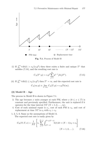
![178 7 Imperfect Preventive Maintenance
It is trivial that the expected cost rate is decreasing in x because the failure
rate h(t) is increasing.
We seek an optimum replacement number N∗
(1 ≤ N∗
≤ ∞) that
minimizes CB(N; T, x) for specified T 0 and x. From the inequality
CB(N + 1; T, x) ≥ CB(N; T, x), we have
L(N; T, x) ≥
(c3 − c2)
c1
(N = 1, 2, . . . ), (7.17)
where
L(N; T, x) ≡ N
T +N(T −x)
N(T −x)
h(t) dt −
N−1
j=0
T +j(T −x)
j(T −x)
h(t) dt
=
N−1
j=0
T
0
{h[t + N(T − x)] − h[t + j(T − x)]} dt (N = 1, 2, . . . ).
In addition, we have
L(N + 1; T, x) − L(N; T, x)
= (N + 1)
T
0
{h[t + (N +1)(T −x)] − h[t + N(T −x)]} dt 0.
Therefore, we have the following optimum policy.
(i) If L(∞; T, x) ≡ limN→∞ L(N; T, x) (c3 − c2)/c1 then there exists a
finite and unique minimum N∗
that satisfies (7.17).
(ii) If L(∞; T, x) ≤ (c3 − c2)/c1 then N∗
= ∞, and the expected cost rate is
CB(∞; T, x) ≡ lim
N→∞
CB(N; T, x) = c1h(∞) +
c2
T
.
We clearly have N∗
∞ if h(t) → ∞ as t → ∞.
(3) Model C – Rate
It is assumed that:
3. The age after PM reduces to at (0 a ≤ 1) when it was t before PM; i.e.,
the age becomes t(1 − a) units of time younger at each PM. Furthermore,
the unit is replaced if it operates for NT.
1, 2, 4, 5, 6. Same as the assumptions of Model B.
The expected cost rate is
CC(N; T, a) =
1
NT
⎡
⎣c1
N−1
j=0
(Aj +1)T
Aj T
h(t) dt + (N − 1)c2 + c3
⎤
⎦
(N = 1, 2, . . . ), (7.18)](https://image.slidesharecdn.com/maintenancetheoryofreliabilityspringerseriesinreliability-240303085250-86c4adaf/85/Maintenance_Theory_of_Reliability_Springer_Series_in_Reliability-pdf-186-320.jpg)

 at
each PM when it was x + T immediately before PM. If the operation of the
unit enters into the steady-state then we have the equation
1 −
c2
c0
(x + T) = x, i.e., x =
c0
c2
− 1
T. (7.22)
Thus, the expected cost rate is
CD(T; c0) =
1
T
#
c1
T
0
h(t + x) dt + c2
$
=
1
T
#
c1
(c0/c2)T
[(c0/c2)−1]T
h(t) dt + c2
$
. (7.23)
Differentiating CD(T; c0) with respect to T and setting it equal to zero,
(c0/c2)T
[(c0/c2)−1]T
t dh(t) =
c2
c1
. (7.24)
Next, suppose that the failure rate after PM reduces to [1−(c2/c0)]h(x+T)
at each PM where it was h(x + T) before PM. In the steady-state, we have
1 −
c2
c0
h(x + T) = h(x) (7.25)
and the expected cost rate is
CD(T; c0) =
1
T
#
c1
T
0
h(t + x) dt + c2
$
. (7.26)
Thus, the age after PM is computed from (7.25), and hence, an optimum PM
time T∗
is computed by substituting x into (7.26) and changing T to minimize
it.
We have considered four imperfect PM models and have obtained the
expected cost rates. It is noted that all models are identical and agree with
the standard model in Section 4.2 when p = 0 in Model A, N = 1 in Models B
and C, and c0 = c2 in Model D.](https://image.slidesharecdn.com/maintenancetheoryofreliabilityspringerseriesinreliability-240303085250-86c4adaf/85/Maintenance_Theory_of_Reliability_Springer_Series_in_Reliability-pdf-188-320.jpg)
![7.2 Preventive Maintenance with Minimal Repair 181
Example 7.2. We finally consider an example when the failure time has a
Weibull distribution and show how to determine optimum PM times. When
F(t) = 1 − exp(−λtm
) (λ 0, m 1), we have the following results for each
model.
(1) Model A
The expected cost rate is, from (7.13),
CA(T; p) =
1
T
[c1qλTm
g(m) + c2] ,
where g(m) ≡ q
∞
j=1 pj−1
jm
which represents the mth moment of the geo-
metric distribution with parameter p. The optimum PM time is, from (7.14),
T∗
=
c2
c1qλ(m − 1)g(m)
1/m
.
(2) Model B
The expected cost rate is, from (7.16),
CB(N; T, x)
=
1
NT
⎡
⎣c1λ
N−1
j=0
{[T + j(T − x)]m
− [j(T − x)]m
} + (N − 1)c2 + c3
⎤
⎦
and from (7.17),
N−1
j=0
{[T + N(T − x)]m
− [T + j(T − x)]m
− [N(T − x)]m
+ [j(T − x)]m
}
≥
c3 − c2
λc1
whose left-hand side is strictly increasing in N to ∞ for 0 ≤ x T. Thus,
there exists a finite and unique minimum N∗
(1 ≤ N∗
∞).
(3) Model C
The expected cost rate is, from (7.18),
CC(N; T, a) =
1
NT
⎡
⎣c1λTm
N−1
j=0
[(Aj + 1)m
− (Aj)m
] + (N − 1)c2 + c3
⎤
⎦](https://image.slidesharecdn.com/maintenancetheoryofreliabilityspringerseriesinreliability-240303085250-86c4adaf/85/Maintenance_Theory_of_Reliability_Springer_Series_in_Reliability-pdf-189-320.jpg)
![182 7 Imperfect Preventive Maintenance
and from (7.19),
Tm
N−1
j=0
[(AN + 1)m
− (Aj + 1)m
− (AN )m
+ (Aj)m
] ≥
c3 − c2
λc1
whose left-hand side is strictly increasing in N to ∞ because m 1. Thus,
there exists a finite and unique minimum N∗
(1 ≤ N∗
∞). Furthermore,
the left-hand side of the above equation is increasing in T for a fixed N and
m, and hence, the optimum N∗
is a decreasing function of T.
(4) Model D
The expected cost rate is, from (7.23),
CD(T; c0) =
1
T
c1λTm
c0
c2
m
−
c0
c2
− 1
m
+ c2
and the optimum PM time is, from (7.24),
T∗
=
c2
c1λ(m − 1) {(c0/c2)m − [(c0/c2) − 1]
m
}
1/m
.
Similarly, the expected cost rate in (7.26) is
CD(T; c0) =
1
T
{c1λTm
[Dm
− (D − 1)m
] + c2}
and hence, the optimum PM time is
T∗
=
c2
c1λ(m − 1)[Dm − (D − 1)m]
1/m
,
where
D ≡
1
1 − [1 − (c2/c0)]
1/(m−1)
.
7.3 Inspection with Preventive Maintenance
In this section, we check a unit periodically to see whether it is good, and
at the same time, provide preventive maintenance. For example, we test a
unit, and if needed, we make the overhaul and the repair or replacement of
bad parts. This policy could actually be applied to the models of production
machines, standby units, and preventive medical checks for diseases [23]. The
standard inspection policy is explained in detail in Chapter 8.](https://image.slidesharecdn.com/maintenancetheoryofreliabilityspringerseriesinreliability-240303085250-86c4adaf/85/Maintenance_Theory_of_Reliability_Springer_Series_in_Reliability-pdf-190-320.jpg)
![7.3 Inspection with Preventive Maintenance 183
We consider a modified inspection model in which the unit after inspection
has the same age as before with probability p and becomes as good as new
with probability q. Then, we obtain the following reliability quantities: (1)
the mean time to failure and (2) the expected number of inspections until
failure detection. When the failure rate is increasing, we investigate some
properties of these quantities. Furthermore, we derive the total expected cost
and the expected cost rate until failure detection. Optimum inspection times
that minimize the expected costs are given numerically where the failure time
has a Weibull distribution. Moreover, we propose two extended cases where
the age becomes younger at each inspection; i.e., the age becomes x units
of time younger at each inspection and the age after inspection reduces to at
when it was t before inspection. Finally, we consider two types of human error
at inspection and obtain the total expected cost.
7.3.1 Imperfect Inspection
Consider the periodic inspection policy with PM for a one-unit system that
should operate for an infinite time span.
1. The operating unit is inspected and maintained preventively at times kT
(k = 1, 2, . . . ) (0 T ∞).
2. The failed unit is detected only through inspection.
3. The unit after inspection has the same failure rate as it had before in-
spection with probability p (0 ≤ p ≤ 1) and becomes as good as new with
probability q ≡ 1 − p.
4. Cost of each inspection is c1 and cost of time elapsed between a failure
and its detection per unit of time is c2.
5. Inspection and PM times are negligible.
Let l(T; p) be the mean time to failure of a unit. Then, we can form the
renewal-type equation:
l(T; p) =
∞
j=1
pj−1
jT
(j−1)T
t dF(t) + pj−1
qF(jT)[jT + l(T; p)]
. (7.27)
The first term in the bracket on the right-hand side is the mean time until it
fails between (j−1)th and jth inspections, and the second term is the mean
time until it becomes new at the jth inspection, and after that, it fails. By
solving (7.27) and arranging it,
l(T; p) =
∞
j=0 pj
(j+1)T
jT
F(t) dt
∞
j=0 pj{F(jT) − F[(j + 1)T]}
. (7.28)
In particular, when p = 0, i.e., the unit always becomes as good as new
at each inspection,](https://image.slidesharecdn.com/maintenancetheoryofreliabilityspringerseriesinreliability-240303085250-86c4adaf/85/Maintenance_Theory_of_Reliability_Springer_Series_in_Reliability-pdf-191-320.jpg)
![184 7 Imperfect Preventive Maintenance
l(T; 0) =
1
F(T)
T
0
F(t) dt (7.29)
which agrees with (1.6) in Chapter 1. When p = 1, i.e., the unit after inspec-
tion has the same failure rate as before inspection, l(T; 1) = µ which is the
mean failure time of the unit.
Next, let M(T; p) be the expected number of inspections until failure de-
tection. Then, by a similar method to that of obtaining (7.27),
M(T; p) =
∞
j=1
pj−1
j{F[(j−1)T]−F(jT)}+ pj−1
qF(jT)[j+M(T; p)]
'
;
i.e.,
M(T; p) =
∞
j=0 pj
F(jT)
∞
j=0 pj
/
F(jT) − F[(j + 1)T]
0. (7.30)
In particular,
M(T; 0) =
1
F(T)
, M(T; 1) =
∞
j=0
F(jT). (7.31)
It is easy to see that
TF[(j + 1)T] ≤
(j+1)T
jT
F(t) dt ≤ TF(jT)
because F(t) is a nonincreasing function of t. Thus, from (7.28) and (7.30),
T[M(T; p) − 1] ≤ l(T; p) ≤ TM(T; p). (7.32)
Furthermore, it has been proved in [16] that if the failure rate is increasing
then both l(T; p) and M(T; p) are decreasing functions of p for a fixed T. From
this result, we have the inequalities
µ ≤ l(T; p) ≤
1
F(T)
T
0
F(t) dt (7.33)
∞
j=0
F(jT) ≤ M(T; p) ≤
1
F(T)
, (7.34)
where all equalities hold when F is exponential.
The total expected cost until failure detection is (see Equation (8.1) in
Chapter 8),](https://image.slidesharecdn.com/maintenancetheoryofreliabilityspringerseriesinreliability-240303085250-86c4adaf/85/Maintenance_Theory_of_Reliability_Springer_Series_in_Reliability-pdf-192-320.jpg)
![7.3 Inspection with Preventive Maintenance 185
Table 7.2. Optimum inspection time T ∗
for p and m when c1 = 10 and c2 = 1
m
p
1.0 1.5 2.0 2.5 3.0
0.00 97 171 236 289 330
0.01 97 170 234 286 328
0.05 97 168 228 275 314
0.10 97 164 219 262 295
0.20 97 158 204 237 260
0.30 97 151 189 214 231
0.40 97 144 175 195 207
C(T; p) =
∞
j=1
pj−1
jT
(j−1)T
[c1j + c2(jT − t)] dF(t)
+ pj−1
qF(jT)[c1j + C(T; p)]
.
Solving the above renewal equation with respect to C(T; p), we have
C(T; p) =
(c1 + c2T)
∞
j=0 pj
F(jT) − c2
∞
j=0 pj
(j+1)T
jT
F(t) dt
∞
j=0 pj{F(jT) − F[(j+1)T]}
= (c1 + c2T)M(T; p) − c2l(T; p). (7.35)
It is easy to see that limT →0 C(T; p) = limT →∞ C(T; p) = ∞. Thus, there
exists a finite and positive T∗
that minimizes the expected cost C(T; p). Also,
from the relation of (7.32), we have
c1l(T; p)
T
≤ C(T; p) ≤ c1M(T; p) + c2T. (7.36)
Example 7.3. We give a numerical example when the failure time has a
Weibull distribution with shape parameter m (m ≥ 1). Suppose that F(t) =
exp[−(λt)m
], 1/λ = 500, c1 = 10, and c2 = 1. Table 7.2 presents the optimum
inspection time T∗
that minimizes the expected cost C(T; p) for several values
of p and m. It is noted that optimum times T∗
are independent of p for the
particular case of m = 1. Except for m = 1, they are small when p is large.
The reason is that when the failure rate increases with age, it is better to
inspect early for large p.
7.3.2 Other Inspection Models
Consider two inspection models with PM where the age becomes younger at
each inspection. It is assumed that the age becomes x (0 ≤ x ≤ T) units of](https://image.slidesharecdn.com/maintenancetheoryofreliabilityspringerseriesinreliability-240303085250-86c4adaf/85/Maintenance_Theory_of_Reliability_Springer_Series_in_Reliability-pdf-193-320.jpg)
![186 7 Imperfect Preventive Maintenance
time younger at each inspection. Then, the probability that the unit does not
fail until time t is
S(t; T, x) = λ[k(T −x); t−kT]
k−1
*
j=0
λ[j(T −x); T] for kT ≤t(k+1)T,
(7.37)
where λ(t; x) ≡ [F(t + x) − F(t)]/F(t) is the probability that the unit with
age t fails during (t, t + x]. Thus, the mean time to failure is
l(T; x) =
∞
k=0
(k+1)T
kT
S(t; T, x) dt
=
∞
k=0
⎧
⎨
⎩
k−1
*
j=0
λ[j(T − x); T]
⎫
⎬
⎭
k(T −x)+T
k(T −x)
F(t) dt
F[k(T − x)]
, (7.38)
where
1−1
0 ≡ 1, and the expected number of inspections until failure detection
is
M(T; x) =
∞
k=0
kλ[k(T − x); T]
k−1
*
j=0
λ[j(T − x); T]
=
∞
k=0
k
*
j=0
λ[j(T − x); T]. (7.39)
Next, it is assumed that the age after inspection reduces to at (0 ≤ a ≤ 1)
where it was t before inspection. Then, in similar ways to those of obtaining
(7.38) and (7.39),
l(T; a) =
∞
k=0
⎧
⎨
⎩
k−1
*
j=0
λ[AjT; T]
⎫
⎬
⎭
(Ak+1)T
AkT
F(t) dt
F(AkT)
(7.40)
M(T; a) =
∞
k=0
k
*
j=0
λ[AjT; T], (7.41)
where Aj ≡ a + a2
+ · · · + aj
(j = 1, 2, . . . ) and A0 ≡ 0.
Note that the mean times l(T; ·) and the expected numbers M(T; ·) of three
models are equal in both cases of p = a = 0 and x = T (i.e., the unit becomes
as good as new by perfect inspection), and p = a = 1 and x = 0 (i.e., the unit
has the same age by imperfect inspection). Furthermore, substituting (7.38),
(7.39) and (7.40), (7.41) into (7.35), respectively, we obtain two expected costs
until failure detection.](https://image.slidesharecdn.com/maintenancetheoryofreliabilityspringerseriesinreliability-240303085250-86c4adaf/85/Maintenance_Theory_of_Reliability_Springer_Series_in_Reliability-pdf-194-320.jpg)
![7.3 Inspection with Preventive Maintenance 187
7.3.3 Imperfect Inspection with Human Error
It is well known that a high percentage of failures in most systems is directly
due to human error [48]. There are the following types of human error when
we inspect a standby unit at periodic times kT (k = 1, 2, . . . ) [2,49–51]:
1. Type A human error: The unit in a good state, i.e., in a normal condition,
is judged to be bad and is repaired.
2. Type B human error: The unit in a bad state, i.e., in a failed state, is
judged to be good.
It is assumed that the probabilities of type A error and type B error are
α and β, respectively, where 0 ≤ α + β 1. Then, the expected number of
inspections until a failed unit is detected is
∞
j=0
jβj−1
(1 − β) =
1
1 − β
.
Consider one cycle from time t = 0 to the time when a failed unit is
detected by perfect inspection or a good unit is repaired by type A error,
whichever occurs first. Then, the total expected cost of one cycle is given by
C(T; α, β) =
∞
j=0
(1 − α)j
# (j+1)T
jT
c1
j +
1
1 − β
dF(t)
+ αc1(j + 1)F((j + 1)T) +
(j+1)T
jT
c2
jT +
T
1 − β
− t
dF(t)
$
= (c1 + c2T)
⎧
⎨
⎩
1
1 − β
∞
j=0
(1 − α)j
[F(jT) − F((j + 1)T)]
+
∞
j=0
(1 − α)j
F((j + 1)T)
⎫
⎬
⎭
− c2
∞
j=0
(1 − α)j
(j+1)T
jT
F(t) dt. (7.42)
When α = β = 0, i.e., the inspection is perfect, Equation (7.42) is equal to
that of a standard periodic inspection policy (see Section 8.1).
In particular, when F(t) = 1 − e−λt
, the expected cost is rewritten as
C(T; α, β) = (c1 + c2T)
(1 − e−λT
)/(1 − β) + e−λT
1 − (1 − α)e−λT
−
c2
λ
1 − e−λT
1 − (1 − α)e−λT
.
(7.43)
Differentiating C(T; α, β) with respect to T and setting it equal to zero,
eλT
− 1
λ
[1 − β(1 − α)e−λT
] − (1 − α − β)T =
c1
c2
(1 − α − β). (7.44)
Note that the left-hand side of (7.44) is strictly increasing from 0 to ∞. There-
fore, there exists a finite and unique T∗
that satisfies (7.44).](https://image.slidesharecdn.com/maintenancetheoryofreliabilityspringerseriesinreliability-240303085250-86c4adaf/85/Maintenance_Theory_of_Reliability_Springer_Series_in_Reliability-pdf-195-320.jpg)

![7.4 Computer System with Imperfect Maintenance 189
p2
∞
j=1
pj−1
1 F(jT), (7.46)
and the probability that the system is renewed by repair after maintenance
failure is
p3
∞
j=1
pj−1
1 F(jT), (7.47)
where (7.45) + (7.46) + (7.47) = 1.
Furthermore, the mean time of one cycle from time t = 0 to the time when
the system is renewed by either repair or perfect maintenance is
∞
j=1
pj−1
1
jT
(j−1)T
t dF(t) + (p2 + p3)
∞
j=1
jTpj−1
1 F(jT)
= (1 − p1)
∞
j=1
pj−1
1
jT
0
F(t) dt. (7.48)
Therefore, the mean time to failure is
l(T; p1, p2, p3) =
∞
j=1
pj−1
1
jT
(j−1)T
t dF(t)
+ pj−1
1 F(jT) [p2(jT + l(T; p1, p2, p3)) + p3jT]
;
i.e.,
l(T; p1, p2, p3) =
(1 − p1)
∞
j=1 pj−1
1
jT
0
F(t) dt
1 − p2
∞
j=1 pj−1
1 F(jT)
(7.49)
which agrees with (5) of [11] when p3 = 0, and (9) of [13].
The availability is, from (6.10) in Chapter 6,
A(T; p1, p2, p3) =
(1 − p1)
∞
j=1 pj−1
1
jT
0
F(t) dt
#
(1 − p1)
∞
j=1 pj−1
1
jT
0
F(t) dt + β2p3
∞
j=1 pj−1
1 F(jT)
+β1(1 − p1)
∞
j=1 pj−1
1 F(jT)
$
(7.50)
which agrees with (10) of [11] when p3 = 0.
First, we seek an optimum PM time T∗
1 that maximizes MTTF l(T; p1, p2, p3)
in (7.49). It is evident that](https://image.slidesharecdn.com/maintenancetheoryofreliabilityspringerseriesinreliability-240303085250-86c4adaf/85/Maintenance_Theory_of_Reliability_Springer_Series_in_Reliability-pdf-197-320.jpg)
![190 7 Imperfect Preventive Maintenance
l(0; p1, p2, p3) ≡ lim
T →0
l(T; p1, p2, p3) = 0
l(∞; p1, p2, p3) ≡ lim
T →∞
l(T; p1, p2, p3) = µ. (7.51)
Thus, there exists some positive T∗
1 (0 T∗
1 ≤ ∞) that maximizes l(T; p1, p2, p3).
Differentiating l(T; p1, p2, p3) with respect to T and setting it equal to zero,
we have
H(T; p1)
∞
j=1
pj−1
1
jT
0
F(t) dt +
∞
j=1
pj−1
1 F(jT) =
1
p2
, (7.52)
where
H(T; p1) ≡
∞
j=1 pj−1
1 jf(jT)
∞
j=1 pj−1
1 jF(jT)
.
It can be shown that the left-hand side of (7.52) is strictly increasing from
1/(1 − p1) to µH(∞; p1)/(1 − p1) when H(t; p1) is strictly increasing. Thus,
the optimum policy is:
(i) If H(T; p1) is strictly increasing and H(∞; p1) (1−p1)/(µp2) then there
exists a finite and unique T∗
1 that satisfies (7.52), and the resulting MTTF
is
l(T∗
1 ; p1, p2, p3) =
1 − p1
p2H(T∗
1 ; p1)
. (7.53)
(ii) If H(T; p1) is nonincreasing, or H(T; p1) is strictly increasing and H(∞; p1) ≤
(1 − p1)/(µp2), then T∗
1 = ∞; viz, no PM should be done, and the MTTF
is given in (7.51).
Next, we seek an optimum PM time T∗
2 that maximizes the availability
A(T; p1, p2, p3) in (7.50). Differentiating A(T; p1, p2, p3) with respect to T and
setting it equal to zero imply
H(T; p1)
∞
j=1
pj−1
1
jT
0
F(t) dt +
∞
j=1
pj−1
1 F(jT) =
β1
β1(1 − p1) − β2p3
. (7.54)
Note that β1(1 − p1) β2p3 because β1 ≥ β2.
Thus, we have a similar optimum policy to the previous case. Also, it is of
interest that T∗
1 ≥ T∗
2 because β1/[β1(1 − p1) − β2p3] ≤ 1/p2.
Example 7.4. Consider a triple redundant system that consists of three units,
and fails when two or more units have failed. This system is a 2-out-of-3 system
and is applied to the design of a fail-safe system. The failure distribution of
the system is F(t) = 3e−2t
− 2e−3t
, and the mean time to failure is µ = 5/6.
In addition, we have](https://image.slidesharecdn.com/maintenancetheoryofreliabilityspringerseriesinreliability-240303085250-86c4adaf/85/Maintenance_Theory_of_Reliability_Springer_Series_in_Reliability-pdf-198-320.jpg)
![7.5 Sequential Imperfect Preventive Maintenance 191
H(t; p1) =
6
∞
j=1 pj−1
1 j(e−2jt
− e−3jt
)
∞
j=1 pj−1
1 j(3e−2jt − 2e−3jt)
H(0; p1) = 0, H(∞; p1) = 2
dH(t; p1)
6 dt
=
1
D
⎡
⎣6
∞
j=1
pj−1
1 j2
(e−2jt
− e−3jt
)
∞
j=1
pj−1
1 j(e−2jt
− e−3jt
)
−
∞
j=1
pj−1
1 j2
(2e−2jt
− 3e−3jt
)
∞
j=1
pj−1
1 j(3e−2jt
− 2e−3jt
)
⎤
⎦
=
1
D
⎡
⎣
∞
j=1
∞
i=1
pi+j−2
1 (i2
j)(3e−it
− 2e−jt
)e−2(i+j)t
⎤
⎦ 0,
where
D ≡
⎡
⎣
∞
j=1
pj−1
1 j(3e−2jt
− 2e−3jt
)
⎤
⎦
2
.
Thus, H(t; p1) is strictly increasing from 0 to 2.
Therefore, if 1 − p1 (5/2)(β2/β1)p3 then there exists a finite and unique
T∗
2 that satisfies
H(T; p1)
6
⎧
⎨
⎩
∞
j=1
pj−1
1 [9(1 − e−2jT
) − 4(1 − e−3jT
)]
⎫
⎬
⎭
+
∞
j=1
pj−1
1 (3e−2jT
− 2e−3jT
) =
β1
β1(1 − p1) − β2p3
and otherwise, T∗
2 = ∞.
Table 7.3 shows the optimum PM time T∗
2 (×102
) for p1 = 10−3
, 10−2
,
10−1
, p3 = 10−4
, 10−3
, 10−2
, 10−1
, and β2/β1 = 0.1, 1.0. For example, when
p1 = 0.1, p3 = 0.01, and β2/β1 = 0.1, T∗
2 = 1.72 × 10⁻²
. If the MTTF of
each unit is 104
hours then T∗
2 = 172 hours. These results indicate that the
system should be maintained about once a week. Furthermore, it is of great
interest that the optimum T∗
2 depends considerably on the product of β2/β1
and p3, but depends little on p1. When (β2/β1)p3 = 10−4
, 10−3
, 10−2
, 10−1
,
the approximate optimum times T∗
2 are 0.005, 0.018, 0.06, 0.28, respectively.
7.5 Sequential Imperfect Preventive Maintenance
We consider the following two PM policies, by introducing improvement fac-
tors [15,52] in failure rate and age for a sequential PM policy [53,54]: the PM](https://image.slidesharecdn.com/maintenancetheoryofreliabilityspringerseriesinreliability-240303085250-86c4adaf/85/Maintenance_Theory_of_Reliability_Springer_Series_in_Reliability-pdf-199-320.jpg)
![192 7 Imperfect Preventive Maintenance
Table 7.3. Optimum PM time T ∗
2 (×102
) to maximize availability A(T ; p1, p2, p3)
for p1, p2 and β2/β1
β2/β1 = 0.1 β2/β1 = 1.0
p3 p1
10−3
10−2
10−1
10−3
10−2
10−1
10−4
0.183 0.181 0.166 0.582 0.578 0.529
10−3
0.582 0.578 0.529 1.88 1.87 1.72
10−2
1.88 1.87 1.72 6.42 6.37 5.98
10−1
6.42 6.37 5.98 28.1 28.1 27.6
is done at fixed intervals Tk (k = 1, 2, . . . , N − 1) and is replaced at the Nth
PM; if the system fails between PMs, it undergoes only minimal repair. The
PM is imperfect as follows.
(1) The age after the kth PM reduces to akt when it was t before PM.
(2) The failure rate after the kth PM becomes bkh(t) when it was h(t) in the
period of the kth PM.
The imperfect PM model that combines two policies was considered in [55].
The expected cost rates of two models are obtained and optimum sequences
{T∗
k } are derived. When the failure time has a Weibull distribution, optimum
policies are computed explicitly.
(1) Model A – Age
Consider the sequential PM policy for a one-unit system for an infinite time
span. It is assumed that (see Figure 7.2):
1. The PM is done at fixed intervals Tk (k = 1, 2, . . . , N − 1) and is replaced
at the Nth PM; i.e., the unit is maintained preventively at successive
times T1 T1 + T2 · · · T1 + T2 + · · · + TN−1 and is replaced at time
T1 + T2 + · · · + TN , where T0 ≡ 0.
2. The unit undergoes only minimal repair at failures between replacements
and becomes as good as new at replacement.
3. The age after the kth PM reduces to akt when it was t before PM; i.e.,
the unit with age t becomes t(1 − ak) units of time younger at the kth
PM, where 0 = a0 a1 ≤ a2 ≤ · · · ≤ aN 1.
4. Cost of each minimal repair is c1, cost of each PM is c2, and cost of
replacement at the Nth PM is c3.
5. The times for PM, repair, and replacement are negligible.
The unit is aged from ak−1(Tk−1 + ak−2Tk−2 + · · · + ak−2ak−3 . . . a2a1T1)
after the (k−1)th PM to Tk+ak−1(Tk−1+ak−2Tk−2+· · ·+ak−2ak−3 . . . a2a1T1)
before the kth PM, i.e., from ak−1Yk−1 to Yk, where Yk ≡ Tk +ak−1Tk +· · ·+
ak−1ak−2 + · · · + a2a1T1 (k = 1, 2, . . . ), which is the age immediately before
the kth PM. Thus, the expected cost rate is](https://image.slidesharecdn.com/maintenancetheoryofreliabilityspringerseriesinreliability-240303085250-86c4adaf/85/Maintenance_Theory_of_Reliability_Springer_Series_in_Reliability-pdf-200-320.jpg)


![7.5 Sequential Imperfect Preventive Maintenance 195
CA(N) ≡
(N −1)c2 + c3
N−1
k=0 dk
(N = 1, 2, . . . ) (7.64)
which is the same problem as minimizing h(YN ), i.e., CA(Y1, Y2, . . . , YN ).
From the inequality CA(N + 1) ≥ CA(N), we have
LA(N) ≥
c3
c2
(N = 1, 2, . . . ), (7.65)
where
LA(N) ≡
N−1
k=0
dk
dN
− (N − 1) (N = 1, 2, . . . ). (7.66)
If dk is decreasing in k then LA(N) is increasing in N. Thus, there exists a
finite and unique minimum N∗
that satisfies (7.65) if LA(∞) c3/c2.
We show that dk is decreasing in k from the assumption that ak ak+1.
Let g(x) ≡ (1−x)m
/(1−xm
) (0 x 1) for m 1. Then, g(x) is decreasing
from 1 to 0, and hence,
(1 − ak)m
1 − am
k
(1 − ak+1)m
1 − am
k+1
which follows that dk dk+1. Furthermore, if ak → 1 as k → ∞ then
lim
k→∞
dk = lim
x→1
[g(x)]1/(m−1)
= 0;
i.e., LA(N) → ∞ as N → ∞, and a finite N∗
exists uniquely.
Therefore, if ak → 1 as k → ∞ then an N∗
is a finite and unique minimum
that satisfies (7.65), and the optimum intervals are T∗
k = Yk − ak−1Yk−1
(k = 1, 2, . . . , N∗
), where Yk and YN are given in (7.62) and (7.63).
For Model B, by solving Bkh(Tk) = D, we have
Tk =
D
mBk
1/(m−1)
(k = 1, 2, . . . , N). (7.67)
Substituting Tk into (7.61) and arranging it,
D =
#
(N − 1)c2 + c3
c1
(
1 − 1
m
) N
k=1 [(1/mBk)]
1/(m−1)
$(m−1)/m
(7.68)
which is a function of N. Let us denote D by D(N). Then, from the inequality
D(N + 1) ≥ D(N), an N∗
to minimize D is given by a unique minimum that
satisfies
LB(N) ≥
c3
c2
(N = 1, 2, . . . ), (7.69)](https://image.slidesharecdn.com/maintenancetheoryofreliabilityspringerseriesinreliability-240303085250-86c4adaf/85/Maintenance_Theory_of_Reliability_Springer_Series_in_Reliability-pdf-203-320.jpg)


![8
Inspection Policies
System reliability can be improved by providing some standby units. Espe-
cially, even a single standby unit plays an important role in the case where
failures of an operating unit are costly and/or dangerous. A typical example is
the case of standby electric generators in nuclear power plants, hospitals, and
other public facilities. It is, however, extremely serious if a standby generator
fails at the very moment of electric power supply stoppage. Hence, frequent
inspections are necessary to avoid such unfavorable situations.
Similar examples can be found in army defense systems, in which all
weapons are on standby, and hence, must be checked at suitable times. For
example, missiles are stored for a great part of their lifetimes after delivery.
However, their reliabilities are known to decrease with time because some
parts deteriorate with time. Thus, it would be important to test the functions
of missiles as to whether they can operate normally. We need to check them
periodically to monitor their reliabilities and to repair them if necessary.
Earlier work has been done on the problem of checking a single unit. The
optimum schedules of inspections that minimize two expected costs until fail-
ure detection and per unit of time were summarized in [1]. The modified
models where checking times are nonnegligible, a unit is inoperative during
checking times, and checking hastens failures and failure symptoms, were con-
sidered in [2–5]. Furthermore, the availability of a periodic inspection model [6]
and the mean duration of hidden faults [7,8] were derived. The downtime cost
of checking intervals for a continuous production process [9,10] and two types
of inspection [11,12] were proposed. The optimum inspection policies for more
complicated systems were discussed in [13–20]. A good survey of optimization
problems for inspection models was made in [21].
It was difficult to compute an optimum solution of the algorithm presented
by [1] before high-power computers were popular. Nearly optimum inspection
policies were considered in [22–28]. A continuous inspection intensity was in-
troduced and the approximate checking interval was derived in [29,30]. Using
these approximate methods, some modified inspection models were discussed
and compared with other methods [31–37].
201](https://image.slidesharecdn.com/maintenancetheoryofreliabilityspringerseriesinreliability-240303085250-86c4adaf/85/Maintenance_Theory_of_Reliability_Springer_Series_in_Reliability-pdf-208-320.jpg)
![202 8 Inspection Policies
All failures cannot be detected upon inspection. The imperfect inspection
models were treated in [38–41], and the parameter of an exponential failure
distribution was estimated in [42]. Furthermore, optimum inspection models
for a unit with hidden failure [43] were discussed in [44]. In such models, even
if a unit fails, it continues to operate in hidden failure, and then, it fails. Such
a type of failure is called unrevealed fault [45], pending failure [25], or fault
latency [47].
Most faults occur intermittently in digital systems. The optimum periodic
tests for intermittent faults were discussed in [48–50]. A simple algorithm to
compute an optimum time was developed in [51], and random test for fault
detection in combinational circuits was introduced in [52].
It is especially important to check and maintain standby and protective
units. The optimum inspection models for standby units [53–57] and protec-
tive devices [59–61] were presented. Also, the following inspection maintenance
to actual systems was done: building, industrial plant, and underwater struc-
ture [62–64]; combustion turbine units and standby equipment in dormant
systems and nuclear generating stations [65–67]; productive equipment [68];
fail-safe structure [69]; manufacturing station [70]; automatic trips and warn-
ing instruments [71]; bearing [72]; and safety-critical systems [73]. Moreover,
the delay time models were reviewed in [74,75], where a defect arises and be-
comes a failure after its delay time, and were applied to plant maintenance [76].
This chapter reviews the results of [1] and mainly summarizes our own
results of inspection models. In Section 8.1, we briefly mention the results
of [1], and consider the inspection model with finite number of checks [77].
In Section 8.2, we summarize four approximate inspection policies [31–35,78].
In Section 8.3, we derive two optimum inspection policies for a standby unit
as an example of an electric generator [53]. In Section 8.4, we consider the
inspection policy for a storage system required to achieve a high reliability,
and derive an optimum checking number until overhaul that minimizes the
expected cost rate [80–83]. In Section 8.5, we discuss optimum testing times
for intermittent faults [49, 50]. Finally, in Section 8.6, we rewrite the results
of a standard model for inspection policies for units that have to be operating
for a finite interval [84,85]. It is shown that the proposed partition method is
a useful technique for analyzing maintenance policies for a finite interval. The
inspection with preventive maintenance and random inspection is covered in
Sections 7.3 and 9.3, respectively.
8.1 Standard Inspection Policy
A unit should operate for an infinite time span and is checked at successive
times Tk (k = 1, 2, . . . ), where T0 ≡ 0 (see Figure 8.1). Any failure is detected
at the next checking time and is replaced immediately. A unit has a failure
distribution F(t) with finite mean µ whose failure rate h(t) is not unchanged
by any check. It is assumed that all times needed for checks and replacement](https://image.slidesharecdn.com/maintenancetheoryofreliabilityspringerseriesinreliability-240303085250-86c4adaf/85/Maintenance_Theory_of_Reliability_Springer_Series_in_Reliability-pdf-209-320.jpg)
![8.1 Standard Inspection Policy 203
Failure Detection of failure
Downtime from failure to detection
0
T1 T2 T3 Tk−1 Tk
Fig. 8.1. Process of sequential inspection with checking time Tk
are negligible. Let c1 be the cost of one check and c2 be the loss cost per unit
of time for the time elapsed between a failure and its detection at the next
checking time, and c3 be the replacement cost of a failed unit. Then, the total
expected cost until replacement is
C1(T1, T2, . . . ) ≡
∞
k=0
Tk+1
Tk
[c1(k + 1) + c2(Tk+1 − t)] dF(t) + c3
=
∞
k=0
[c1 + c2(Tk+1 − Tk)]F(Tk) − c2µ + c3, (8.1)
where throughout this chapter, we use the notation Φ ≡ 1 − Φ.
Differentiating the expected cost C1(T1, T2, . . . ) with Tk and putting it
equal to zero,
Tk+1 − Tk =
F(Tk) − F(Tk−1)
f(Tk)
−
c1
c2
(k = 1, 2, . . . ), (8.2)
where f is a density function of F. The optimum checking intervals are de-
creasing when f is PF2 (Pólya frequency function of order 2), and Algorithm
1 for computing the optimum inspection schedule is given in [1].
Algorithm 1
1. Choose T1 to satisfy c1 = c2
T1
0
F(t)dt.
2. Compute T2, T3, . . . recursively from (8.2).
3. If any δk δk−1, reduce T1 and repeat, where δk ≡ Tk+1 − Tk. If any
δk 0, increase T1 and repeat.
4. Continue until T1 T2 . . . are determined to the degree of accuracy
required.
Clearly, because the mean time to replacement time is
∞
k=0(Tk+1 −
Tk)F(Tk), the expected cost rate is, from (3.3) in Chapter 3,
C2(T1, T2, . . . ) ≡
c1
∞
k=0 F(Tk) − c2µ + c3
∞
k=0(Tk+1 − Tk)F(Tk)
+ c2. (8.3)
In particular, when a unit is checked at periodic times and the failure time
is exponential, i.e., Tk = kT (k = 0, 1, 2, . . . ) and F(t) = 1 − e−λt
, the total
expected cost is](https://image.slidesharecdn.com/maintenancetheoryofreliabilityspringerseriesinreliability-240303085250-86c4adaf/85/Maintenance_Theory_of_Reliability_Springer_Series_in_Reliability-pdf-210-320.jpg)
![204 8 Inspection Policies
C1(T) =
c1 + c2T
1 − e−λT
−
c2
λ
+ c3. (8.4)
The optimum checking time T∗
to minimize (8.4) is given by a unique solution
that satisfies
eλT
− (1 + λT) =
λc1
c2
. (8.5)
Similarly, the expected cost rate is
C2(T) =
c1 − (c2/λ − c3)(1 − e−λT
)
T
+ c2. (8.6)
When c2/λ c3, the optimum T∗
is given by solving
1 − (1 + λT)e−λT
=
c1
c2/λ − c3
. (8.7)
The following total expected cost for a continuous production system was
proposed in [9].
C1(T1, T2, . . . ) ≡
∞
k=0
Tk+1
Tk
[c1(k + 1) + c2(Tk+1 − Tk)] dF(t) + c3
= c1
∞
k=0
F(Tk) + c2
∞
k=0
(Tk+1 − Tk)[F(Tk) − F(Tk+1)] + c3.
(8.8)
In this case, Equation (8.2) can rewritten as
Tk+1 − 2Tk + Tk−1 =
F(Tk+1) − 2F(Tk) + F(Tk−1)
f(Tk)
−
c1
c2
(k = 1, 2, . . . ). (8.9)
In general, it would be important to consider the availability more than the
expected cost in some production systems [86,87]. Let β1 be the time of one
check and β3 be the replacement time of a failed unit. Then, the availability
is, from (3) of Section 2.1.1,
A(T1, T2, . . . ) ≡
∞
0
F(t) dt
∞
k=0[β1 + Tk+1 − Tk]F(Tk) + β3
.
Thus, the policy maximizing A(T1, T2, . . . ) is the same one as minimizing
C1(T1, T2, . . . ) in (8.1) by replacing ci = βi (i = 1, 3) and c2 = 1.
Next, we consider the inspection model with a finite number of checks,
because a system such as missiles involves some parts that have to be replaced
when the total operating times of checks have exceeded a prespecified time
of quality warranty. A unit is checked at times Tk (k = 1, 2, . . . , N − 1) and](https://image.slidesharecdn.com/maintenancetheoryofreliabilityspringerseriesinreliability-240303085250-86c4adaf/85/Maintenance_Theory_of_Reliability_Springer_Series_in_Reliability-pdf-211-320.jpg)
![8.1 Standard Inspection Policy 205
is replaced at time TN (N = 1, 2, . . . ). The periodic inspection policy was
suggested in [86], where a system is maintained preventively at the Nth check
or is replaced at failure, whichever occurs first. We may consider replacement
as preventive maintenance or overhaul.
In the above finite inspection model, the expected cost when a failure is
detected and a unit is replaced at time Tk (k = 1, 2, . . . , N) is
N
k=1
Tk
Tk−1
[c1k + c2(Tk − t) + c3] dF(t)
and the expected cost when a unit is replaced without failure at time TN is
(c1N + c3)F(TN ).
Thus, the total expected cost until replacement is
N−1
k=0
[c1 + c2(Tk+1 − Tk)]F(Tk) − c2
TN
0
F(t) dt + c3.
Similarly, the mean time to replacement is
N
k=1
Tk
Tk−1
Tk dF(t) + TN F(TN ) =
N−1
k=0
(Tk+1 − Tk)F(Tk).
Therefore, the expected cost rate is
C2(T1, T2, . . . , TN ) =
c1
N−1
k=0 F(Tk) − c2
TN
0
F(t) dt + c3
N−1
k=0 (Tk+1 − Tk)F(Tk)
+ c2. (8.10)
In particular, when Tk = kT (k = 1, 2, . . . , N) and F(t) = 1 − e−λt
, the
expected cost rate is
C2(T) =
c1
T
−
1
λT
(1 − e−λT
)
c2 −
c3λ
1 − e−λNT
+ c2. (8.11)
Differentiating C2(T) with respect to T and putting it to 0, we have
c2
λ
−
c3
1−e−λNT
[1−(1+λT)e−λT
] −
c3λNTe−λNT
(1 − e−λT
)
(1−e−λNT )2
= c1. (8.12)
Denoting the left-hand side of (8.12) by QN (T), limT →0 QN (T) = −c3/N
and limT →∞ QN (T) = c2/λ − c3. First, we prove that QN (T) is an increasing
function of T for c2/λ c1 + c3. It is noted that the first term in QN (T)
is strictly increasing in T. Differentiating −Te−λNT
(1 − e−λT
)/(1 − e−λNT
)2
with respect to T,](https://image.slidesharecdn.com/maintenancetheoryofreliabilityspringerseriesinreliability-240303085250-86c4adaf/85/Maintenance_Theory_of_Reliability_Springer_Series_in_Reliability-pdf-212-320.jpg)
![206 8 Inspection Policies
A[λNT(1 − e−λT
)(1 + e−λNT
) − (1 − e−λNT
)(1 − e−λT
+ λTe−λT
)],
where A ≡ e−λNT
/(1 − e−λNT
)3
0 for T 0. Denoting the quantity in the
bracket of the above equation by LN (T),
L1(T) = (1 − e−λT
)(λT − 1 + e−λT
) 0
LN+1(T) − LN (T) = (1 − e−λT
)[λT(1 − Ne−λNT
+ Ne−λ(N+1)T
)
− (1 − e−λT
)e−λNT
]
(1 − e−λT
)2
[1 − (N + 1)e−λNT
+ Ne−λ(N+1)T
] 0.
Hence, LN (T) is strictly increasing in N. Thus, LN (T) is always positive
for any N, and the second term of QN (T) is an increasing function of T,
which completes the proof. Therefore, there exists a finite and unique T∗
N
(0 T∗
N ∞) that satisfies (8.12) for c2/λ c1 + c3, and it minimizes C2(T)
in (8.11).
Next, we investigate properties of T∗
N . We prove that QN (T) is also an
increasing function of N as follows. From (8.12),
QN+1(T) − QN (T) = c3(1 − e−λT
)[1 − EN (T)]
×
1 − (1 + λT)e−λT
EN (T)EN+1(T)
+ λT
N
EN (T)2
−
(N + 1)e−λT
EN+1(T)2
,
where EN (T) ≡ 1−e−λNT
. The first term in the bracket of the above equation
is positive. The second term can be rewritten as
N
EN (T)2
−
(N + 1)e−λT
EN+1(T)2
=
NEN+1(T)2
− (N + 1)e−λT
EN (T)2
EN (T)2EN+1(T)2
and the numerator of the right-hand side is
NEN+1(T)2
− (N + 1)e−λT
EN (T)2
= e−λT
[N(eλT
− 1)(1 − e−λ(2N+1)T
) − (1 − e−λNT
)2
] 0.
Hence, QN (T) is a strictly increasing function of N because QN+1(T) −
QN (T) 0. Thus, T∗
N decreases when N increases. When N = 1, we have
from (8.12),
1 − (1 + λT)e−λT
=
(c1 + c3)λ
c2
(8.13)
and when N = ∞,
1 − (1 + λT)e−λT
=
c1λ
c2 − c3λ
. (8.14)
Because [(c1 + c3)λ]/c2 c1λ/(c2 − c3λ), we easily find that T∗
∞ T∗
N ≤ T∗
1 ,
where T∗
1 and T∗
∞ are the respective solutions of (8.13) and (8.14).](https://image.slidesharecdn.com/maintenancetheoryofreliabilityspringerseriesinreliability-240303085250-86c4adaf/85/Maintenance_Theory_of_Reliability_Springer_Series_in_Reliability-pdf-213-320.jpg)
![8.2 Asymptotic Inspection Schedules 207
Table 8.1. Optimum checking time T ∗
N when c1 = 10, c2 = 1, and c3 = 100
λ = 1.0 × 10⁻³
λ = 1.1 × 10⁻³
λ = 1.2 × 10⁻³
N m
1.0 1.1 1.2 1.3 1.0 1.1 1.2 1.3 1.0 1.1 1.2 1.3
1 564 436 355 309 543 423 347 307 526 412 341 307
2 396 315 259 223 380 304 251 219 367 294 245 217
3 328 268 224 193 314 258 216 188 303 249 210 185
4 289 243 206 178 277 233 198 173 267 225 192 169
5 264 228 195 170 253 218 188 165 243 210 181 161
6 246 217 189 165 236 208 181 160 226 200 174 156
7 233 210 184 162 223 200 176 157 214 192 170 154
8 222 204 181 161 212 194 173 156 204 186 167 153
9 214 200 179 160 204 190 171 155 196 182 165 152
10 207 196 178 160 197 187 170 155 189 179 163 152
The condition of c2/λ c1 + c3 means that the total loss cost until the
whole life of a unit is higher than the sum of costs of checks and replacements.
This would be realistic in the actual field.
Example 8.1. We compute the optimum checking time T∗
N that minimizes
C2(T) in (8.11) when F(t) = 1 − exp(−λtm
) (m ≥ 1). When m = 1, it
corresponds to an exponential case. Table 8.1 shows the optimum time T∗
N
for λ = 1.0 × 10⁻³
, 1.1 × 10⁻³
, 1.2 × 10⁻³
/hour, m = 1.0, 1.1, 1.2, 1.3 and
N = 1, 2, . . . , 10 when c1 = 10, c2 = 1, and c3 = 100. This indicates that T∗
N
decreases when λ, m, and N increase, and that a unit should be checked once
every several weeks.
8.2 Asymptotic Inspection Schedules
The computing procedure for obtaining the optimum inspection schedule was
specified in [1]. Unfortunately, it is difficult to compute Algorithm 1 numeri-
cally, because the computations are repeated until the procedures are deter-
mined to the required degree by changing the first checking time. To avoid
this, a nearly optimum inspection policy that depends on a single parameter
p was suggested in [22]. This policy was used for Weibull and gamma distri-
bution cases [23,24]. Furthermore, the procedure of introducing a continuous
intensity n(t) of checks per unit of time was proposed in [29,30]. This section
summarizes four approximate calculations of optimum checking procedures.
(1) Periodic Inspection
When a unit is checked at periodic times kT (k = 1, 2, . . . ), the total expected
cost is, from (8.1),](https://image.slidesharecdn.com/maintenancetheoryofreliabilityspringerseriesinreliability-240303085250-86c4adaf/85/Maintenance_Theory_of_Reliability_Springer_Series_in_Reliability-pdf-214-320.jpg)
![208 8 Inspection Policies
C1(T) =
c1
T
[E{D} + µ] + c2E{D} + c3, (8.15)
where E{D} ≡
∞
k=0
T
0
[F(t + kT) − F(kT)] dt, which is the mean duration
of time elapsed between a failure and its detection.
Suppose that F(t) has the piecewise linear approximation:
F(t + kT) − F(kT) =
t
T
[F((k + 1)T) − F(kT)] (0 ≤ t ≤ T). (8.16)
Then, E{D} = T/2; i.e., the mean duration of undetected failure is half the
time between the checking times. The result is also given when the failure
times between successive checking times are independent and distributed uni-
formly. In this case, the optimum checking time is
T1 =
(2c1µ)/c2. This time
is also derived from (8.5) by putting eλT
≈ 1 + λT + (λT)2
/2 approximately
and λ = 1/µ.
(2) Munford and Shahani’s Method
The asymptotic method for computing the optimum schedule was proposed
in [22]. When a unit is operating at time Tk−1, the probability that it fails in
an interval (Tk−1, Tk] is constant for all k; i.e.,
F(Tk) − F(Tk−1)
F(Tk−1)
≡ p (k = 1, 2, . . . ). (8.17)
This represents that the probability that a unit with age Tk−1 fails in interval
(Tk−1, Tk] is given by a constant p. Noting that F(T1) = p, Equation (8.17)
can be solved for Tk, and we have
F(Tk) = qk
or Tk = F
−1
(qk
) (k = 1, 2, . . . ), (8.18)
where q ≡ 1 − p (0 p 1). Thus, from (8.1), the total expected cost is
C1(p) =
c1
p
+ c2
∞
k=1
Tkqk−1
p − c2µ + c3. (8.19)
We seek p that minimizes C1(p) in (8.19). It was assumed in [28] that p is not
constant and is an increasing function of the checking number.
(3) Keller’s Method
An inspection intensity n(t) is defined as follows [29]: n(t)dt denotes the prob-
ability that a unit is checked at interval (t, t + dt) (see Figure 8.2). From this
definition, when a unit is checked at times Tk, we have the relation
Tk
0
n(t) dt = k (k = 1, 2, . . . ). (8.20)](https://image.slidesharecdn.com/maintenancetheoryofreliabilityspringerseriesinreliability-240303085250-86c4adaf/85/Maintenance_Theory_of_Reliability_Springer_Series_in_Reliability-pdf-215-320.jpg)
![8.2 Asymptotic Inspection Schedules 209
any size is 1
t
n(t)
0 T1 T2 T3 T4 T5
Fig. 8.2. Inspection intensity n(t)
Furthermore, suppose that the mean time from the failure at time t to its
detection at time t + a is half of a checking interval, the same as obtained in
case (1). Then, we have
t+a
t
n(u) du =
1
2
which can be approximately written as
t+a
t
n(u) du ≈ an(t) =
1
2
and hence, a = 1/[2n(t)]. By the same arguments, we can easily see that
the next checking interval, when a unit was checked at time Tk, is 1/n(Tk)
approximately.
Therefore, the total expected cost in (8.1) is given by
C(n(t)) =
∞
0
c1
t
0
n(u) du +
c2
2n(t)
dF(t) + c3
=
∞
0
F(t)
c1n(t) +
c2h(t)
2n(t)
dt + c3, (8.21)
where h(t) ≡ f(t)/F(t) which is the failure rate. Differentiating C(n(t)) with
n(t) and putting it to zero,
n(t) =
%
c2h(t)
2c1
. (8.22)
Thus, from (8.20), the optimum checking time is given by the equation:](https://image.slidesharecdn.com/maintenancetheoryofreliabilityspringerseriesinreliability-240303085250-86c4adaf/85/Maintenance_Theory_of_Reliability_Springer_Series_in_Reliability-pdf-216-320.jpg)
![210 8 Inspection Policies
k =
Tk
0
2
c2
2c1
h(t) dt (k = 1, 2, . . . ). (8.23)
The inspection intensity n(t) was also obtained in [36] by solving the Eu-
ler equation in (8.21), and using n(t), the optimum policies for models with
imperfect inspection were derived in [88].
In particular, when F(t) = 1−e−λt
, the interval between checks is constant,
and is
2c1/(λc2) which agrees with the result of case (1). It is of great
interest that a function
2c1/(λc2) evolves into the same form as an optimum
order time of a classical inventory control model [89], by denoting c1 and c2
as the ordering cost per order and holding cost per unit of time, respectively,
and λ as the constant demand rate for an inventory unit.
(4) Nakagawa and Yasui’s Method
When Tn is sufficiently large, we may assume approximately [79]
Tn+1 − Tn + ε = Tn − Tn−1. (8.24)
It is easy to see that if f is PF2 then ε ≥ 0 because the optimum checking
intervals are decreasing [1]. Further substituting the relation (8.24) into (8.2),
c1
c2
− ε =
Tn
Tn−1
[f(t) − f(Tn)] dt
f(Tn)
≥ 0 (8.25)
because f(t) ≥ f(Tn) for t ≤ Tn and large Tn. Thus, we have 0 ≤ ε ≤ c1/c2.
From the above discussion, we can specify the computation for obtaining
the asymptotic inspection schedule.
Algorithm 2
1. Choose an appropriate ε from 0 ε c1/c2.
2. Determine a checking time Tn after sufficient time for required accuracy.
3. Compute Tn−1 to satisfy
Tn − Tn−1 − ε =
F(Tn) − F(Tn−1)
f(Tn)
−
c1
c2
.
4. Compute Tn−1 Tn−2 . . . recursively from (8.2).
5. Continue until Tk 0 or Tk+1 − Tk Tk.
Example 8.2. Suppose that the failure time has a Weibull distribution with
a shape parameter m; i.e., F(t) = 1 − exp[−(λt)m
].
(1) Periodic inspection. The optimum checking time is
λ
T1 =
2λc1
c2
Γ
!
1 +
1
m
1/2
.](https://image.slidesharecdn.com/maintenancetheoryofreliabilityspringerseriesinreliability-240303085250-86c4adaf/85/Maintenance_Theory_of_Reliability_Springer_Series_in_Reliability-pdf-217-320.jpg)
![8.2 Asymptotic Inspection Schedules 211
Table 8.2. Comparisons of Nakagawa, Barlow, Munford, and Keller policies when
F (t) = 1 − exp[−(λt)2
], 1/λ = 500, and c1/c2 = 10
Nakagawa Barlow Munford Keller
k Tn = 1500 p = 0.215
ε = 5 ε = 4.5
1 219.6 207.1 205.6 205.6 246.0 177.8
2 318.7 308.9 307.6 307.6 347.9 282.3
3 402.0 393.5 392.3 392.3 426.1 369.9
4 476.4 468.7 467.5 467.5 492.0 448.1
5 544.8 537.6 536.4 536.5 550.1 520.0
6 608.7 601.9 600.7 600.8 602.6 587.2
7 669.1 662.6 661.5 661.6 650.9 650.8
8 726.6 720.4 719.2 719.4 695.8 711.4
9 781.7 775.8 774.6 774.8 738.0 769.5
10 834.8 829.1 827.8 828.2 777.9 825.5
11 886.1 880.6 879.3 879.7 815.9 879.6
12 935.8 930.5 929.1 929.7 852.2 932.2
13 984.1 979.0 977.4 978.3 887.0 983.3
14 1031.1 1026.2 1024.5 1025.6 920.5 1033.1
(2) Munford and Shahani’s method. From (8.19), we obtain p that minimizes
g(p) =
λc1
pc2
+
log
1
q
1/m ∞
k=1
k1/m
qk−1
p
and the optimum checking intervals are
λTk =
k log
1
q
1/m
(k = 1, 2, . . . ).
(3) Keller’s method. From (8.23),
Tk =
(m + 1)k
2
c1
2mλmc2
2/(m+1)
(k = 1, 2, . . . ).
In particular, when m = 1, Tk = k
2c1/(λc2).
Table 8.2 shows the comparisons of the methods of Barlow et al., Munford
et al., Keller, and Nakagawa et al., when m = 2, 1/λ = 500, c1/c2 = 10.
Nakagawa and Yasui’s method gives a fairly good approximation of Barlow’s
one. In particular, when we choose ε = 4.5, the results are almost the same as
the sequence of optimum checking times. The computation of Keller’s method
is very easy, and this method would be very useful for obtaining checking times
in the actual field.](https://image.slidesharecdn.com/maintenancetheoryofreliabilityspringerseriesinreliability-240303085250-86c4adaf/85/Maintenance_Theory_of_Reliability_Springer_Series_in_Reliability-pdf-218-320.jpg)

![8.3 Inspection for a Standby Unit 213
In addition, let M0(t) and M1(t) be the expected numbers of repairs of a
failed generator and of checks of a standby generator during (0, t], respectively.
Then, the following renewal-type equations are given by
M0(t) =
t
0
F(u) dD(u) + H(t) ∗ M0(t) (8.27)
M1(t) = D(t) + H(t) ∗ M1(t). (8.28)
Thus, forming the Laplace–Stieltjes (LS) transforms of (8.26), (8.27), and
(8.28), respectively, we have
H∗
(s) = e−sT
[F(T) + F(T)G∗
(s)] (8.29)
M∗
0 (s) =
e−sT
F(T)
1 − H∗(s)
, M∗
1 (s) =
e−sT
1 − H∗(s)
, (8.30)
where throughout this section, we denote the LS transform of the function by
the corresponding asterisk; e.g., G∗
(s) ≡
∞
0
e−st
dG(t) for s 0.
Next, let P(t) denote the probability that a standby generator has failed
at time t; i.e., a standby generator, which is not good, will be detected at the
next check or a failed generator, which was detected at the prior check, is now
under repair. Then, the probability that a standby generator is good at time
t is given by
P(t) = F(t)D(t) + H(t) ∗ P(t).
Forming the LS transform of P(t), we have
1 − P∗
(s) =
T
0
se−st
F(t) dt
1 − H∗(s)
. (8.31)
We consider the total expected cost until the time of electric power supply
stoppage. Note that the inspection model of a standby generator may involve
at least the following three costs: the costs c0 and c1 incurred by each repair
and each check, respectively, and the cost c2 incurred by failure of a standby
generator when the electric power supply stops.
Suppose that the electric power supply stops at time t. Then, the total
expected cost during (0, t] is given by
C(t) = c0M0(t) + c1M1(t) + c2P(t).
Thus, dropping the condition that the electric power supply stops at time t
from assumption (6), we have the expected cost:
C1(T) ≡
∞
0
C(t)αe−αt
dt = c0M∗
0 (α) + c1M∗
1 (α) + c2P∗
(α)
which is a function of T. Using (8.30) and (8.31), C1(T) can be written as](https://image.slidesharecdn.com/maintenancetheoryofreliabilityspringerseriesinreliability-240303085250-86c4adaf/85/Maintenance_Theory_of_Reliability_Springer_Series_in_Reliability-pdf-220-320.jpg)
![214 8 Inspection Policies
C1(T) =
e−αT
[c0F(T) + c1] − c2
T
0
αe−αT
F(t) dt
1 − e−αT [F(T) + F(T)G∗(α)]
+ c2. (8.32)
It is evident that
C1(0) ≡ lim
T →0
C1(T) = ∞, C1(∞) ≡ lim
T →∞
C1(T) = c2F∗
(α)
which represents the expected cost for the case where no inspection is made.
We seek an optimum checking time T∗
1 that minimizes the expected cost
C1(T) given in (8.32). Differentiating log C1(T) with respect to T, we have,
for large T,
d[log C1(T)]
dT
≈ αe−αT
c2G∗
(α) − c0 − c1
c2F∗(α)
− G∗
(α)
.
Thus, if the quantity in the bracket on the right-hand side is positive; i.e.,
c2G∗
(α)[1 − F∗
(α)] c0 + c1, (8.33)
then there exists at least some finite T such that C1(∞) C1(T), and hence,
it is better to check a standby generator at finite time T.
In general, it is difficult to discuss analytically an optimum checking time
T∗
that minimizes C1(T). In particular, consider the case where F(t) = 1 −
e−λt
and G(t) ≡ 1 for t ≥ 0; i.e., the failure time is exponential and the repair
time is negligible. Then, the resulting cost is
C1(T) =
e−αT
[c0(1−e−λT
) + c1] + c2[1−e−αT
− α
α+λ (1−e−(α+λ)T
)]
1 − e−αT
. (8.34)
Differentiating C1(T) with respect to T and setting it equal to zero,
c0e−λT
1+
λ
α
(1 − e−αT
)
+ c2
1 − e−λT
−
λ
α+λ
(1 − e−(α+λ)T
)
= c0 + c1,
(8.35)
where the left-hand side is strictly increasing in the case of c2 [(α+λ)/α]c0,
and conversely, nonincreasing in the case of c2 ≤ [(α + λ)/α]c0. Further note
that the left-hand side is c0 as T → 0 and [α/(α + λ)]c2 as T → ∞.
Therefore, we have the following results from the above discussion.
(i) If c2 [(α + λ)/α](c1 + c0) then there exists a finite checking time T∗
1
that satisfies (8.35), and the resulting cost is
C1(T∗
) = c2 − c1 − c0 −
c2 − c0
α + λ
α
e−λT ∗
. (8.36)
(ii) If c2 ≤ [(α + λ)/α](c1 + c0) then T∗
1 = ∞; i.e., no inspection is made, and
C1(∞) = c2[λ/(α + λ)].](https://image.slidesharecdn.com/maintenancetheoryofreliabilityspringerseriesinreliability-240303085250-86c4adaf/85/Maintenance_Theory_of_Reliability_Springer_Series_in_Reliability-pdf-221-320.jpg)
 has been already derived
from (8.33).
It is also of interest to make the probability as small as possible by checks,
that a standby generator has failed at the time of electric power supply stop-
page. If the probability is prespecified, we can compute a checking time T1
such that P∗
(α) ≤ ε; i.e.,
T
0
e−αt
dF(t) − e−αT
F(T)G∗
(α)
1 − e−αT [F(T) + F(T)G∗(α)]
≤ ε. (8.37)
For instance, if the repair time is negligible, i.e., G∗
(α) = 1, then the left-hand
side of (8.37) is strictly increasing in T. Hence, there exists a unique checking
time T that satisfies T
0
F(t)αe−αt
dt
1 − e−αT
= ε (8.38)
for sufficiently small ε 0.
Until now, we have assumed that a standby generator becomes as good as
new upon inspection. Next, we make the same assumption as the previous ones
except that the failure rate of a standby generator remains undisturbed by
any inspection. This assumption would be more plausible than the previous
model in practice, however, the analysis becomes more difficult. Then, the
expected cost until the time of electric power supply stoppage is [53]
C2(T) =
c0
∞
k=1 e−αkT
[F((k − 1)T) − F(kT)]
+ c1
∞
k=1 e−αkT
F((k − 1)T) − c2[1 − F∗
(α)]
1 − G∗(α)
∞
k=1 e−αkT [F((k − 1)T) − F(kT)]
+ c2. (8.39)
It is evident that C2(0) = ∞ and C2(∞) = c2F∗
(α). Furthermore, for large T,
d[log C2(T)]
dT
≈ αe−αT
c2G∗
(α) − c0 − c1
c2F∗(α)
− G∗
(α)
.
Thus, if c2G∗
(α)[1 − F∗
(α)] c0 + c1, then there exists at least some finite
T such that C2(∞) C2(T), which agrees with the results of the previous
model.
It is very difficult to obtain analytically an optimum time T∗
2 that min-
imizes C2(T) in (8.39). It is noted, however, that the expected cost C2(T)
agrees with (8.34) in the special case of F(t) = 1 − e−λt
and G(t) ≡ 1 for
t ≥ 0.
Example 8.3. We give a numerical example where F(t) = (1 + λt)e−λt
and
G(t) = (1 + θt)e−θt
, both of which are the gamma distribution with shape
parameter 2. Table 8.3 shows the optimum checking times T∗
1 and T∗
2 for the
mean failure time 2/λ and cost c2, when c0 = 30 dollars, c1 = 3 dollars,
1/θ = 12 hours, and 1/α = 1460 hours; i.e., the electric power supply stops
6 times a year on the average. It has been shown that both of the checking](https://image.slidesharecdn.com/maintenancetheoryofreliabilityspringerseriesinreliability-240303085250-86c4adaf/85/Maintenance_Theory_of_Reliability_Springer_Series_in_Reliability-pdf-222-320.jpg)
![216 8 Inspection Policies
Table 8.3. Dependent of mean failure time 2/λ and cost c2 in optimum checking
times T ∗
1 and T ∗
2 when c0 = 30, c1 = 3, 1/θ = 12, and 1/α = 1460
c2 = 150 c2 = 250 c2 = 350
2/λ T ∗
1 T ∗
2 T ∗
1 T ∗
2 T ∗
1 T ∗
2
1200 292 480 249 308 224 241
1600 368 535 311 354 279 280
2000 439 594 369 399 330 318
2400 507 656 424 445 379 356
2800 572 720 477 491 425 393
3200 635 783 528 537 469 430
3600 697 848 578 582 512 467
4000 757 914 626 628 554 503
times are increasing if 2/λ is increasing and are decreasing if c2 is increasing.
In addition, T∗
1 becomes greater than T∗
2 when c2 and 2/λ are large enough.
8.4 Inspection for a Storage System
A system such as missiles is in storage for a long time from delivery to the
actual usage and has to hold a high mission reliability when it is used [90].
After a system is transported to each firing operation unit via the depot, it
is installed on a launcher and is stored in a warehouse for a great part of
its lifetime, and waits for its operation. Therefore, missiles are often called
dormant systems.
However, the reliability of a storage system goes down with time because
some kinds of electronic and electric parts of a system degrade with time
[91–95]. The periodic inspection of stored electronic equipment was studied
and how to compute its reliability after ten years of storage was shown in [96].
We should test and maintain a storage system at periodic times to hold a
high reliability, because it is impossible to check whether a storage system
can operate normally.
In most inspection models, it has been assumed that the function test can
clarify all system failures. However, a missile is exposed to a very severe flight
environment and some kinds of failures are revealed only in such severe con-
ditions. That is, some failures of a missile cannot be detected by the function
test on the ground. To solve this problem, we assume that a system is divided
into two independent units: Unit 1 becomes new after every test because all
failures of unit 1 are detected by the function test and are removed com-
pletely by maintenance, but unit 2 degrades steadily with time from delivery
to overhaul because all failures of unit 2 cannot be detected by any test. The
reliability of a system deteriorates gradually with time as the reliability of
unit 2 deteriorates steadily.](https://image.slidesharecdn.com/maintenancetheoryofreliabilityspringerseriesinreliability-240303085250-86c4adaf/85/Maintenance_Theory_of_Reliability_Springer_Series_in_Reliability-pdf-223-320.jpg)
![8.4 Inspection for a Storage System 217
This section considers a system in storage that is required to achieve a
higher reliability than a prespecified level q (0 q ≤ 1). To hold the reliability,
a system is tested and is maintained at periodic times NT (N = 1, 2, . . . ), and
is overhauled if the reliability becomes equal to or lower than q. A test number
N∗
and the time N∗
T +t0 until overhaul, are derived when a system reliability
is just equal to q. Using them, the expected cost rate C(T) until overhaul is
obtained, and an optimum test time T∗
that minimizes it is computed. Finally,
numerical examples are given when failure times of units have exponential
and Weibull distributions. Two extended models were considered in [82, 97],
where a system is also replaced at time (N + 1)T, and may be degraded at
each inspection, respectively.
A system consists of unit 1 and unit 2, where the failure time of unit i
has a cumulative hazard function Hi(t) (i = 1, 2). When a system is tested at
periodic times NT (N = 1, 2, . . . ), unit 1 is maintained and is like new after
every test, and unit 2 is not done; i.e., its hazard rate remains unchanged by
any tests.
From the above assumptions, the reliability function R(t) of a system with
no inspection is
R(t) = e−H1(t)−H2(t)
. (8.40)
If a system is tested and maintained at time t, the reliability just after test is
R(t+0) = e−H2(t)
.
Thus, the reliabilities just before and after the Nth test are, respectively,
R(NT−0) = e−H1(T )−H2(NT )
, R(NT+0) = e−H2(NT )
. (8.41)
Next, suppose that the overhaul is performed if a system reliability is equal
to or lower than q. Then, if
e−H1(T )−H2(NT )
q ≥ e−H1(T )−H2[(N+1)T ]
(8.42)
then the time to overhaul is NT + t0, where t0 (0 t0 ≤ T) satisfies
e−H1(t0)−H2(NT +t0)
= q. (8.43)
This shows that the reliability is greater than q just before the Nth test and
is equal to q at time NT + t0.
Let c1 and c2 be the test and the overhaul costs, respectively. Then, de-
noting the time interval [0, NT + t0] as one cycle, the expected cost rate until
overhaul is given by
C(T, N) =
Nc1 + c2
NT + t0
. (8.44)
We consider two particular cases where the cumulative hazard functions
Hi(t) are exponential and Weibull ones. A test number N∗
that satisfies (8.42),
and t0 that satisfies (8.43), are computed. Using these quantities, we compute
the expected cost C(T, N) until overhaul and seek an optimum test time T∗
that minimizes it.](https://image.slidesharecdn.com/maintenancetheoryofreliabilityspringerseriesinreliability-240303085250-86c4adaf/85/Maintenance_Theory_of_Reliability_Springer_Series_in_Reliability-pdf-224-320.jpg)
![218 8 Inspection Policies
(1) Exponential Case
When the failure time of units has an exponential distribution, i.e., Hi(t) =
λit (i = 1, 2), Equation (8.42) is rewritten as
1
Na + 1
log
1
q
≤ λT
1
(N − 1)a + 1
log
1
q
, (8.45)
where λ ≡ λ1 +λ2 and a ≡ H2(T)/[H1(T)+H2(T)] = λ2/λ (0 a 1) which
represents an efficiency of inspection [90], and is widely adopted in practical
reliability calculation of a storage system.
When a test time T is given, a test number N∗
that satisfies (8.45) is
determined. Particularly, if log(1/q) ≤ λT then N∗
= 0, and N∗
diverges as
λT tends to 0. In this case, Equation (8.43) is
N∗
λ2T + λt0 = log
1
q
. (8.46)
From (8.46), we can compute t0 easily. Thus, the total time to overhaul is
N∗
T + t0 = N∗
(1 − a)T +
1
λ
log
1
q
(8.47)
and the expected cost rate is
C(T, N∗
) =
N∗
c1 + c2
N∗(1 − a)T + 1
λ log 1
q
. (8.48)
When a test time T is given, we compute N∗
from (8.45) and N∗
T + t0
from (8.47). Substituting these values into (8.48), we have C(T, N∗
). Changing
T from 0 to log(1/q)/[λ(1 − a)], because λT is less than log(1/q)/(1 − a) from
(8.45), we can compute an optimum T∗
that minimizes C(T, N∗
). In the
particular case of λT ≥ log(1/q)/(1 − a), N∗
= 0 and the expected cost rate
is C(T, 0) = c2/t0 = λc2/ log(1/q).
Example 8.4. Table 8.4 presents the optimum number N∗
and the total
time λ(N∗
T + t0) to overhaul for λT when a = 0.1 and q = 0.8. For example,
when λT increases from 0.203 to 0.223, N∗
= 1 and λ(N∗
T + t0) increases
from 0.406 to 0.424. In accordance with the decrease in λT, both N∗
and
λ(N∗
T + t0) increase as shown in (8.45) and (8.47), respectively.
Table 8.5 gives the optimum number N∗
and time λT∗
that minimize
the expected cost C(T, N) for c2/c1, a and q, and the resulting total time
λ(N∗
T∗
+ t0) and the expected cost rate C(T∗
, N∗
)/λ for c1 = 1. These
indicate that λT∗
increases and λ(N∗
T∗
+ t0) decreases when c1/c2 and a
increase, and both λT∗
and λ(N∗
T∗
+ t0) decrease when q increases.](https://image.slidesharecdn.com/maintenancetheoryofreliabilityspringerseriesinreliability-240303085250-86c4adaf/85/Maintenance_Theory_of_Reliability_Springer_Series_in_Reliability-pdf-225-320.jpg)
![8.4 Inspection for a Storage System 219
Table 8.4. Optimum inspection number N∗
and total time to overhaul λ(N∗
T +t0)
for λT when a = 0.1 and q = 0.8
λT N∗
λ(N∗
T + t0)
[0.223, ∞) 0 [0.223, ∞)
[0.203, 0.223) 1 [0.406, 0.424)
[0.186, 0.203) 2 [0.558, 0.588)
[0.172, 0.186) 3 [0.687, 0.725)
[0.159, 0.172) 4 [0.797, 0.841)
[0.149, 0.159) 5 [0.893, 0.940)
[0.139, 0.149) 6 [0.976, 1.026)
[0.131, 0.139) 7 [1.050, 1.102)
[0.124, 0.131) 8 [1.116, 1.168)
[0.117, 0.124) 9 [1.174, 1.227)
[0.112, 0.117) 10 [1.227, 1.280)
Table 8.5. Optimum inspection time λT ∗
, total time to overhaul λ(N∗
T + t0), and
expected cost rate C(T ∗
)/λ
c2/c1 a q N∗
λT ∗
λ(N∗
T ∗
+ t0) C(T ∗
, N∗
)/λ
10 0.1 0.8 8 0.131 1.168 15.41
50 0.1 0.8 19 0.080 1.586 43.51
10 0.5 0.8 2 0.149 0.372 32.27
10 0.1 0.9 7 0.062 0.552 32.63
(2) Weibull Case
When the failure time of units has a Weibull distribution; i.e., Hi(t) = (λit)m
(i = 1, 2), Equations (8.42) and (8.43) are rewritten as
1
a[(N + 1)m − 1] + 1
log
1
q
1/m
≤ λT
1
a[Nm − 1] + 1
log
1
q
1/m
(8.49)
(1 − a)tm
0 + a(NT + t0)m
=
1
λm
log
1
q
, (8.50)
respectively, where λm
≡ λm
1 + λm
2 and
a ≡
H2(T)
H1(T) + H2(T)
=
λm
2
λm
1 + λm
2
.
When an inspection time T is given, N∗
and t0 are computed from (8.49)
and (8.50). Substituting these values into (8.44), we have C(T, N∗
), and chang-
ing T from 0 to [log(1/q)/(1−a)]1/m
/λ, we can compute an optimum T∗
that
minimizes C(T, N∗
).](https://image.slidesharecdn.com/maintenancetheoryofreliabilityspringerseriesinreliability-240303085250-86c4adaf/85/Maintenance_Theory_of_Reliability_Springer_Series_in_Reliability-pdf-226-320.jpg)
![220 8 Inspection Policies
Inspection time λT
0.00 0.10 0.20 0.30 0.40
0.230
10
15
20
25
30
11.19
C(T, N∗
)
λ
Fig. 8.3. Relation between λT and C(T )/λ in the exponential case
Example 8.5. When the failure time of unit i has Weibull distribution {1 −
exp[−(λit)1.5
]} and c1 = 1, c2 = 10, a = 0.1, and q = 0.8, Figure 8.3 shows
the relationship between λT and C(T, N∗
)/λ, and that the optimum time is
λT∗
= 0.230 and the resulting cost rate is C(T∗
, N∗
)/λ = 11.19. In this case,
the optimum number is N∗
= 5 and the total time is λ(N∗
T∗
+ t0) = 1.34.
8.5 Intermittent Faults
Digital systems have two types of faults from the viewpoint of operational
failures: permanent faults due to hardware failures or software errors, and
intermittent faults due to transient failures [98, 99]. Intermittent faults are
automatically detected by the error-correcting code and corrected by the er-
ror control [100, 101] or the restart [102, 103]. However, some faults occur
repeatedly, and consequently, will be permanent faults. Some tests are ap-
plied to detect and isolate faults, but it would waste time and money to do
more frequent tests.
Continuous and repetitive tests for a continuous Markov model with inter-
mittent faults were considered in [48]. Redundant systems with independent
modules were treated in [46]. Furthermore, they were extended for non-Markov
models [98] and redundant systems with dependent modules [104].
This section applies the inspection policy to intermittent faults where the
test is planned at periodic times kT (k = 1, 2, . . . ) to detect these faults (see
Figure 8.4). We obtain the mean time to detect a fault and the expected](https://image.slidesharecdn.com/maintenancetheoryofreliabilityspringerseriesinreliability-240303085250-86c4adaf/85/Maintenance_Theory_of_Reliability_Springer_Series_in_Reliability-pdf-227-320.jpg)
![8.5 Intermittent Faults 221
Operating state Fault state Detection of fault
0
T T T
Fig. 8.4. Process of periodic inspection for intermittent faults
number of tests. In addition, we discuss optimum times T∗
that minimize the
expected cost until fault detection, and maximize the probability of detect-
ing the first fault. An imperfect test model where faults are detected with
probability p was treated in [50].
Suppose that faults occur intermittently; i.e., a unit repeats the operating
state (State 0) and fault state (State 1) alternately. The times of respective
operating and fault states are independent and have identical exponential
distributions (1 − e−λt
) and (1 − e−θt
) with θ λ. The periodic test to detect
faults is planned at times kT (k = 1, 2, . . . ). It is assumed that the faults of a
unit are investigated only through test which is perfect; i.e., faults are always
detected by test when they occur and are isolated. The time required for test
is negligible.
The transition probabilities P0j(t) from state 0 to state j (j = 0, 1) are,
from Section 2.1,
P00(t) =
θ
λ + θ
+
λ
λ + θ
e−(λ+θ)t
, P01(t) =
λ
λ + θ
(1 − e−(λ+θ)t
).
Using the above equations, we have the following reliability quantities. The
expected number M(T) of tests to detect a fault is
M(T) =
∞
j=0
(j + 1)[P00(T)]j
P01(T) =
1
P01(T)
, (8.51)
the mean time l(T) to detect a fault is
l(T) =
∞
j=0
(j + 1)T[P00(T)]j
P01(T) =
T
P01(T)
, (8.52)
the probability P0(T) that the first occurrence of faults is detected at the first
test is
P0(T) =
T
0
e−θ(T −t)
λe−λt
dt =
λ
θ − λ
(e−λT
− e−θT
), (8.53)
the probability P1(T) that the first occurrence of faults is detected at some
test is
P1(T) = P0(T) + e−λT
P1(T),](https://image.slidesharecdn.com/maintenancetheoryofreliabilityspringerseriesinreliability-240303085250-86c4adaf/85/Maintenance_Theory_of_Reliability_Springer_Series_in_Reliability-pdf-228-320.jpg)
![222 8 Inspection Policies
i.e.,
P1(T) =
λ
θ − λ
e−λT
− e−θT
1 − e−λT
, (8.54)
and the probability QN (T) that some fault is detected until the Nth test is
QN (T) = 1 − [P00(T)]N
. (8.55)
Using the above quantities, we consider the following four optimum poli-
cies. The expected cost until fault detection is, from (8.51) and (8.52),
C(T) ≡ c1M(T) + c2l(T) =
c1 + c2T
P01(T)
, (8.56)
where c1 = cost of one test and c2 = operational cost rate of a unit. We seek
an optimum time T∗
1 that minimizes C(T). Differentiating C(T) with respect
to T and setting it equal to zero imply
1
λ + θ
(e(λ+θ)T
− 1) − T =
c1
c2
. (8.57)
The left-hand side of (8.57) is strictly increasing from 0 to infinity. Thus, there
exists a finite and unique T∗
1 that satisfies (8.57).
We derive an optimum time T∗
2 that maximizes the probability P0(T).
From (8.53), it is evident that limT →0 P0(T) = 0, and
dP0(T)
dT
=
λ
θ − λ
(θe−θT
− λe−λT
).
Thus, by putting dP0(T)/dT = 0 because θ λ, an optimum T∗
2 is
T∗
2 =
log θ − log λ
θ − λ
. (8.58)
Furthermore, we derive a maximum time T∗
3 that satisfies P1(T) ≥ q1; i.e.,
the probability that the first occurrence of faults is detected at some test is
greater than a specified q1 (0 q1 1). It is evident that limT →0 P1(T) = 1,
limT →∞ P1(T) = 0, and
dP1(T)
dT
=
λ
θ − λ
e−(λ+θ)T
(1 − e−λT )2
[θ(eλT
− 1) − λ(eθT
− 1)] 0.
Thus, P1(T) is strictly decreasing from 1 to 0, and hence, there exists a finite
and unique T∗
3 that satisfies P1(T) = q1.
Next, suppose that the testing times Ti (i = 1, 2, 3) are determined from
the above results. The probability that a fault is detected until the Nth test
is greater than q2 (0 q2 1) is QN (T) ≥ q2. Thus, a minimum number N∗
that satisfies [P00(T∗
i )]N
≤ 1 − q2 is](https://image.slidesharecdn.com/maintenancetheoryofreliabilityspringerseriesinreliability-240303085250-86c4adaf/85/Maintenance_Theory_of_Reliability_Springer_Series_in_Reliability-pdf-229-320.jpg)
![8.5 Intermittent Faults 223
Table 8.6. Optimum time T ∗
1 to minimize C(T ) and maximum time T ∗
3 to satisfy
P1(T ) ≥ q1
T ∗
1 T ∗
3
θ/λ c1/c2 q1 (%)
1 5 10 50 100 50 60 70 80 90
1.2 0.80 1.39 1.70 2.50 2.87 1.29 0.96 0.68 0.43 0.20
1.5 0.85 1.49 1.82 2.70 3.10 1.33 0.99 0.69 0.44 0.20
2.0 0.90 1.60 1.97 2.93 3.37 1.38 1.02 0.71 0.44 0.21
5.0 1.03 1.86 2.30 3.49 4.03 1.49 1.07 0.74 0.45 0.21
10.0 1.09 1.97 2.45 3.73 4.32 1.54 1.10 0.75 0.46 0.21
50.0 1.14 2.07 2.59 3.95 4.59 1.58 1.12 0.76 0.46 0.21
Table 8.7. Optimum time T ∗
2 to maximize P0(T ) and minimum number N∗
such
that QN (T ∗
2 ) ≥ q2
N∗
θ/λ T ∗
2 q2 (%)
50 60 70 80 90
1.2 1.09 2 2 3 4 5
1.5 1.22 2 2 3 4 6
2.0 1.39 3 3 4 5 7
5.0 2.01 5 6 8 10 14
10.0 2.56 8 11 14 19 26
50.0 4.00 36 48 62 83 119
N∗
=
log(1 − q2)
log P00(T∗
i )
+ 1 (8.59)
where [x] denotes the greatest integer contained in x.
Example 8.6. Suppose that θ/λ = 1.2, 1.5, 2.0, 5.0, 10.0, 50.0; i.e., all times
are relative to the mean fault time 1/θ. Table 8.6 presents the optimum time
T∗
1 that minimizes the expected cost C(T) in (8.56) for c1/c2 = 1, 5, 10, 50,
100, and the maximum time T∗
3 that satisfies P1(T) ≥ q1 for q1 = 50, 60, 70,
80, 90 (%). Table 8.7 shows the optimum time T∗
2 that maximizes P0(T) and
minimum number N∗
that satisfies QN (T∗
2 ) ≥ q2.
For example, when θ/λ = 10 and c1/c2 = 10, the optimum time is T∗
1 =
2.45. In particular, when 1/λ = 24 hours and 1/θ = 2.4 hours, the test should
be done at about every 6 ( 2.45×2.4) hours. To maximize the probability of
detecting the first fault at the first test, T∗
2 = 2.01 for θ/λ = 5.0. If the same
test in this case is repeated ten times, a fault is detected with more than 80%
probability from Table 8.7. Furthermore, if the test is done at T∗
3 = 0.45, the
probability of detecting the first fault is more than 80% from Table 8.6.
We have adopted the testing time T∗
1 in cost, and T∗
2 and T∗
3 in probabilities
of detecting the first occurrence of faults. In particular, the result of T∗
2 =](https://image.slidesharecdn.com/maintenancetheoryofreliabilityspringerseriesinreliability-240303085250-86c4adaf/85/Maintenance_Theory_of_Reliability_Springer_Series_in_Reliability-pdf-230-320.jpg)
![224 8 Inspection Policies
(log θ − log λ)/(θ − λ) is quite simple. If λ and θ vary a little, we can compute
T∗
2 easily and should make the next test at time T∗
2 . These testing strategies
could be applied to real digital systems by suitable modifications.
8.6 Inspection for a Finite Interval
Most units would be operating for a finite interval. Practically, the working
time of units is finite in actual fields. Very few papers treated with replace-
ments for a finite time span. The optimum sequential policy [1] and the asymp-
totic costs [105,106] of age replacement for a finite interval were obtained.
This section summarizes inspection policies for an operating unit for a
finite interval (0, S] (0 S ∞) in which its failure is detected only by
inspection. Generally, it would be more difficult to compute optimum inspec-
tion policies in a finite case than those in an infinite one. We consider three
inspection models of periodic and sequential inspections in Section 8.1, and
asymptotic inspection in Section 8.2.
In periodic inspection, an interval S is divided equally into N parts and a
unit is checked at periodic times kT (k = 1, 2, . . . , N) where NT ≡ S. When
the failure time is exponential, we first compute a checking time in an infinite
case, and using the partition method, we derive an optimum policy that shows
how to compute an optimum number N∗
of checks in a finite case.
In sequential inspection, we show how to compute optimum checking times.
Such computations might be troublesome, because we have to solve some
simultaneous equations, however, they would be easier than those of Algo-
rithm 1 in Section 8.1 as recent personal computers have developed greatly.
In asymptotic inspection, we introduce an inspection intensity and show
how to compute approximate checking times by a simpler method than that
of the sequential one. Finally, we give numerical examples and show that the
asymptotic inspection has a good approximation to the sequential one.
(1) Periodic Inspection
Suppose that a unit has to be operating for a finite interval (0, S] and fails
according to a general distribution F(t) with a density function f(t). To detect
failures, a unit is checked at periodic times kT (k = 1, 2, . . . , N). Then, from
(8.1), the total expected cost until failure detection or time S is
C(N) =
N−1
k=0
(k+1)T
kT
{c1(k + 1) + c2[(k + 1)T − t]} dF(t) + c1NF(NT) + c3
=
c1 +
c2S
N
N−1
k=0
F
!kS
N
− c2
S
0
F(t) dt + c3 (N = 1, 2, . . . ). (8.60)](https://image.slidesharecdn.com/maintenancetheoryofreliabilityspringerseriesinreliability-240303085250-86c4adaf/85/Maintenance_Theory_of_Reliability_Springer_Series_in_Reliability-pdf-231-320.jpg)
![8.6 Inspection for a Finite Interval 225
Table 8.8. Approximate time
T , optimum number N∗
, and time T ∗
= S/N∗
, and
expected cost
C(N∗
) for S = 100, 50 and c1/c2 = 2, 5, 10 when λ = 0.01
S c1/c2
T N∗
T ∗
C(N∗
)/c2
2 19.355 5 20.0 76.72
100 5 30.040 3 33.3 85.48
10 41.622 2 50.0 96.39
2 19.355 3 16.7 47.85
50 5 30.040 2 25.0 53.36
10 41.622 1 50.0 60.00
It is evident that limN→∞ C(N) = ∞ and
C(1) = c1 + c2
S
0
F(t) dt + c3.
Thus, there exists a finite number N∗
(1 ≤ N∗
∞) that minimizes C(N).
In particular, assume that the failure time is exponential; i.e., F(t) =
1 − e−λt
. Then, the expected cost C(N) in (8.60) can be rewritten as
C(N) =
c1 +
c2S
N
1 − e−λS
1 − e−λS/N
−
c2
λ
(1−e−λS
)+c3 (N = 1, 2, . . . ). (8.61)
To find an optimum number N∗
that minimizes C(N), we put T = S/N.
Then, Equation (8.61) becomes
C(T) = (c1 + c2T)
1 − e−λS
1 − e−λT
−
c2
λ
(1 − e−λS
) + c3. (8.62)
Differentiating C(T) with respect to T and setting it equal to zero, we have
eλT
− (1 + λT) =
λc1
c2
(8.63)
which agrees with (8.5). Thus, there exists a finite and unique
T (0
T ∞)
that satisfies (8.63).
Therefore, we show the following partition method.
(i) If
T S then we put [S/
T] ≡ N and calculate C(N) and C(N + 1) from
(8.61), where [x] denotes the greatest integer contained in x. If C(N) ≤
C(N + 1) then N∗
= N, and conversely, if C(N) C(N + 1) then N∗
=
N + 1.
(ii) If
T ≥ S then N∗
= 1.
Note that
T gives the optimum checking time for an infinite time span in an
exponential case.
Example 8.7. Table 8.8 presents the approximate checking time
T, the
optimum checking number N∗
, and time T∗
= S/N∗
, and the expected cost](https://image.slidesharecdn.com/maintenancetheoryofreliabilityspringerseriesinreliability-240303085250-86c4adaf/85/Maintenance_Theory_of_Reliability_Springer_Series_in_Reliability-pdf-232-320.jpg)
![226 8 Inspection Policies
C(N∗
) ≡ C(N∗
) + (c2/λ)(1 − e−λS
) − c3 for S = 100, 50 and c1/c2 = 2,
5, 10 when λ = 0.01. If S is large then it would be sufficient to compute
approximate checking times
T.
T1
S
T2 T3 TN−1 TN
Fig. 8.5. Process of sequential inspection in a finite interval
(2) Sequential Inspection
An operating unit is checked at successive times 0 T1 T2 · · · TN ,
where T0 ≡ 0 and TN ≡ S (see Figure 8.5). In a similar way to that of
obtaining (8.60), the total expected cost until failure detection or time S is
C(N) =
N−1
k=0
Tk+1
Tk
[c1(k + 1) + c2(Tk+1 − t)] dF(t) + c1NF(TN ) + c3
(N = 1, 2, . . . ). (8.64)
Putting that ∂C(N)/∂Tk = 0, which is a necessary condition for minimizing
C(N), we have
Tk+1 − Tk =
F(Tk) − F(Tk−1)
f(Tk)
−
c1
c2
(k = 1, 2, . . . , N − 1) (8.65)
and the resulting minimum expected cost is
C(N) ≡ C(N) + c2
S
0
F(t) dt − c3 =
N−1
k=0
[c1 + c2(Tk+1 − Tk)]F(Tk)
(N = 1, 2, . . . ). (8.66)
For example, when N = 3, the checking times T1 and T2 are given by the
solutions of equations
S − T2 =
F(T2) − F(T1)
f(T2)
−
c1
c2
T2 − T1 =
F(T1)
f(T1)
−
c1
c2](https://image.slidesharecdn.com/maintenancetheoryofreliabilityspringerseriesinreliability-240303085250-86c4adaf/85/Maintenance_Theory_of_Reliability_Springer_Series_in_Reliability-pdf-233-320.jpg)
![8.6 Inspection for a Finite Interval 227
Table 8.9. Checking time Tk and expected cost
C(N) for N = 1, 2, . . . , 8 when
S = 100, c1/c2 = 2, and F (t) = 1 − e−λt2
N 1 2 3 4 5 6 7 8
T1 100 64.14 50.9 44.1 40.3 38.1 36.8 36.3
T2 100 77.1 66.0 60.0 56.2 54.3 53.3
T3 100 84.0 75.4 70.5 67.8 66.6
T4 100 88.6 82.3 78.9 77.3
T5 100 91.1 87.9 85.9
T6 100 94.9 92.5
T7 100 97.2
T8 100
C(N)/c2 102.00 93.55 91.52 91.16 91.47 92.11 92.91 93.79
and the expected cost is
C(3) = c1 + c2T1 + [c1 + c2(T2 − T1)]F(T1) + [c1 + c2(S − T2)]F(T2).
From the above discussion, we compute Tk (k = 1, 2, . . . , N − 1) which
satisfies (8.65), and substituting them into (8.66), we obtain the expected
cost C(N). Next, comparing C(N) for all N ≥ 1, we can get the optimum
checking number N∗
and times T∗
k (k = 1, 2, . . . , N∗
).
Example 8.8. Table 8.9 gives the checking time Tk (k = 1, 2, . . . , N) and the
expected cost
C(N) for S = 100 and c1/c2 = 2 when F(t) = 1 − exp(−λt2
).
In this case, we set that the mean failure time is equal to S; i.e.,
∞
0
e−λt2
dt =
1
2
2
π
λ
= S.
Comparing
C(N) for N = 1, 2, . . . , 8, the expected cost is minimum at N = 4.
That is, the optimum checking number is N∗
= 4 and optimum checking times
are 44.1, 66.0, 84.0, 100.
(3) Asymptotic Inspection
Suppose that n(t) is an inspection intensity defined in (3) of Section 8.2.
Then, from (8.21) and (8.64), the approximate total expected cost is
C(n(t)) =
S
0
c1
t
0
n(u) du +
c2
2n(t)
dF(t) + c1F(S)
S
0
n(t) dt + c3.
(8.67)
Differentiating C(n(t)) with n(t) and setting it equal to zero, we have (8.22).](https://image.slidesharecdn.com/maintenancetheoryofreliabilityspringerseriesinreliability-240303085250-86c4adaf/85/Maintenance_Theory_of_Reliability_Springer_Series_in_Reliability-pdf-234-320.jpg)
![228 8 Inspection Policies
We compute approximate checking times
Tk (k = 1, 2, . . . , N − 1) and
checking number
N, using (8.22). First, we put that
S
0
%
c2h(t)
2c1
dt ≡ X
and [X] ≡ N, where [x] is defined in policy (i) in (1). Then, we obtain AN
(0 AN ≤ 1) such that
AN
S
0
%
c2h(t)
2c1
dt = N
and define an inspection intensity as
n(t) = AN
%
c2h(t)
2c1
. (8.68)
Using (8.68), we compute checking times Tk that satisfy
Tk
0
n(t) dt = k (k = 1, 2, . . . , N), (8.69)
where T0 = 0 and TN = S. Then, the total expected cost is given in (8.66).
Next, we put N by N + 1 and do a similar computation. At last, we
compare C(N) and C(N + 1), and choose the small one as the total expected
cost C(
N) and the corresponding checking times
Tk (k = 1, 2, . . . ,
N) as an
asymptotic inspection policy.
Example 8.9. Consider a numerical example when the parameters are the
same as those of Example 8.8. Then, because λ = π/4 × 104
, n(t) =
λt/2,
[X] = N = 4, and AN = (12/100)/
π/200, we have that
n(t) = 6
√
t /103
.
Thus, from (8.69), checking times are
Tk
0
6
1000
√
t dt =
1
250
T
3/2
k = k (k = 1, 2, 3).
Also, when N = 5, AN = (15/100)/
π/200, and
n(t) = 3
√
t /4 × 102
. In this
case, checking times are
Tk
0
3
400
√
t dt =
1
200
T
3/2
k = k (k = 1, 2, 3, 4).
Table 8.10 shows the checking times and the resulting costs for N = 4 and
5. Because
C(4)
C(5), the approximate checking number is
N = 4 and its
checking times
Tk are 39.7, 63.0, 82.5, 100. These checking times are a little
smaller than those in Table 8.9, however, they are closely approximate to the
optimum ones.](https://image.slidesharecdn.com/maintenancetheoryofreliabilityspringerseriesinreliability-240303085250-86c4adaf/85/Maintenance_Theory_of_Reliability_Springer_Series_in_Reliability-pdf-235-320.jpg)


![9
Modified Maintenance Models
Until now, we have dealt primarily with the basic maintenance models and
their combined models. This chapter introduces modified and extended main-
tenance models proposed mainly by the author and our co-workers. These
models further reflect the real world and present more interesting topics to
theoretical researchers.
In Section 9.1, we convert the continuous models of age, periodic, and
block replacements and inspection to discrete ones [1]. These would be useful
for the cases where: (i) an operating unit sometimes cannot be maintained at
the exact optimum time for some reason such as shortage of spare units, lack
of money or workers, or inconvenience of time required to complete the main-
tenance, and (ii) a unit is usually maintained in idle times. We have already
discussed the optimum inspection policies for a finite interval in Section 8.6.
In Section 9.2, we propose the models of periodic and block replacements for
a finite interval because the working times of most units would be finite in
the actual field. It is shown that the optimum policies are easily given by
the partition method obtained in Section 8.6, using the results of optimum
policies for basic models [2,3].
In Section 9.3, we suggest the extended models of age, periodic, and block
replacements in which a unit is replaced at either a planned or random time.
Furthermore, we consider the random inspection policy in which a unit is
checked at both periodic and random times. These random maintenance poli-
cies would be useful for units in which maintenance should be done at the
completion of their work or in their idle times [4, 5]. In Section 9.4, we con-
sider the optimization problems of when to replace a unit with n spares,
and derive an optimum replacement time that maximizes the mean time to
failure [6]. In Section 9.5, we apply the modified age replacement policy in
Section 9.1 to a unit with n spares; i.e., we convert the continuous optimiza-
tion problem in Section 9.4 to the discrete one. Finally, other maintenance
policies are collected concisely in Section 9.6.
235](https://image.slidesharecdn.com/maintenancetheoryofreliabilityspringerseriesinreliability-240303085250-86c4adaf/85/Maintenance_Theory_of_Reliability_Springer_Series_in_Reliability-pdf-241-320.jpg)
![236 9 Modified Maintenance Models
9.1 Modified Discrete Models
An operating unit sometimes cannot be replaced at the exact optimum times
for some reason: shortage of spare units, lack of money or workers, or incon-
venience of time required to complete the replacement. Units may be rather
replaced in idle times, e.g., weekend, month-end, or year-end. An intermit-
tently used system would be preventively replaced after a certain number of
uses [7,8].
This section proposes modified replacement policies that convert the stan-
dard age, periodic, block replacement, and inspection models treated in Chap-
ters 3, 4, 5, and 8 to discrete ones. The replacement is planned only at times
kT (k = 1, 2, . . . ), where T (0 T ∞) is previously given and refers to
a day, a week, a month, a year, and so on. Then, the following replacement
policies are considered.
(1) Age replacement: A unit is replaced at time NT or at failure.
(2) Periodic replacement: A unit is replaced at time NT and undergoes only
minimal repair at failures.
(3) Block replacement: A unit is replaced at time NT and at failure.
(4) Inspection: A unit is replaced at time NT or at failure that is detected
only through inspection.
The above four discrete replacement models are one modification of the con-
tinuous ones. These would be more economical than the usual ones if a re-
placement cost at time NT is less than that of the replacement time.
Suppose that the failure time of each unit is independent and has an
identical distribution F(t) with finite mean µ and the failure rate h(t) ≡
f(t)/F(t), where f is a density function of F and F ≡ 1 − F. We obtain
the expected cost rates of each model, using the usual calculus methods of
replacement models, and derive optimum numbers N∗
that minimize them.
These are given by unique solutions of equations when the failure rate h(t) is
strictly increasing.
(1) Age Replacement
The time is measured only by the total operating time of a unit. It is assumed
that the replacement is planned at times kT (k = 1, 2, . . . ) for a fixed T 0;
i.e., the replacement is allowed only at periodic times kT. This would be more
useful than the continuous-time models if replacement at the weekend is more
convenient and economical than that during weekdays. A unit is replaced at
time NT or at failure, whichever occurs first, where any failure is detected
immediately when it fails.
From (3.4) in Chapter 3, the expected cost rate is given by
C1(N) =
c1F(NT) + c2F(NT)
NT
0
F(t) dt
(N = 1, 2, . . . ), (9.1)](https://image.slidesharecdn.com/maintenancetheoryofreliabilityspringerseriesinreliability-240303085250-86c4adaf/85/Maintenance_Theory_of_Reliability_Springer_Series_in_Reliability-pdf-242-320.jpg)
![9.1 Modified Discrete Models 237
where c1 = cost of replacement at failure, and c2 = cost of planned replace-
ment at time NT with c2 c1.
Suppose that the failure rate h(t) is continuous and strictly increasing
with h(∞) ≡ limt→∞ h(t). We seek an optimum number N∗
that minimizes
C1(N). Forming the inequality C1(N + 1) ≥ C1(N), we have
F((N + 1)T) − F(NT)
(N+1)T
NT
F(t) dt
NT
0
F(t) dt − F(NT) ≥
c2
c1 − c2
(N = 1, 2, . . . ). (9.2)
From the assumption that the failure rate h(t) is strictly increasing,
h((N +1)T)
F((N +1)T)−F(NT)
(N+1)T
NT
F(t) dt
h(NT)
F(NT)−F((N −1)T)
NT
(N−1)T
F(t) dt
.
Thus, denoting the left-hand side of (9.2) by L1(N),
L1(N) − L1(N − 1) =
NT
0
F(t) dt
⎡
⎣F((N + 1)T) − F(NT)
(N+1)T
NT
F(t) dt
−
F(NT) − F((N − 1)T)
NT
(N−1)T
F(t) dt
⎤
⎦ 0
lim
N→∞
L1(N) = µh(∞) − 1.
Therefore, the optimum policy is as follows.
(i) If h(∞) c1/[(c1 − c2)µ] then there exists a finite and unique minimum
N∗
that satisfies (9.2).
(ii) If h(∞) ≤ c1/[(c1 − c2)µ] then N∗
= ∞; i.e., a unit is replaced only at
failure and C1(∞) = c1/µ.
Example 9.1. Suppose that F(t) is a gamma distribution; i.e., its density
function is f(t) = [λ(λt)α
/Γ(α)]e−λt
for α 1 whose failure rate h(t) is
strictly increasing from 0 to λ. Then, Table 9.1 presents the optimum time
T∗
that minimizes the expected cost rate C(T) in (3.4) of age replacement
in Chapter 3, and the resulting cost rate C(T∗
), and the optimum number
N∗
and C1(N∗
) for α = 2, 3, 4, T = 8, 48, 192, 2304 when c1 = 10, c2 = 1,
1/λ = 103
, 104
. It can be easily seen that N∗
and C1(N∗
) are approximately
equal to T∗
/T and C(T∗
), respectively, when T is small. For example, a
unit works for 8 hours a day for 6 days, and is idle on Sunday. Then, when
1/λ = 103
hours and α = 3, a unit should be replaced at 20 weeks, i.e., 5
months, if it has not failed.](https://image.slidesharecdn.com/maintenancetheoryofreliabilityspringerseriesinreliability-240303085250-86c4adaf/85/Maintenance_Theory_of_Reliability_Springer_Series_in_Reliability-pdf-243-320.jpg)
![238 9 Modified Maintenance Models
Table 9.1. Comparisons with optimum time T ∗
, expected cost rate C(T ∗
)/λ, and
optimum number N∗
, expected cost rate C1(N∗
)/λ when c1 = 10, c2 = 1
1/λ = 103
α = 2 α = 3 α = 4
T ∗
C(T ∗
)/λ T ∗
C(T ∗
)/λ T ∗
C(T ∗
)/λ
680.13 3.643 983.18 1.764 1400.7 1.074
T N∗
C1(N∗
)/λ N∗
C1(N∗
)/λ N∗
C1(N∗
)/λ
8 85 3.643 123 1.764 175 1.074
48 14 3.643 20 1.764 29 1.074
192 4 3.657 5 1.764 7 1.075
2304 1 4.478 1 2.352 1 1.292
1/λ = 104
α = 2 α = 3 α = 4
T ∗
C(T ∗
)/λ T ∗
C(T ∗
)/λ T ∗
C(T ∗
)/λ
6801.3 3.643 9831.8 1.764 14007 1.074
T N∗
C1(N∗
)/λ N∗
C1(N∗
)/λ N∗
C1(N∗
)/λ
8 850 3.643 1229 1.764 1751 1.074
48 142 3.643 205 1.764 292 1.074
192 35 3.643 51 1.764 73 1.074
2304 3 3.644 4 1.768 6 1.074
(2) Periodic Replacement
A unit is replaced at time NT and undergoes only minimal repair at failures
between replacements; namely, its failure rate remains undisturbed by minimal
repair. It is assumed that the repair and replacement times are negligible. The
other assumptions are the same ones as age replacement.
Let H(t) be a cumulative hazard function of a unit; i.e., H(t) ≡
t
0
h(u)du.
Then, from (4.16) in Chapter 4, the expected cost rate is
C2(N) =
1
NT
[c1H(NT) + c2] (N = 1, 2, . . . ), (9.3)
where c1 = cost of minimal repair at failure, and c2 = cost of planned replace-
ment at time NT.
Suppose that h(t) is continuous and strictly increasing. Then, from the
inequality C2(N + 1) ≥ C2(N),
NH((N + 1)T) − (N + 1)H(NT) ≥
c2
c1
(N = 1, 2, . . . ). (9.4)
Denoting the left-hand side of (9.4) by L2(N) and L2(0) ≡ 0,
L2(N) − L2(N − 1) = N
T
0
[h(t + NT) − h(t + (N − 1)T)] dt 0
L2(N) T[h(NT) − h(T)].](https://image.slidesharecdn.com/maintenancetheoryofreliabilityspringerseriesinreliability-240303085250-86c4adaf/85/Maintenance_Theory_of_Reliability_Springer_Series_in_Reliability-pdf-244-320.jpg)
![9.1 Modified Discrete Models 239
Thus, L2(N) is also strictly increasing and
lim
N→∞
L2(N) ≥ T[h(∞) − h(T)].
If h(t) is strictly increasing to infinity then there exists a finite and unique
minimum N∗
(1 ≤ N∗
∞) that satisfies (9.4).
For example, when F(t) = 1 − exp[−(λt)m
] and H(t) = (λt)m
for m 1,
an optimum N∗
(1 ≤ N∗
∞) is given by a unique minimum integer such
that
N(N + 1)m
− (N + 1)Nm
≥
c2
c1(λT)m
.
(3) Block Replacement
A unit is replaced at time NT and at each failure. Failures of a unit are
detected immediately when it fails. The other assumptions are the same ones
as age replacement.
Let M(t) be the renewal function of F(t); i.e., M(t) ≡
∞
j=1 F(j)
(t),
where F(j)
(t) is the j-fold Stieltjes convolution of F(t). Then, from (5.1) in
Chapter 5, the expected cost rate is
C3(N) =
1
NT
[c1M(NT) + c2] (N = 1, 2, . . . ), (9.5)
where c1 = cost of replacement at each failure, and c2 = cost of planned
replacement at time NT. From the inequality C3(N + 1) ≥ C3(N),
NM((N + 1)T) − (N + 1)M(NT) ≥
c2
c1
(N = 1, 2, . . . ). (9.6)
Suppose that a density function of F(t) is f(t) = λ2
te−λt
and M(t) =
(λt/2) − (1/4) + (1/4)e−2λt
. Denoting the left-hand side of (9.6) by L3(N),
L3(N) =
1
4
[1 + Ne−2λ(N+1)T
− (N + 1)e−2λNT
], lim
N→∞
L3(N) =
1
4
L3(N) − L3(N − 1) =
N
4
e−2λ(N−1)T
(1 − e−2λT
)2
0.
Therefore, the optimum policy is as follows:
(i) If c2/c1 1/4 then there exists a finite and unique minimum N∗
(1 ≤
N∗
∞) that satisfies
1 − (N + 1)e−2λNT
+ Ne−2λ(N+1)T
≥
4c2
c1
.
(ii) If c2/c1 ≥ 1/4 then N∗
= ∞; i.e., a unit is replaced only at failure.](https://image.slidesharecdn.com/maintenancetheoryofreliabilityspringerseriesinreliability-240303085250-86c4adaf/85/Maintenance_Theory_of_Reliability_Springer_Series_in_Reliability-pdf-245-320.jpg)
![240 9 Modified Maintenance Models
Next, suppose that a unit is replaced only at time NT and remains failed
until the next replacement time. Then, from (5.10) in Section 5.2,
C4(N) =
1
NT
#
c1
NT
0
F(t) dt + c2
$
(N = 1, 2, . . . ), (9.7)
where c1 = downtime cost per unit of time for the time elapsed between a
failure and its replacement and c2 = cost of planned replacement at time NT.
From the inequality C4(N + 1) − C4(N) ≥ 0,
N
(N+1)T
0
F(t) dt − (N + 1)
NT
0
F(t) dt ≥
c2
c1
(N = 1, 2, . . . ). (9.8)
Denoting the left-hand side of (9.8) by L4(N), it is evident that L4(N) is
increasing and
L4(N) ≥ TF(NT) −
T
0
F(t) dt.
Thus, if
T
0
F(t)dt c2/c1 then there exists a finite and unique minimum N∗
(1 ≤ N∗
∞) that satisfies (9.8).
(4) Inspection
The inspection is planned at times kT (k = 1, 2, . . . ) for a fixed T 0 and
a failed unit is detected only by inspection. Then, a unit is replaced at time
NT or at failure detection, whichever occurs first. It is assumed that both
inspection and replacement times are negligible. The other assumptions are
the same ones as age replacement.
From (8.3) in Chapter 8, the expected cost rate is
C5(N) =
c1
N−1
j=0
(j+1)T
jT
[(j + 1)T − t] dF(t) + c2
T
N−1
j=0 F(jT)
(N = 1, 2, . . . ),
(9.9)
where c1 = downtime cost per unit of time for the time elapsed between a
failure and its detection, and c2 = cost of planned replacement at time NT.
Suppose that the failure rate h(t) is continuous and strictly increasing.
Then, from the inequality C5(N + 1) ≥ C5(N),
NT
0
F(t) dt −
(N+1)T
NT
F(t) dt
F(NT)
N−1
j=0
F(jT) ≥
c2
c1
(N = 1, 2, . . . ). (9.10)
Denoting the left-hand side of (9.10) by L5(N), we have](https://image.slidesharecdn.com/maintenancetheoryofreliabilityspringerseriesinreliability-240303085250-86c4adaf/85/Maintenance_Theory_of_Reliability_Springer_Series_in_Reliability-pdf-246-320.jpg)
![9.2 Maintenance Policies for a Finite Interval 241
L5(N) − L5(N − 1) =
N−1
j=0
F(jT)
T
0
F(t+NT)−F(NT)
F(NT)
−
F(t+(N −1)T)−F((N −1)T)
F((N −1)T)
dt 0.
If limN→∞[F(t+NT)−F(NT)]/F(NT) = 1 for any t 0 then limN→∞ L5(N) =
µ. Therefore, the optimum policy is
(i) If µ c2/c1 then there exists a finite and unique minimum N∗
(1 ≤ N∗
∞) that satisfies (9.10).
(ii) If µ ≤ c2/c1 then N∗
= ∞.
In particular, the failure time is uniformly distributed on (0, nT); i.e.,
f(t) = 1/(nT) for 0 t ≤ nT. Then, the expected cost rate is
C5(N) =
c1(NT/2n) + c2
NT[1 − (N − 1)/2n]
(N = 1, 2, . . . , n).
The optimum number N∗
is given by a unique minimum such that
N(N + 1)T
n(n − N)
≥
4c2
c1
(N = 1, 2, . . . , n − 1).
The optimum policy is as follows.
(i) If (n − 1)T ≥ 4c2/c1 then 1 ≤ N∗
≤ n − 1.
(ii) If (n − 1)T 4c2/c1 then N∗
= n; i.e., a unit should be replaced after
failure.
For example, when n = 10 and T = 10, N∗
= 1, 2, 4, 5, 7, 8, 9, 9, 10,
respectively, for c2/c1 = 0.05, 0.1, 0.5, 1, 3, 5, 10, 20, 30.
9.2 Maintenance Policies for a Finite Interval
It is important to consider practical maintenance policies for a finite interval,
because the working times of most units are finite in the actual field. This
section converts the standard replacement models to the models for a finite
interval, and derives optimum policies for each model, using the partition
method derived in Section 8.6. Very few papers treated with replacements
for a finite interval. In this section, we have considered the inspection model
for a finite working time and given the optimum policies, by partitioning the
working time into equal parts.
This section proposes modified replacement policies that convert three
standard models of periodic replacement in Chapter 4, block replacement,
and no replacement at failure in Chapter 5 to replacement models for a finite
interval. The optimum policies for three replacements are analytically derived,](https://image.slidesharecdn.com/maintenancetheoryofreliabilityspringerseriesinreliability-240303085250-86c4adaf/85/Maintenance_Theory_of_Reliability_Springer_Series_in_Reliability-pdf-247-320.jpg)
![242 9 Modified Maintenance Models
using the partition method. Furthermore, it is shown that all equations for
the three replacements can be written on general forms.
A unit has to be operating for a finite interval [0, S]; i.e., its working time
is given by a specified value S (0 S ∞). To maintain a unit, an interval
S is partitioned equally into N parts in which it is replaced at periodic times
kT (k = 1, 2, . . . , N) as shown in Figure 8.5, where NT = S. Then, we
consider the replacement with minimal repair, the block replacement, and no
replacement at failure.
(1) Periodic Replacement
A unit is replaced at periodic times kT (k = 1, 2, . . . , N) and any unit becomes
as good as new at each replacement. When a unit fails between replacements,
only minimal repair is made. It is assumed that the repair and replacement
times are negligible.
Suppose that the failure times of each unit are independent, and have the
failure rate h(t) and the cumulative hazard function H(t). Then, from (4.16)
in Chapter 4, the expected cost of one interval [0, T] is
C1(1) ≡ c1H(T) + c2 = c1H
! S
N
+ c2,
where c1 = cost of minimal repair at failure, and c2 = cost of planned replace-
ment at time kT. Thus, the total expected cost until time S is
C1(N) ≡ N
C1(1) = N
c1H
! S
N
+ c2
(N = 1, 2, . . . ). (9.11)
We find an optimum partition number N∗
that minimizes C1(N) in (9.11).
Evidently,
C1(1) = c1H(S) + c2, C1(∞) ≡ lim
N→∞
C1(N) = ∞.
Thus, there exists a finite N∗
(1 ≤ N∗
∞) that minimizes C1(N). Forming
the inequality C1(N + 1) − C1(N) ≥ 0, we have
1
NH( S
N ) − (N + 1)H( S
N+1 )
≥
c1
c2
(N = 1, 2, . . . ). (9.12)
When the failure time has a Weibull distribution, i.e., H(t) = λtm
(m
1), Equation (9.12) becomes
1
1
Nm−1 − 1
(N+1)m−1
≥
λc1
c2
Sm
(N = 1, 2, . . . ). (9.13)
Because it is easy to prove that [1/x]α
−[1/(x+1)]α
is strictly decreasing in x
for 1 ≤ x ∞ and α 0, the left-hand side of (9.13) is strictly increasing in](https://image.slidesharecdn.com/maintenancetheoryofreliabilityspringerseriesinreliability-240303085250-86c4adaf/85/Maintenance_Theory_of_Reliability_Springer_Series_in_Reliability-pdf-248-320.jpg)
![9.2 Maintenance Policies for a Finite Interval 243
N to ∞. Thus, there exists a finite and unique minimum N∗
(1 ≤ N∗
∞)
that satisfies (9.13).
To obtain simply an optimum N∗
in another method, putting that T =
S/N in (9.11), we have
C1(T) = S
c1H(T) + c2
T
. (9.14)
Thus, the problem of minimizing C1(T) corresponds to the problem of the
standard replacement with minimal repair given in Section 4.2. Let
T be a so-
lution to (4.18) in Chapter 4. Then, using the partition method in Section 8.6,
we have the following optimum policy.
(i) If
T S then we put [S/
T] ≡ N and calculate C1(N) and C1(N + 1)
from (9.11). If C1(N) ≤ C1(N + 1) then N∗
= N, and conversely, if
C1(N) C1(N + 1) then N∗
= N + 1.
(ii) If
T ≥ S then N∗
= 1.
(2) Block Replacement
A unit is replaced at periodic times kT (k = 1, 2, . . . , N) and is always replaced
at any failure between replacements. This is called block replacement and was
already discussed in Chapter 5.
Let M(t) be the renewal function of F(t); i.e., M(t) ≡
∞
j=1 F(j)
(t). Then,
from (5.1), the expected cost of one interval (0, T] is
C2(1) ≡ c1M(T) + c2 = c1M
! S
N
+ c2,
where c1 = cost of replacement at each failure, and c2 = cost of planned
replacement at time kT. Thus, the total expected cost until time S is
C2(N) ≡ N
C(1) = N
c1M
! S
N
+ c2
(N = 1, 2, . . . ). (9.15)
From the inequality C2(N + 1) − C2(N) ≥ 0,
1
NM( S
N ) − (N + 1)M( S
N+1 )
≥
c1
c2
(N = 1, 2, . . . ) (9.16)
and putting that T = S/N in (9.15),
C2(T) = S
c1M(T) + c2
T
(9.17)
which corresponds to the standard block replacement in Section 5.1.
Therefore, by obtaining
T which satisfies (5.2) and applying it to the
optimum policy (i) or (ii), we can get an optimum replacement number N∗
that minimizes C2(N).](https://image.slidesharecdn.com/maintenancetheoryofreliabilityspringerseriesinreliability-240303085250-86c4adaf/85/Maintenance_Theory_of_Reliability_Springer_Series_in_Reliability-pdf-249-320.jpg)
![244 9 Modified Maintenance Models
(3) No Replacement at Failure
A unit is replaced only at times kT (k = 1, 2, . . . ) as described in Section 5.2.
When the failure distribution F(t) is given, the expected cost of one interval
(0, T] is, from (5.9),
C3(1) ≡ c1
T
0
F(t) dt + c2 = c1
S/N
0
F(t) dt + c2,
where c1 = downtime cost per unit of time for the time elapsed between a
failure and its replacement. Thus, the total expected cost until time S is
C3(N) ≡ N
C3(1) = N
#
c1
S/N
0
F(t) dt + c2
$
(N = 1, 2, . . . ). (9.18)
Because
C3(1) = c1
S
0
F(t) dt + c2, C3(∞) ≡ lim
N→∞
C3(N) = ∞
there exists a finite N∗
(1 ≤ N∗
∞) that minimizes C3(N). Forming the
inequality C3(N + 1) − C3(N) implies
1
N
S/N
0
F(t) dt − (N + 1)
S/(N+1)
0
F(t) dt
≥
c1
c2
(N = 1, 2, . . . ). (9.19)
Putting T = S/N in (9.18),
C3(T) = S
#
c1
T
0
F(t) dt + c2
T
$
. (9.20)
Therefore, by obtaining
T which satisfies (5.11) and applying it to the op-
timum policy, we can get an optimum replacement number N∗
that minimizes
C3(N).
In general, the above results of three replacements are summarized as
follows: The total expected cost until time S is
C(N) = N
c1Φ
! S
N
+ c2
(N = 1, 2, . . . ), (9.21)
where Φ(t) is H(t), M(t), and
t
0
F(u)du for the respective models. Forming
the inequality C(N + 1) − C(N) ≥ 0 yields
1
NΦ( S
N ) − (N + 1)Φ( S
N+1 )
≥
c1
c2
(N = 1, 2, . . . ). (9.22)
Putting T = S/N,](https://image.slidesharecdn.com/maintenancetheoryofreliabilityspringerseriesinreliability-240303085250-86c4adaf/85/Maintenance_Theory_of_Reliability_Springer_Series_in_Reliability-pdf-250-320.jpg)
![9.3 Random Maintenance Policies 245
C(T) = S
c1Φ(T) + c2
T
(9.23)
and differentiating C(T) with respect to T and setting it equal to zero,
TΦ (T) − Φ(T) =
c2
c1
. (9.24)
If there exists a solution
T to (9.24) then we can get an optimum number N∗
for each replacement, using the optimum partition method.
9.3 Random Maintenance Policies
Most systems in offices and industry successively execute jobs and computer
processes. For such systems, it would be impossible or impractical to maintain
them in a strictly periodic fashion. For example, when a job has a variable
working cycle and processing time, it would be better to do some mainte-
nance after it has completed its work and process. The reliability quantities
of the random age replacement policy were obtained analytically [9], using a
renewal theory. Furthermore, when a unit is replaced only at random times,
the properties of replacement times between two successive failed units were
investigated in [10]. The various schedules of jobs that have random processing
times were summarized in [11].
This section proposes random replacement policies in which a unit is re-
placed at the same random times as its working times. However, it would be
necessary to replace a working unit at planned times in the case where its
working time becomes large. Thus, we suggest the extended models of age
replacement, periodic replacement, and block replacement in Chapters 3, 4,
and 5: a unit is replaced at either planned time T or at a random time that is
statistically distributed according to a general distribution G(x). Then, the ex-
pected cost rates of each model are obtained and optimum replacement times
that minimize them are analytically derived by similar methods to those of
Chapters 3, 4, and 5. Also, we consider the random inspection policy in which
a unit is checked at the same random times as its working times. At first, we
obtain the total expected cost of a unit with random checking times until fail-
ure detection. Next, we consider the extended inspection model where a unit
is checked at both random and periodic times. Then, the total expected cost is
derived, and optimum inspection policies that minimize it are analytically de-
rived. Of course, we may consider the replacement as preventive maintenance
(PM) in Chapter 6, where a unit becomes like new after PM. The replacement
models with the Nth random times and the inspection model with random
and successive checking times are introduced. Finally, numerical examples are
given.](https://image.slidesharecdn.com/maintenancetheoryofreliabilityspringerseriesinreliability-240303085250-86c4adaf/85/Maintenance_Theory_of_Reliability_Springer_Series_in_Reliability-pdf-251-320.jpg)

![9.3 Random Maintenance Policies 247
From (3.3) in Chapter 3, the expected cost rate is
C1(T) =
(c1 − c2)
T
0
G(t) dF(t) + c2
T
0
G(t)F(t) dt
, (9.28)
where c1 = cost of replacement at failure, and c2 = cost of replacement at a
planned or random time with c2 c1. When G(x) ≡ 1 for any x ≥ 0, C1(T)
agrees with the expected cost rate in (3.4), and when T = ∞, this represents
only the random age replacement [9, p. 94; 12], whose cost rate is given by
C1(∞) =
(c1 − c2)
∞
0
G(t) dF(t) + c2
∞
0
G(t)F(t) dt
. (9.29)
In addition, the mean time that a unit is replaced at failure for the first
time is given by a renewal function
l(T) =
T
0
t G(t) dF(t) + [T + l(T)]G(T)F(T) +
T
0
[t + l(T)]F(t) dG(t);
i.e.,
l(T) =
T
0
G(t)F(t) dt
T
0
G(t) dF(t)
which agrees with (1.6) of Chapter 1 when G(x) ≡ 1 for any x ≥ 0.
Suppose that the failure rate h(t) is continuous and strictly increasing with
h(∞) ≡ limt→∞ h(t). Then, we seek an optimum T∗
that minimizes C1(T) in
(9.28). It is first noted that there exists an optimum T∗
(0 T∗
≤ ∞) because
limT →0 C1(T) = ∞. Differentiating C1(T) with respect to T and putting it
equal to zero, we have
h(T)
T
0
G(t)F(t) dt −
T
0
G(t) dF(t) =
c2
c1 − c2
. (9.30)
Letting Q1(T) be the left-hand side of (9.30), we see that limT →0 Q1(T) = 0,
Q1(∞) ≡ lim
T →∞
Q1(T) = h(∞)
∞
0
G(t)F(t) dt −
∞
0
G(t) dF(t)
and for any ∆T 0,
Q1(T +∆T)−Q1(T) = h(T + ∆T)
T +∆T
0
G(t)F(t) dt−
T +∆T
0
G(t) dF(t)
− h(T)
T
0
G(t)F(t) dt +
T
0
G(t) dF(t)](https://image.slidesharecdn.com/maintenancetheoryofreliabilityspringerseriesinreliability-240303085250-86c4adaf/85/Maintenance_Theory_of_Reliability_Springer_Series_in_Reliability-pdf-253-320.jpg)
![248 9 Modified Maintenance Models
≥ h(T + ∆T)
T +∆T
0
G(t)F(t) dt − h(T + ∆T)
×
T +∆T
T
G(t)F(t) dt − h(T)
T
0
G(t)F(t) dt
= [h(T + ∆T) − h(T)]
T
0
G(t)F(t) dt 0
because h(T + ∆T) ≥
T +∆T
T
G(t) dF(t)/
T +∆T
T
G(t)F(t) dt. Thus, Q1(T)
is strictly increasing from 0 to Q1(∞). Therefore, if Q1(∞) c2/(c1 − c2)
then there exists an optimum T∗
1 (0 T∗
1 ∞) that satisfies (9.30), and its
resulting cost rate is
C1(T∗
) = (c1 − c2)h(T∗
). (9.31)
Conversely, if Q1(∞) ≤ c2/(c1 − c2) then T∗
= ∞, and the expected cost rate
is given in (9.29).
In particular, when G(x) = 1− e−θx
, the expected cost rates in (9.28) and
(9.29) are, respectively,
C1(T) =
(c1 − c2)
T
0
e−θt
dF(t) + c2
T
0
e−θtF(t) dt
(9.32)
C1(∞) =
(c1 − c2)F∗
(θ) + c2
[1 − F∗(θ)]/θ
, (9.33)
where F∗
(θ) is the Laplace–Stieltjes transform of F(t); i.e., F∗
(θ) ≡
∞
0
e−θt
dF(t) for θ 0. Furthermore, Equation (9.30) can be rewritten as
h(T)
T
0
e−θt
F(t) dt −
T
0
e−θt
dF(t) =
c2
c1 − c2
(9.34)
and
Q1(∞) = h(∞)
1 − F∗
(θ)
θ
− F∗
(θ).
Therefore, if h(∞)/θ [c1/(c1 − c2)]/[1 − F∗
(θ)] − 1 then there exists a finite
and unique T∗
(0 T∗
∞) that satisfies (9.34), and it minimizes C1(T). It
is easy to see that if θ increases then T∗
increases, and tends to ∞ as θ → ∞,
because the left-hand side of (9.34) is a decreasing function of θ. That is, the
smaller the mean random time is, the larger the planned replacement time is.
Finally, suppose that the replacement cost at planned time T is different
from that at a random time. In this case,
C1(T) =
(c1 − c2)
T
0
G(t) dF(t) + (c3 − c2)
T
0
F(t) dG(t) + c2
T
0
G(t)F(t) dt
, (9.35)](https://image.slidesharecdn.com/maintenancetheoryofreliabilityspringerseriesinreliability-240303085250-86c4adaf/85/Maintenance_Theory_of_Reliability_Springer_Series_in_Reliability-pdf-254-320.jpg)

![250 9 Modified Maintenance Models
Replacement at planned or random time
Minimal repair at failure
T T T T
T
Y Y Y Y
Fig. 9.2. Process of periodic replacement
(2) Periodic Replacement
A unit is replaced at planned time T or at random time Y , whichever occurs
first, and undergoes only minimal repair at failures between replacements as
described in Chapter 4.
Let H(t) be the cumulative hazard function of a unit; i.e., H(t) ≡
t
0
h(u)du. By a similar method to that of Section 4.2, the expected cost
until replacement is
T
0
[c1H(t) + c2] dG(t) + [c1H(T) + c2]G(T) = c1
T
0
G(t) dH(t) + c2
and the mean time to replacement is
T
0
t dG(t) + TG(T) =
T
0
G(t) dt.
Thus, the expected cost rate is
C2(T) =
c1
T
0
G(t) dH(t) + c2
T
0
G(t) dt
, (9.38)
where c1 = cost of minimal repair at failure, and c2 = cost of replacement at
a planned or random time. When G(x) ≡ 1 for any x ≥ 0, C2(T) agrees with
the expected cost rate given in (4.16) in Chapter 4.
Suppose that h(t) is continuous and strictly increasing. Then, differenti-
ating C2(T) with respect to T and setting it equal to zero,
h(T)
T
0
G(t) dt −
T
0
G(t) dH(t) =
c2
c1
. (9.39)
Letting Q2(T) be the left-hand side of (9.39), we have limT →0 Q2(T) = 0,
Q2(∞) ≡ lim
T →∞
Q2(T) = h(∞)
∞
0
G(t) dt −
∞
0
G(t) dH(t)](https://image.slidesharecdn.com/maintenancetheoryofreliabilityspringerseriesinreliability-240303085250-86c4adaf/85/Maintenance_Theory_of_Reliability_Springer_Series_in_Reliability-pdf-256-320.jpg)
![9.3 Random Maintenance Policies 251
and for any ∆T 0,
Q2(T + ∆T) − Q2(T)
= h(T + ∆T)
T +∆T
0
G(t) dt − h(T)
T
0
G(t) dt −
T +∆T
T
G(t) dH(t)
≥ [h(T + ∆T) − h(T)]
T +∆T
T
G(t) dt +
T +∆T
T
[h(T) − h(t)]G(t) dt 0.
Therefore, if Q2(∞) c2/c1 then there exists an optimum T∗
(0 T∗
∞)
that satisfies (9.39), and its resulting cost rate is
C2(T∗
) = c1h(T∗
). (9.40)
If the replacement costs at planned time T and at a random time are
different from each other, then the expected cost rate is
C2(T) =
c1
T
0
G(t) dH(t) + c2G(T) + c3G(T)
T
0
G(t) dt
, (9.41)
where c2 and c3 are given in (9.35). We seek an optimum T∗
2 that minimizes
C2(T) in (9.41). Differentiating C2(T) with respect to T and setting it equal
to zero,
c1
#
h(T)
T
0
G(t) dt −
T
0
G(t) dH(t)
$
+(c3 −c2)
#
r(T)
T
0
G(t)dt − G(T)
$
= c2
(9.42)
and the resulting cost rate is
C2(T∗
2 ) = c1h(T∗
2 ) + (c3 − c2)r(T∗
2 ), (9.43)
where r(t) is given in (9.36) and (9.37). From these equations, we have T∗
2 =
T∗
in (9.39) when G(x) = 1−e−θx
. Also, when r(t) is increasing, if c2 ≥ c3 then
T∗
2 ≥ T∗
and vice versa. In particular, when the failure time is exponential,
i.e., H(t) = t/µ, Equation (9.42) takes the same form as (3.9) in Chapter 3.
In this case, if c2 ≥ c3 then T∗
2 = ∞.
(3) Block Replacement
A unit is replaced at planned time T or at a random time and also at each
failure. Let M(t) be the renewal function of F(t); i.e., M(t)≡
∞
j=1F(j)
(t).
Then, by a similar method to that of Section 5.1, the expected cost until
replacement is
T
0
[c1M(t) + c2] dG(t) + [c1M(T) + c2]G(T) = c1
T
0
G(t) dM(t) + c2](https://image.slidesharecdn.com/maintenancetheoryofreliabilityspringerseriesinreliability-240303085250-86c4adaf/85/Maintenance_Theory_of_Reliability_Springer_Series_in_Reliability-pdf-257-320.jpg)
![252 9 Modified Maintenance Models
and the mean time to replacement is given by
T
0
G(t)dt which is the same as
the periodic replacement. Thus, the expected cost rate is
C3(T) =
c1
T
0
G(t) dM(t) + c2
T
0
G(t) dt
, (9.44)
where c1 = cost of replacement at each failure, and c2 = cost of replacement
at a planned or random time.
If the replacement costs at planned time T and at a random time are
different from each other, then the expected cost rate is
C3(T) =
c1
T
0
G(t) dM(t) + c2G(T) + c3G(T)
T
0
G(t) dt
, (9.45)
where c2 and c3 are given in (9.35).
Next, if a unit is not replaced at failure, and hence, it remains failed for
the time interval from a failure to its replacement as described in Section 5.2,
then, because the expected cost until replacement is
T
0
c1
x
0
(x − t) dF(t) + c2
dG(x) + G(T)
#
c1
T
0
(T − t) dF(t) + c2
$
= c1
T
0
G(t)F(t) dt + c2
the expected cost rate is
C4(T) =
c1
T
0
G(t)F(t) dt + c2
T
0
G(t) dt
, (9.46)
where c1 = downtime cost per unit of time for the time elapsed between a
failure and its replacement, and c2 = cost of replacement at a planned or
random time.
Furthermore, the mean time that a unit is replaced after failure for the
first time is given by a renewal function
l(T) = TG(T)F(T) +
T
0
t F(t) dG(t)
+ [T + l(T)]G(T)F(T) +
T
0
[t + l(T)]F(t) dG(t);
i.e.,
l(T) =
1
T
0
G(t) dF(t)
T
0
G(t) dt](https://image.slidesharecdn.com/maintenancetheoryofreliabilityspringerseriesinreliability-240303085250-86c4adaf/85/Maintenance_Theory_of_Reliability_Springer_Series_in_Reliability-pdf-258-320.jpg)
![9.3 Random Maintenance Policies 253
which agrees with the result of [10] when T = ∞.
Differentiating C4(T) with respect to T and setting it equal to zero,
F(T)
T
0
G(t) dt −
T
0
G(t)F(t) dt =
c2
c1
. (9.47)
It is easy to prove that the left-hand side of (9.47) is strictly increasing from
0 to
∞
0
G(t)F(t)dt. Therefore, if
∞
0
G(t)F(t)dt c2/c1 then there exists a
finite and unique T∗
that satisfies (9.47), and its resulting cost rate is
C4(T∗
) = c1F(T∗
). (9.48)
In particular, when G(x) ≡ 1 for any x ≥ 0, the above results correspond to
those of Section 5.2.
Until now, it has been assumed that a unit is replaced at one random time.
Next, we suppose that a unit is replaced at either planned time T (0 T ≤ ∞)
or at the Nth random time (N = 1, 2, . . . ). Then, the expected cost rates of
each model can be rewritten as
C1(T, N) =
(c1 − c2)
T
0
[1 − G(N)
(t)] dF(t) + c2
T
0
[1 − G(N)(t)]F(t) dt
(9.49)
C2(T, N) =
c1
T
0
[1 − G(N)
(t)] dH(t) + c2
T
0
[1 − G(N)(t)] dt
(9.50)
C3(T, N) =
c1
T
0
[1 − G(N)
(t)] dM(t) + c2
T
0
[1 − G(N)(t)] dt
(9.51)
C4(T, N) =
c1
T
0
[1 − G(N)
(t)]F(t) dt + c2
T
0
[1 − G(N)(t)] dt
. (9.52)
9.3.2 Random Inspection
Suppose that a unit works for an infinite time span and is checked at succes-
sive times Yj (j = 1, 2, . . . ), where Y0 ≡ 0 and Zj ≡ Yj − Yj−1 (j = 1, 2, . . . )
are independently and identically distributed random variables, and also, in-
dependent of its failure time. It is assumed that each Zj has an identical
distribution G(x) with finite mean; i.e., {Zj}∞
j=1 form a renewal process in
Section 1.3, and the distribution of Yj is represented by the j-fold convolution
G(j)
of G with itself.
Furthermore, a unit has a failure distribution F(t) with finite mean µ, and
its failure is detected only by some check. It is assumed that the failure rate of
a unit is not changed by any check, and times needed for checks are negligible.
A unit is checked at successive times Yj (j = 1, 2, . . . ) and also at periodic
times kT (k = 1, 2, . . . ) for a specified T 0 (see Figure 9.3). The failure is
detected by either random or periodic inspection, whichever occurs first.](https://image.slidesharecdn.com/maintenancetheoryofreliabilityspringerseriesinreliability-240303085250-86c4adaf/85/Maintenance_Theory_of_Reliability_Springer_Series_in_Reliability-pdf-259-320.jpg)
![254 9 Modified Maintenance Models
Inspection at periodic or random time
Detection of failure
T T T
Yj Yj+1
T T T
Yj Yj+1
Fig. 9.3. Process of random and periodic inspections
The probability that the failure is detected by periodic check is
∞
k=0
(k+1)T
kT
⎡
⎣
∞
j=0
t
0
G[(k + 1)T − x] dG(j)
(x)
⎤
⎦ dF(t) (9.53)
and the probability that it is detected by random check is
∞
k=0
(k+1)T
kT
⎡
⎣
∞
j=0
t
0
{G[(k + 1)T − x] − G(t − x)} dG(j)
(x)
⎤
⎦ dF(t), (9.54)
where note that the summation of (9.53) and (9.54) is equal to 1.
Let cpi be the cost of the periodic check, cri be the cost of the random check
and c2 be the downtime cost per unit of time for the time elapsed between a
failure and its detection at the next check. Then, the total expected cost until
failure detection is
C(T) =
∞
k=0
(k+1)T
kT
⎡
⎣
∞
j=0
{(k + 1)cpi + jcri + c2[(k + 1)T − t]}
⎤
⎦ dF(t)
×
t
0
G[(k + 1)T − x] dG(j)
(x) +
∞
k=0
(k+1)T
kT
dF(t)
×
∞
j=0
t
0
(k+1)T −x
t−x
[kcpi +(j+1)cri +c2(x+y−t)] dG(y)
dG(j)
(x)](https://image.slidesharecdn.com/maintenancetheoryofreliabilityspringerseriesinreliability-240303085250-86c4adaf/85/Maintenance_Theory_of_Reliability_Springer_Series_in_Reliability-pdf-260-320.jpg)
![9.3 Random Maintenance Policies 255
= cpi
∞
k=0
F(kT) + cri
∞
j=0
j
∞
0
[G(j)
(t) − G(j+1)
(t)] dF(t)
− (cpi −cri)
∞
k=0
(k+1)T
kT
G[(k + 1)T] − G(t)
+
t
0
{G[(k+1)T −x]−G(t−x)} dM(x)
dF(t)
+ c2
∞
k=0
(k+1)T
kT
(k+1)T
t
G(y) dy+
# t
0
3 (k+1)T −x
t−x
G(y) dy
4
dM(x)
$
dF(t),
(9.55)
where M(x) ≡
∞
j=1 G(j)
(x) represents the expected number of checks during
(0, x].
We consider the following two particular cases.
(i) Random inspection. If T = ∞, i.e., a unit is checked only by random
inspection, then the total expected cost is
lim
T →∞
C(T) = cri
∞
j=0
(j + 1)
∞
0
[G(j)
(t) − G(j+1)
(t)] dF(t)
+ c2
∞
0
F(t)G(t) dt +
∞
0
∞
0
[F(x + t) − F(x)]G(t) dt
dM(x)
.
(9.56)
(ii) Periodic and random inspections. When G(x) = 1 − e−θx
, the total ex-
pected cost C(T) in (9.55) can be rewritten as
C(T) =cpi
∞
k=0
F(kT) + criθµ −
!
cpi − cri −
c2
θ
×
∞
k=0
(k+1)T
kT
{1 − e−θ[(k+1)T −t]
} dF(t). (9.57)
We find an optimum checking time T∗
that minimizes C(T). Differentiat-
ing C(T) with respect to T and setting it equal to zero,
∞
k=0(k + 1)
(k+1)T
kT
θe−θ[(k+1)T −t]
dF(t)
∞
k=0 kf(kT)
− (1 − e−θT
) =
cpi
cri − cpi + c2/θ
(9.58)
for cri + c2/θ cpi. This is a necessary condition that an optimum T∗
mini-
mizes C(T).
In particular, when F(t) = 1 − e−λt
for λ θ, the expected cost C(T) in
(9.57) becomes](https://image.slidesharecdn.com/maintenancetheoryofreliabilityspringerseriesinreliability-240303085250-86c4adaf/85/Maintenance_Theory_of_Reliability_Springer_Series_in_Reliability-pdf-261-320.jpg)
![256 9 Modified Maintenance Models
C(T) =
cpi
1 − e−λT
+ cri
θ
λ
−
!
cpi − cri −
c2
θ
1 −
λ
θ − λ
e−λT
− e−θT
1 − e−λT
.
(9.59)
Clearly, we have limT →0 C(T) = ∞,
C(∞) ≡ lim
T →∞
C(T) = cri
θ
λ
+ 1
+
c2
θ
. (9.60)
Equation (9.58) can be simplified as
θ
θ − λ
[1 − e−(θ−λ)T
] − (1 − e−θT
) =
cpi
cri − cpi + c2/θ
(9.61)
whose left-hand side is strictly increasing from 0 to λ/(θ − λ).
Therefore, if λ/(θ − λ) cpi/(cri − cpi + c2/θ), i.e., cri + c2/θ (θ/λ)cpi,
then there exists a finite and unique T∗
(0 T∗
∞) that satisfies (9.61),
and it minimizes C(T). The physical meaning of the condition cri + c2/θ
[(1/λ)/(1/θ)]cpi is that the total of the checking cost and the downtime cost
of the mean interval between random checks is greater than the periodic cost
for the expected number of random checks until failure detection. Conversely,
if cri + c2/θ ≤ (θ/λ)cpi then periodic inspection is not needed.
Furthermore, using the approximation of e−at
≈ 1− at + (at)2
/2 for small
a 0, we have, from (9.61),
T =
%
2
λθ
cpi
cri − cpi + c2/θ
(9.62)
which gives the approximate time of optimum T∗
.
Example 9.3. Suppose that the failure time has a Weibull distribution and
the random inspection is exponential; i.e., F(t) = 1−exp(−λtm
) and G(x) =
1 − e−θx
. Then, from (9.58), an optimum checking time T∗
satisfies
∞
k=0(k + 1)
(k+1)T
kT
θe−θ[(k+1)T −t]
λmtm−1
e−λtm
dt
∞
k=0 kλm(kT)m−1e−λ(kT )m −(1 − e−θT
)
=
cpi
cri − cpi + c2/θ
. (9.63)
In particular, when m = 1, i.e., the failure time is exponential, Equation
(9.63) is identical to (9.61). Also, when 1/θ tends to infinity, Equation (9.63)
reduces to
∞
k=0 e−λ(kT )m
∞
k=0 kλm(kT)m−1e−λ(kT )m − T =
cpi
c2
(9.64)
which corresponds to the periodic inspection with Weibull failure time in
Section 8.1.](https://image.slidesharecdn.com/maintenancetheoryofreliabilityspringerseriesinreliability-240303085250-86c4adaf/85/Maintenance_Theory_of_Reliability_Springer_Series_in_Reliability-pdf-262-320.jpg)
![9.3 Random Maintenance Policies 257
Table 9.3. Optimum checking time T ∗
when 1/λ = 100 and cpi/c2 = 2, cri/c2 = 1
T ∗
1/θ
T m = 1 m = 2 m = 3
1 ∞ ∞ ∞ ∞
5 22.361 ∞ 12.264 6.187
10 21.082 ∞ 8.081 5.969
20 20.520 32.240 6.819 5.861
50 20.203 22.568 6.266 5.794
∞ 20.000 19.355 5.954 5.748
Table 9.4. Value of
T = 1/
θ in Equation (9.63)
1/
θ
m = 1 m = 2 m = 3
26.889 11.712 6.687
Table 9.3 shows the optimum checking time T∗
for m = 1, 2, 3 and 1/θ = 1,
5, 10, 20, 50, ∞, and approximate time
T in (9.62) when 1/λ = 100, cpi/c2 = 2,
and cri/c2 = 1. This indicates that the optimum times are decreasing with
parameters 1/θ and m. However, if the mean time 1/θ exceeds some level,
they do not vary remarkably for given m. Thus, it would be useful to check
a unit at least at the smallest time T∗
for large 1/θ, which satisfies (9.58).
Approximate times
T give a good approximation for large 1/θ when m = 1.
Furthermore, it is noticed from Table 9.3 that values of T∗
are larger than
1/θ for some +
θ θ, and vice versa. Hence, there would exist numerically a
unique +
T that satisfies T = 1/θ in (9.63), and it is given by a solution of the
following equation:
cri
c2
−
cpi
c2
1
T
+ 1
×
∞
k=0(k + 1)
(k+1)T
kT
e−[(k+1)−t/T ]
λmtm−1
e−λtm
dt
∞
k=0 kλm(kT)m−1e−λ(kT )m
−(1−e−1
)=
cpi
c2
.
(9.65)
The values of +
T = 1/+
θ for m = 1, 2, 3 are shown in Table 9.4 when cpi/c2 = 2
and cri/c2 = 1. If the mean working time 1/θ is previously estimated and is
smaller than 1/+
θ, then we may check a unit at a larger interval than 1/+
θ, and
vice versa.
Until now, we have considered the random inspection policy and discussed
the optimum checking time that minimizes the expected cost. If a working
unit is checked at successive times Tk (k = 1, 2, . . . ), where T0 ≡ 0 and at
random times, the expected cost in (9.55) can be easily rewritten as](https://image.slidesharecdn.com/maintenancetheoryofreliabilityspringerseriesinreliability-240303085250-86c4adaf/85/Maintenance_Theory_of_Reliability_Springer_Series_in_Reliability-pdf-263-320.jpg)
![258 9 Modified Maintenance Models
C(T1, T2, . . . ) = cpi
∞
k=0
F(Tk)+cri
∞
j=0
j
∞
0
[G(j)
(t)−G(j+1)
(t)] dF(t)
− (cpi −cri)
∞
k=0
Tk+1
Tk
G(Tk+1) − G(t)
+
t
0
[G(Tk+1 − x) − G(t − x)] dM(x)
dF(t)
+ c2
∞
k=0
Tk+1
Tk
Tk+1
t
G(y) dy +
# t
0
3 Tk+1−x
t−x
G(y) dy
4
dM(x)
$
dF(t).
(9.66)
In particular, when G(x) = 1 − e−θx
,
C(T1, T2, . . . ) = cpi
∞
k=0
F(Tk) + criθµ
−
!
cpi −cri −
c2
θ
∞
k=0
Tk+1
Tk
[1−e−θ(Tk+1−t)
] dF(t). (9.67)
9.4 Replacement Maximizing MTTF
System reliability can be improved by providing spare units. When failures of
units during actual operation are costly or dangerous, it is important to know
when to replace or to do preventive maintenance before failure.
This section suggests the following replacement policy for a system with
n spares: If a unit fails then it is replaced immediately with one of the spares.
Furthermore, to prevent failures in operation, a unit may be replaced before
failure at time Tk when there are k spares (k = 1, 2, . . . , n). The mean time
to failure (MTTF) is obtained and the optimum replacement time T∗
k that
maximizes it is derived. It is of interest that T∗
k is decreasing in k; i.e., a unit
should be replaced earlier as many times as the system has spares, and MTTF
is approximately given by 1/h(T∗
k ), where h(t) is the failure rate of each unit.
A unit begins to operate at time 0 and there are n spares, which are
statistically independent and have the same function as the operating unit.
Suppose that each unit has an identical distribution F(t) with finite mean µ
and the failure rate h(t), where F ≡ 1 − F. An operating unit with k spares
(k = 1, 2, . . . , n) is replaced at failure or at time Tk from its installation,
whichever occurs first. When there is no spare, the last unit has to operate
until failure.
When there are unlimited spares and each unit is replaced at failure or at
periodic time T, from Example 1.2 in Chapter 1,](https://image.slidesharecdn.com/maintenancetheoryofreliabilityspringerseriesinreliability-240303085250-86c4adaf/85/Maintenance_Theory_of_Reliability_Springer_Series_in_Reliability-pdf-264-320.jpg)
![9.4 Replacement Maximizing MTTF 259
MTTF =
1
F(T)
T
0
F(t) dt. (9.68)
Similarly, when there is only one spare, MTTF is
M1(T1) =
T1
0
F(t) dt + F(T1)µ (9.69)
and when there are k spares,
Mk(T1, T2, . . . , Tk) =
Tk
0
F(t) dt + F(Tk)Mk−1(T1, T2, . . . , Tk−1)
(k = 2, 3, . . . , n). (9.70)
It is trivial that Mk is increasing in k because Mk(T1, T2, . . . , Tk−1, 0) =
Mk−1(T1, T2, . . . , Tk−1).
When the failure rate h(t) is continuous and strictly increasing, we seek
an optimum replacement time T∗
k that maximizes Mk(T1, T2, . . . , Tk) by in-
duction.
When n = 1, i.e., there is one spare, we have, from (9.69),
M1(∞) = M1(0) = µ
dM1(T1)
dT1
= F(T1)[1 − µh(T1)].
Because h(t) is strictly increasing and h(0) 1/µ h(∞), in Example 1.2 of
Section 1.1, there exists a finite and unique T∗
1 that satisfies h(T1) = 1/µ.
Next, suppose that T∗
1 , T∗
2 , . . . , and T∗
k−1 are already determined. Then,
differentiating Mk(T∗
1 , . . . , T∗
k−1, Tk) in (9.70) with respect to Tk implies
dMk(T∗
1 , . . . , T∗
k−1, Tk)
dTk
= F(Tk)[1 − h(Tk)Mk−1(T∗
1 , . . . , T∗
k−1)]. (9.71)
First, we prove the inequalities h(0) 1/Mk−1(T∗
1 , . . . , T∗
k−1) ≤ 1/µ
h(∞). Because 1/µ h(∞), we need to show only the inequalities h(0)
1/Mk−1(T∗
1 , . . . , T∗
k−1) ≤ 1/µ. Also, because Mk is increasing in k from (9.70),
Mk−1(T∗
1 , . . . , T∗
k−1) ≥ M1(T∗
1 ) ≥ M1(∞) = M1(0) = µ.
Moreover, we prove that Mk−1(T∗
1 , . . . , T∗
k−1) 1/h(0) for h(0) 0 by
induction. It is trivial that h(0) 1/Mk−1(T∗
1 , . . . , T∗
k−1) when h(0) = 0.
From the assumption that h(t) is strictly increasing, we have
M1(T∗
1 ) =
T ∗
1
0
F(t) dt +
F(T∗
1 )
h(T∗
1 )
T ∗
1
0
F(t) dt +
F(T∗
1 )
h(0)
1
h(0)
.](https://image.slidesharecdn.com/maintenancetheoryofreliabilityspringerseriesinreliability-240303085250-86c4adaf/85/Maintenance_Theory_of_Reliability_Springer_Series_in_Reliability-pdf-265-320.jpg)


![9.6 Other Maintenance Policies 263
Table 9.6. Optimum time T ∗
k , MTTF Mk(T ∗
k ), and number N∗
k , MTTF Mk(N∗
k )
for T = 0.1
k T ∗
k Mk(T ∗
k ) N∗
k Mk(N∗
k )
1 1.000 2.368 10 2.368
2 0.731 2.659 7 2.658
3 0.603 2.908 6 2.907
4 0.524 3.129 5 3.129
5 0.470 3.331 5 3.330
6 0.429 3.518 4 3.517
7 0.397 3.693 4 3.691
8 0.371 3.857 4 3.855
9 0.350 4.014 4 4.009
10 0.332 4.163 3 4.157
9.6 Other Maintenance Policies
Units are assumed to have only two possible states: operating or failed. How-
ever, some units such as power systems and plants may deteriorate with time
and be in one of multiple states that can be observed through planned in-
spections. This is called a Markovian deteriorating system. The maintenance
policies for such systems have been studied by many authors [13–15]. Using
these results, the inspection policies for a multistage production system were
discussed in [16,17], and the reliability of systems with multistate units was
summarized in [18]. Furthermore, multipleunits may fail simultaneously due
to a single underlying cause. This is called common-cause failure. An exten-
sive reference list of such failures that are classified into four categories was
provided in [19]. Most products are sold with a warranty that offers protection
to buyers against early failures over the warranty period. The literature that
links and deals with warranty and maintenance was reviewed in [20,21].
The notions of maintenance, techniques, and methods discussed in this
book could spread to other fields. Fundamental reliability theory has already
been widely applied to fault-tolerant design and techniques [22–24]. Some
viewpoints from inspection policies have been applied to recovery techniques
and checkpoint generations of computer systems [25–28]. Recently, various
schemes of self-checking and self-testing [29,30] for digital systems, and fault
diagnosis [31] for control systems, which are one modification of inspection
policies, have been proposed. Furthermore, data transmission schemes in a
communication system were discussed in [32], using the technique of Markov
renewal processes. Analytical tools of risk analysis such as risk-based inspection
and risk-based maintenance have been rapidly developed and applied gener-
ally to the maintenance of big plants [33]. After this, maintenance with due
regard to risk evaluation would be a main policy for large-scale and complex
systems [34,35].
This book might be difficult for those learning reliability for the first time.
We recommend three recently published books [36–38] for such readers.](https://image.slidesharecdn.com/maintenancetheoryofreliabilityspringerseriesinreliability-240303085250-86c4adaf/85/Maintenance_Theory_of_Reliability_Springer_Series_in_Reliability-pdf-269-320.jpg)


![Attack surfaces and attack tress[inform]](https://cdn.slidesharecdn.com/ss_thumbnails/lecture03-260108015941-a4dee53b-thumbnail.jpg?width=640&height=640&fit=bounds)