Downloaded 35 times

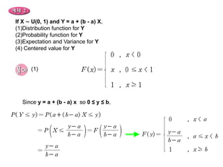
![(Continuous) Uniform Distributions
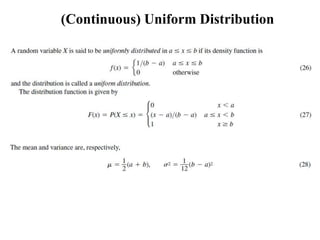
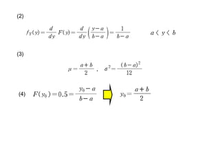
In a Period [a, b], f(x) is constant.
f(x)
E(x):](https://image.slidesharecdn.com/7-121007061603-phpapp01/85/7-16-320.jpg)


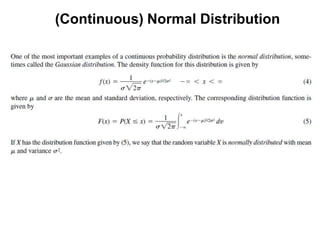
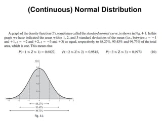
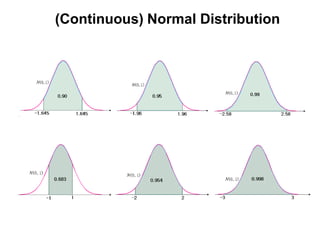
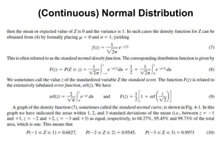
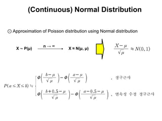
![(Continuous) Normal Distribution
[Ref]
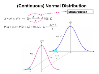
μ is the center of the graph and σ is the degree of variance.
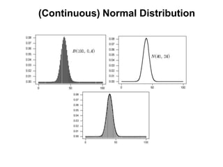
μ is different and σ is same μ is same and σ is different.](https://image.slidesharecdn.com/7-121007061603-phpapp01/85/7-55-320.jpg)
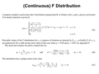

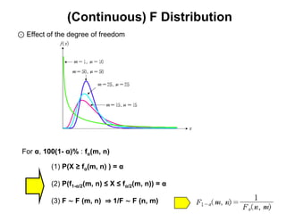
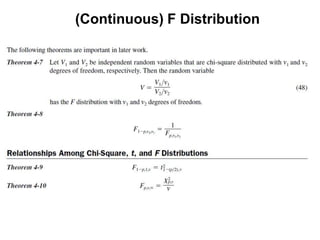
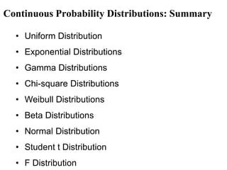

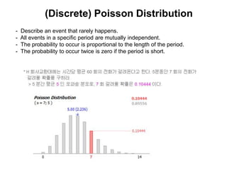
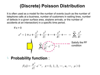
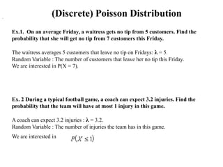
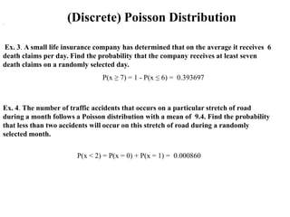
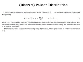
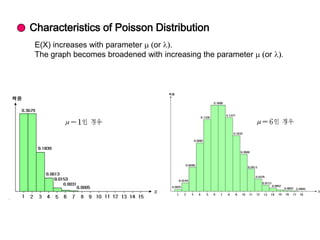
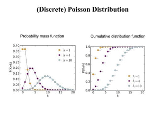
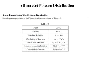
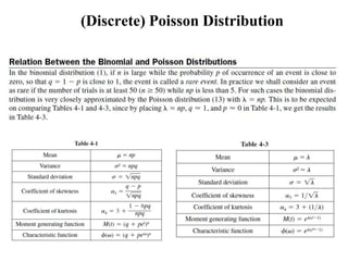
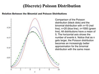
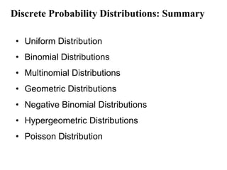
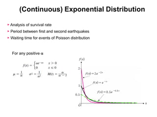
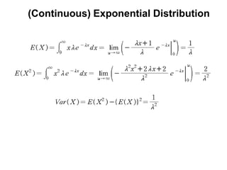
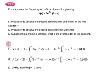
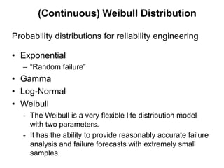
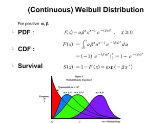
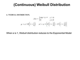
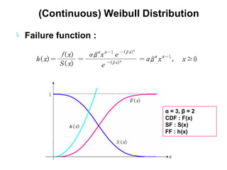
This document provides an overview of the Poisson distribution and other special probability distributions. It discusses: 1) The Poisson distribution and its properties, including how it can model rare, independent events over time periods. Examples of how to calculate probabilities using the Poisson are provided. 2) Other discrete distributions like the binomial, negative binomial, and hypergeometric. 3) Continuous distributions like the uniform, exponential, gamma, chi-square, and Weibull distributions. Applications and properties of each are summarized. 4) Comparisons between distributions like how the Poisson approximates the binomial for large values. Overall, the document introduces several important probability distributions used in statistics.


