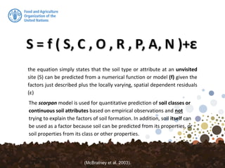
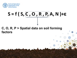
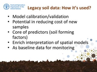
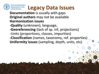
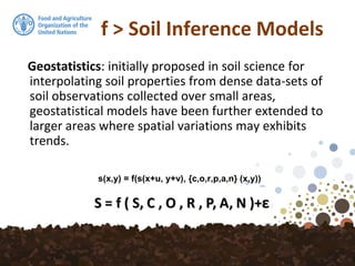
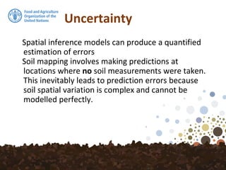
The document discusses Digital Soil Mapping (DSM), detailing its definition, methodologies, and applications in creating digital maps of soil types and properties using various data sources and predictive models. It emphasizes the importance of legacy soil data, climate factors, organisms, relief, and parent material in soil mapping, and outlines the challenges and uncertainties involved in the prediction processes. Additionally, it highlights the integration of various global datasets and modeling techniques that enable effective soil characterization and mapping.

1. Yusuf YIGINI, PhD - FAO, Land and Water Division (CBL)
GSP - Eurasian Soil
Partnership - Dijital
Toprak Haritalama ve
Modelleme Egitimi
Izmir, Turkiye
21-25 Agustos 2017

2. Digital Soil mapping (DSM)

3. What is DSM
What is digital soil mapping?
Also called predictive soil mapping!
The creation and population of spatial soil information
systems by numerical models.
(Lagacherie & McBratney, 2007)

4. What is DSM
What is digital soil mapping?
Digital Soil Mapping also referred to as predictive soil
mapping is the computer-assisted production of digital
maps of soil types and soil properties. Soil mapping, in
general, involves the creation and population of spatial
soil information by the use of field and laboratory
observational methods coupled with spatial and non-
spatial soil inference systems. Digital soil maps are linked
to an underlying digital elevation model whereby grid
cells of the model are populated with soil attributes.

5. (McBratney et al. 2003).
Digital Soil Mapping : The general principle

6. the equation simply states that the soil type or attribute at an unvisited
site (S) can be predicted from a numerical function or model (f) given the
factors just described plus the locally varying, spatial dependent residuals
(ε)
(McBratney et al. 2003).
The scorpan model is used for quantitative prediction of soil classes or
continuous soil attributes based on empirical observations and not
trying to explain the factors of soil formation. In addition, soil itself can
be used as a factor because soil can be predicted from its properties, or
soil properties from its class or other properties.

7. S
Legacy soil data (Soil Samples, Profiles, Soil maps)

8. C, O, R, P > Spatial data on soil forming
factors

9. f > Soil Inference Models

10. S
Legacy soil data (Soil Samples, Profiles, Soil maps)

11. Legacy soil data: How it’s used?
• Model calibration/validation
• Potential in reducing cost of new
samples
• Core of predictors (soil forming
factors)
• Enrich interpretation of spatial models
• As baseline data for monitoring

12. Legacy Data Issues
Documentation is usually with gaps
Original authors may not be available
Harmonization issues
-Quality (unknown), language,
-Georeferencing (lack of sp. inf, projections)
-Units (proportions, classes, impurities)
-Classification (names, taxonomy, ref. properties)
Uniformity issues (sampling, depth, units, etc)

13. Collecting Legacy Soil Data
• All existing soil information collected to
characterise or map soil properties
• landscape and site descriptions,
• Soil profile descriptions
• laboratory analysis (chemical, physical and
biological soil properties)
• Soil Maps
• Soil Sampling Campaigns

14. Collecting Legacy Soil Data
Kingdom of Thailand
General Soil Map.
(North).
(EUDASM)

15. Collecting Legacy Soil Data
(EUDASM)
Author: Soil Survey
Division, Bangkok.
Year: 1979

16. C, O, R, P > Spatial data on soil forming
factors

17. C - Climate
Climate model outputs, National Data, Global
Regional Datasets
Common climatic variables that are regularly
observed and mapped over countries are:
minimum and maximum temperature, cumulated
mean, temperature, mean temperature,
precipitation, potential evapotranspiration,
climatic water balance, global, radiation, snow
depth etc..

18. Global Climate DatasetsWorldClim V1.4 and V2
WorldClim is a set of global climate layers (gridded
climate data) with a spatial resolution of about 1 km2 (10
minutes, 5 minutes, 2.5 minutes are also available).
These data can be used for mapping and spatial
modelling. The current version is Version 1.4. and a
preview of Version 2 is available for testing at
worldclim.org. The data can be downloaded as generic
grids or in ESRI Grid format.

19. O - Organisms
RS Images of Vegetation, Land use/Land Cover

20. O - Organisms
A vegetation index is an indicator that
describes the greenness — the relative density
and health of vegetation — for each pixel, in a
satellite image. Although there are several
vegetation indices, one of the most widely
used is the Normalized Difference Vegetation
Index (NDVI).

21. O - Organisms
Land Cover
Land use and/or land cover data are unarguably
the one of the most vital data for any statistical
effort to map soil properties. There are many of
various sources of data on land cover including
global and continental products, such as
GlobCover, GeoCover, Globeland30, CORINE
Land Cover.

22. O - Organisms
GlobCover
GlobCover is a European Space Agency (ESA) initiative which
began in 2005 in partnership with JRC, EEA, FAO, UNEP, GOFC-
GOLD and IGBP. The aim of the project was to develop a service
capable of delivering global composites and land cover maps using
as input observations from the 300m MERIS sensor on-board the
ENVISAT satellite mission.

23. O - Organisms
Landsat GeoCover
The Landsat GeoCover collection of global
imagery was merged into mosaics by the
Earth Satellite Company (now MDA Federal).
Pixel size: 14.25 meters (V 2000)
The data is available at: ftp://ftp.glcf.umd.edu/glcf/Mosaic_Landsat/ (FTP Access)

24. O - Organisms
Globeland30 (Global)
GlobeLand30, the world’s first global land
cover dataset at 30m resolution for the years
2000 and 2010, was recently released and
made publicly available by China.
The data is publicly available for non-commercial purposes at:
http://www.globallandcover.com/GLC30Download/index.aspx

25. R - Relief
DEM Source Datasets
Currently, two global level 30m DEMs are freely
available; the Shuttle Radar Topographic Mission
(SRTM) and the ASTER Global Digital Elevation
Model (GDEM). They provide topographic data the
global scale, which are freely available for users.

26. R - Relief
● Recommended for national level applications: 30 m GDEM / SRTM
● Recommended for global level applications: SRTM 90m, resampled
1 kilometre.
GDEM / SRTM
In both cases noise and artefacts need to be filtered out. ASTER seems
to contain more large artefacts (e.g. peaks), particularly in flat terrain,
which are very difficult to remove through filtering.

27. R - Relief
GDEM / SRTM
GRASS GIS or GDAL: use "mdenoise" module/utility
to remove noise while preserving sharp features like
ridges, lines and valleys.
SRTM contains many gaps (pixels with no-data).
These gaps could be filled using splines. SAGA GIS
has a module called ‘Close Gaps with Splines’ and
other similar tools for doing this.

28. P - Parent Material, Lithology
National parent material and geology
maps may be used. Other available
datasets and data portals are given on
the ISRIC WorldGrids website
(worldgrids.org).

29. P - Parent Material, Lithology
OneGeology: The world geological maps
are now being integrated via the
OneGeology project which aims at
producing a consistent Geological map
of the world in approximate scale 1:1M
(Jackson, 2007).

30. P - Parent Material, Lithology
USGS has several data portals, e.g. that allow
browsing of the International Surface Geology
(split into South Asia, South America, Iran, Gulf
of Mexico, Former Soviet Union, Europe,
Caribbean, Bangladesh, Asia Pacific, Artic,
Arabian Peninsula, Africa and Afghanistan)
https://mrdata.usgs.gov/geology/world/.

31. P - Parent Material, Lithology
Hartmann and Moosdorf (2012) have assembled
a global, purely lithological database called
GLiM (Global Lithological Map). GLiM consists
of over 1.25 million digital polygons with
classified in three levels (a total of 42 rock-type
classes). https://www.geo.uni-
hamburg.de/en/geologie/forschung/geochemie
/glim.html).

32. P - Parent Material, Lithology
USGS jointly with ESRI has released in 2014 a Global
Ecological Land Units map at 250 m resolution. This
also includes world layer of rock types. This data can
be downloaded from the USGS site
(http://rmgsc.cr.usgs.gov/outgoing/ecosystems/Glo
bal/).

33. f > Soil Inference Models

34. f > Soil Inference Models
Pedometrician
approaches (data-
driven)
Quantitative soil
surveyor
approaches
(knowledge
driven)

35. Conventional Way
The two conventional upscaling methods
(Class-matching,Geomatching), in the
context of SOC mapping, are described
by Lettens et al. (2004).

36. Conventional Way
Details about weighted averaging can be found in
Hiederer (2013).
Different conventional upscaling approaches were
applied in many countries (Baritz et al. 1999
(Germany), Cruz-Gaistardo (Mexico), Greve et al.
2007 (Denmark), Koelli et al. 2009 (Estonia), Arrouay
et al. 2001 (France), Bhatti et al. 2002 (Canada)).

37. Conventional Way
Each approach has been adapted to the structure of
the national soil data bases, information about soil
associations within mapping units, and the degree of
stratification, climatic or eco-regions, land cover
types, and combinations among them.
The core principle is that plot-level soil data are
combined with soil maps via class and geomatching.

38. Conventional Way

39. f > Soil Inference Models
DATA MINING: The most frequently data mining
models used in soil science are multiple regression
(e.g. Moore et al., 1993; Odeh et al., 1994),
classification trees (Bell et al., 1992), and neural
networks (McBratney et al., 2000; Zhu, 2000;
Behrens, 2005). Because they are fully generic,
such models are well documented, largely
implemented in statistical software and possibly
coupled with GIS.
s(x,y) =f({c,o,r,p,a,n}(x,y))
P. Lagacherie SECS10 12.02.2010

40. f > Soil Inference Models
Geostatistics: initially proposed in soil science for
interpolating soil properties from dense data-sets of
soil observations collected over small areas,
geostatistical models have been further extended to
larger areas where spatial variations may exhibits
trends.
s(x,y) = f(s(x+u, y+v), {c,o,r,p,a,n} (x,y))

41. Uncertainty
Spatial inference models can produce a quantified
estimation of errors
Soil mapping involves making predictions at
locations where no soil measurements were taken.
This inevitably leads to prediction errors because
soil spatial variation is complex and cannot be
modelled perfectly.

42. Uncertainty
In fact, we may even be uncertain about the soil at
the measurement locations because no
measurement method is perfect and uncertainty
also arises from measurement errors.

43. DigitalSoilMappingWorkflow
Dobos, E., Carré,
F., Hengl, T.,
Reuter, H.I., Tóth,

45. Next: Working with R, R Studio: Basics