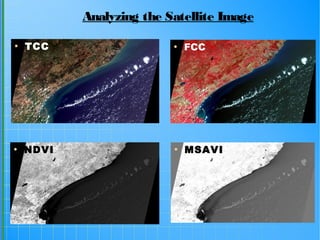
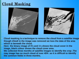
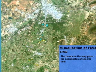
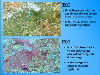
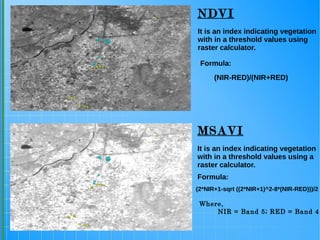
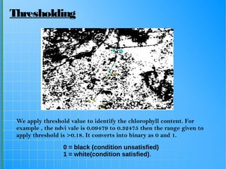
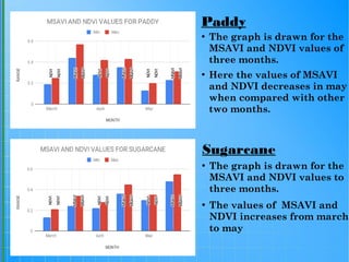
Geo spatial technologies can be used to identify crop fields using satellite imagery. Data is collected using satellite images and GPS coordinates of fields. Images are analyzed using techniques like cloud masking, true/false color composites, NDVI, and MSAVI to understand vegetation levels. Thresholding is applied to NDVI and MSAVI values to identify areas as paddy or sugarcane fields. Graphs show the crops' values decrease or increase over months in ways that can distinguish between them. Crop identification through geo spatial analysis is faster and cheaper than field surveys, and helps estimate crop areas for agricultural decision making.

1. GEOSPATIAL TECHNOLOGIES
FOR
CROP IDENTIFICATION
Identify your crop using GIS

2. ●
Introduction
●
Cloud Masking
●
Data Collection
●
Visualization of Field Crop
●
TCC and FCC
●
NDVI and MSAVI
●
Thresholding
●
Graph
INDEX

3. ● “Geo Spatial Analysis” covers a wide range of techniques to
analyze spatial data.
● We are assessing how Geo Spatial techniques are utilized
for identification of the crop field.
● The ability to identify crop type makes it possible to
estimate the area allocated to each crop type and thus
compute relevant statistics providing essential information.
● Accurate and faster estimation of crop area is very essential
for projecting yearly agriculture and deciding agriculture
policies.
● Here, We try to analyze and identify the difference between
paddy and sugarcane crops.
Introduction

4. Data Collection
● To solve the problems in targeted fields we collect data
(information) of the field.
● we downloaded three months of LANSAT8(OLI) satellite images
from earth explorer in the purpose of gathering data and tried to
identify features in the image.
● We selected Anakapalle as our field area to collect the data
● With the help of an Android app KRITI DEMO we collected some
points of the field at a distance of 100 meters each and the app
records the coordinates of that points using GPS.
● we used open source GIS tools (QGIS) for getting the values of
chlorophyll of three months of the gathered points by performing
(TCC, FCC, NDVI and MSAVI) in order to understand vegetation
area.
● The data in the app is in .CSV format which we add as delineate
layer in Qgis for plotting the points on the image.

5. Analyzing the Satellite Image
●
TCC ●
FCC
●
MSAVI●
NDVI

6. Cloud Masking
● Cloud masking is a technique to remove the cloud from a satellite image
though cloud in the image was removed we loss the data of the area
which is beneath the cloud.
● Here the binary image of 0's and 1's shows the cloud cover in the
image, black colour shows the cloud cover area.
● We collected three months of satellite images to identify the crop .The
may image has so much cloud of over 45% so it is difficult to identify
the common fields in three months.

7. Visualization of Field
crop
The points on the map gives
the coordinates of specific
field

8. ● By adding bands 4,3,2 we
can observe the true colour
composite of the image.
●
In this image green colour
represents vegetation.
● By adding bands 5,4,3
we can observe the
false colour composite
of the image.
● In this image red
colour represents
vegetation.
TCC
FCC

9. It is an index indicating vegetation
with in a threshold values using a
raster calculator.
It is an index indicating vegetation
with in a threshold values using
raster calculator.
NDVI
MSAVI
(2*NIR+1-sqrt ((2*NIR+1)^2-8*(NIR-RED)))/2
Formula:
Where,
NIR = Band 5; RED = Band 4
Formula:
(NIR-RED)/(NIR+RED)

10. We apply threshold value to identify the chlorophyll content. For
example , the ndvi vale is 0.09479 to 0.32475 then the range given to
apply threshold is >0.18. It converts into binary as 0 and 1.
0 = black (condition unsatisfied)
1 = white(condition satisfied).
Thresholding

11. Paddy
●
The graph is drawn for the
MSAVI and NDVI values of
three months.
●
Here the values of MSAVI
and NDVI decreases in may
when compared with other
two months.
Sugarcane
●
The graph is drawn for the
MSAVI and NDVI values to
three months.
●
The values of MSAVI and
NDVI increases from march
to may

12. ● Crop identification through ground
surveys are expensive and yet cover only
a sample of farms. Where as Geo Spatial
Analysis covers a wide range of
techniques which are used in identifying
the crops in spatial data and it is faster
and cheaper. Accurate and faster
estimation of crop area is very essential
for area-based subsidies and helps in
deciding agriculture policies.
CONCLUSION

13. Thank You
ACKNOWLEDGEMENT
● In this project, we used open source software QGIS
(https://qgis.org/) and satellite images of March, April, and May
2018 from NASA’s USGS portal (https://earthexplorer.usgs.gov/)
● Thank you KAIINOS (https://www.kaiinos.com/) for your support
and guidance in completion of our project.
Sai Kiran: http://www.linkedin.com/in/godi-saikiran
Komali: http://www.linkedin.com/in/komaliavirneni
Krishna: http://linkedin.com/in/krishnacheekatla