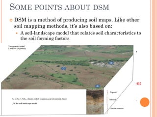
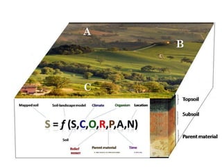
The document outlines a comprehensive digital soil mapping (DSM) capacity-building course, focusing on theoretical knowledge and practical skills for soil scientists over a week-long intensive training. It includes topics such as input data requirements, documentation in MS Word, and different DSM methods and tools, as well as opportunities for hands-on practice and case studies using personal datasets. By the end of the course, participants are expected to effectively compile data, use various software for DSM, and develop accurate digital soil maps for national soil information systems.

1. DIGITAL SOIL MAPPING – CAPACITY
BUILDING COURSE
Day 2

2. COURSE PLAN
1 week intensive training
 Theory– Introduction, basics, procedures
 Practical – hands-on practice
 Assignments
 Half-day– discussion on problems encountered
Case-study
 Development of case studies
 Practical application on own dataset
 Presentation of case-studies,
 Final evaluation

3. COURSE AIMS
To equip soil scientists/staff at national
institutions with recent techniques in DSM.
 Exposure to recent developments in DSM methods and
tools for developing and updating national and
regional soil information.
 Practical orientation to give opportunity to implement
the DSM techniques
 Allow simultaneous use of own data to develop
relevant DSM products
 Support update of soil information

4. COURSE OUTCOMES
To be able to:
 Compile and harmonize legacy data and other
input data for DSM applications
 Use various software to implement DSM
 Develop accurate digital soil maps for updating
national soil information systems

5. COURSE STRUCTURE
 Lectures
 Discussions and clarifications
 Practical sessions
 Demonstrations
 Hands-on exercises
 Assignments
 Follow-up work
 Case study
 Individual work
 Own case study
 Plenary discussions
 Group discussion
 Individual presentations

6. OBJECTIVES FOR DAY 2
 To expose participants to the theory and
principles of DSM
 To introduce DSM input requirements
 To familiarize participants with documentation
steps and DSM methods

7. HOW TO BEGIN DOCUMENTATION IN MS WORD
 Documenting steps
 Open new word document
 Put the requisite headings and explanations
 Add images from the computer using: Alt+PrtSc etc.
 Save the document
 Documenting data information (metadata)
 Data type
 Data source (author, website, copyright, format)
 Data characteristics (number, projection, formula,
etc.)
 Date (of creating or access)
 Save metadata in the same folder as the data

8. SOME POINTS ABOUT DSM
 DSM is a method of producing soil maps. Like other
soil mapping methods, it’s also based on:
 A soil-landscape model that relates soil characteristics to
the soil forming factors
 Computer applications to implement the soil landscape
model (difference being - heavy dependency )
 GIS layers of soil forming factors as input to the model
 In addition; Mathematical/statistical models to represent
the soil-landscape model
 Defined simply as computer-assisted production of
digital maps of soil

9. MISCONCEPTIONS ABOUT DSM
 No need for field sampling (i.e. Remote Sensing is
adequate) ----NOT TRUE
 It relies much on adequately sampled soil data as input
 Field validation is an integral component of DSM
 Geo-referencing and local knowledge are assets in DSM
 Computer does all the mapping----NOT TRUE
 Computing is a core method/tool in DSM
 Computing cannot replace soil profile description
and laboratory analysis – steps in soil mapping
 It’s replacing basic soil science----NOT TRUE
 Soil science is the foundation
 DSM enriches approaches to soil mapping
 There are still needs for all soil mapping products

10. HOW DOES DSM WORK
 The principles
 Soil formation and distribution is influenced by
 Climate, organisms, topography, parent materials, time
 If spatial distribution of these factors is known then soil
character may be inferred
 Soil character may not always show hard boundaries
between differing and contiguous groups
 Ordering of soil character in the landscape is not
arbitrary – there is a law obeyed/pattern followed
 These principles have been employed for ages in
soil mapping albeit with varied success
 They have been combined to lay ground for
development of operating guidelines in DSM

11. DSM THEORY
 Spatial distribution of soil forming factors is a function
of magnitude and spatial distribution of soil forming
factors
 Theory can be mathematically modelled
 There exists a quantifiable/hueristic function f to link
the SCORPAN factors and soil character
 If the function is applied at known/sample locations
and quantities, then it can be used to predict the soil
attribute at unknown/un-sampled locations
A
B
C

12. STEPS IN DSM
 Three major stages: input data, tools and
methods selection, and soil information system
Legacy soil data
• Soil sampling/survey
• Secondary data
Environmental factors/GIS
database
• Remote sensing images
• DEM
• Land use/cover
• Climate data
• Geology maps
Digital soil assessments
Uncertainties of spatial
prediction
DSM Methods
DSM Tools
GIS layers of soil
Properties and types
Expert/technical support
• Scientists
• Technicians
• Soil information users
• Technical manual
• Standards
Stage I
Input
Stage II
Tools and method selection
Stage III
Soil information system
Spatial database / soil
information system
Soil inference system

13. INTRODUCTION TO DSM INPUT
REQUIREMENTS

14. INPUT 1: DATA
 Input data requirements
 Existing soil maps
 Soil profile data
 Lab analytical and field observation soil data
 Climate data
 Other maps – Altitude, Geology, Land use/cover
 Typical sources of input DSM data
Input data Source Level of detail (Resolution)
< 20 m 20 – 200 m > 200 m
Land use/ land cover Multi spectral remote
sensing images
GeoEye, Quickbird,
Ikonos, SPOT
Landsat,
ASTER,
MODIS, AVHRR,
MERIS
Hyper-spectral remote
sensing images
AVIRIS
Radar, radiometry LIDAR ASAR, MWR
Vegetation/land cover GLOBCOVER
Relief DEM National Contour
or Topomaps
ASTER, SRTM GTOPO
Climate Climate (rainfall) data National archives MARS, AVHRR
Parent material Geology maps National archives
Geological surveys Regional studies Gamma –ray
spectrometry
Global geology
map
Soil Soil profile/properties Regional soil
surveys
National, ISRIC, FAO
Soil maps Regional soil maps

15. INPUT 2: DSM METHODS
 Spatial interpolation
 To make smooth trend over discrete locations
 Digital terrain models
 To derive relief characteristics
 Remote sensing analysis
 To extract land use and land cover characteristics
 Statistical modelling
 To explore and understand data characteristics
 To model relationships
 To quantify confidence in inputs and outputs

16. DSM TOOLS AND SOFTWARE
Method Tools Software
Spatial interpolation
Geostatistics R
Non-geostatistical method QGIS, ILWIS
Terrain analysis Digital Terrain modelling SAGA, QGIS
Remote sensing analysis
Image correction ILWIS, QGIS
Image Indices ILWIS
Classification ILWIS
Statistical analysis
Multivariate analysis ILWIS, R
Correlation analysis R
Database management
Storage MS Office
Dissemination Google Earth

17. LEGACY DATA
 All existing soil information collected to
characterize or map soils
 landscape and site descriptions,
 soil profile morphological descriptions
 laboratory analysis of the main chemical, physical and
biological soil properties
 Soil maps
 Geophysical/geotechnical surveys
 Other maps – climate, geology, land use, contour
and topographic maps
 Tacit knowledge - reports, legends, mental
models

18. IMPORTANCE OF LEGACY DATA
Model calibration/validation
Potential in reducing cost of new samples
Core of predictors (soil forming factors)
Enrich interpretation of spatial models
As baseline data for monitoring
Input into SCORPAN modelling

19. PROBLEMS WITH LEGACY DATA
 Documentation is usually with gaps
 Original authors may not be available
 Harmonization issues
 Quality (error), language,
 Georeferencing (lack/un-clear/diff. projection)
 Map units (proportions, classes, impurities)
 Classification (names, taxonomy, ref. properties)
 Uniformity issues (sampling, depth, units, etc)

20. DSM TOOLS AND METHODS

21. DATABASE DEVELOPMENT
 The core of DSM
 Features
 It should be user friendly
 It should contain adequate information
 Amenable to DSM software
 Software
 MS Office
 QGIS
 ILWIS

22. OBTAINING DSM DATA
 Clarify what is to be done (Map properties/classes)
 Specify type of data needed
 Identify sources and summarize data availability
 Document available data and check for gaps
 Obtain the data
Data Type Source
Soil Soil profiles ISRIC (http://www.isric.org/data/isric-wise-global-soil-profile-data-ver-31)
Soil maps UN-FAO (http://www.fao.org/soils-portal/soil-survey/soil-maps-and-
databases/soil-profile-databases/en/)
IIASA
(http://www.iiasa.ac.at/web/home/research/modelsData/HWSD/HWSD.en.html)
Soil legacy reports FAO (http://www.fao.org/soils-portal/soil-survey/soil-maps-and-databases/soil-
legacy-reports/en/)
Laboratory
analytical data
National soil laboratories, research institutes (e.g. NGOs, Universities, etc)
Remote
sensing image
MODIS NDVI (250 m) USDA (http://pekko.geog.umd.edu/usda/apps/)
Land cover (300 m) ESA (http://due.esrin.esa.int/globcover/)
Landsat (30 m) GLCF (http://glcf.umd.edu/data/)
Cover (< 30 m) National aerial photo missions
DEM SRTM (90 m) http://srtm.usgs.gov/ or http://lta.cr.usgs.gov/
ASTER (30 m) http://asterweb.jpl.nasa.gov/gdem.asp or http://lta.cr.usgs.gov/
DEM (<30 m) National contour maps
Geology 1:1 M National geologic maps
> 1:1 M Sub-regional (sub-national) geologic maps
Climate Rainfall National meteorological departments
Create DSM workspace
 C:DSM - where we will work
 C:DSMInput - where to keep input data
 C:DSMOutput - where to keep output data

23. DOWNLOAD ONLINE SOIL MAP
http://esdac.jrc.ec.europa.eu
/resource-type/maps

25. SCANNED SOIL MAP
Legend

26. GETTING DEM FROM ONLINE ARCHIVE
https://lta.cr.usgs.gov/

28. DOWNLOAD SOIL PROFILES FROM
ISRIC
http://www.isric.org/data/
isric-wise-global-soil-
profile-data-ver-31

29. OBTAINING DATA FROM ISRIC
Example

30. DOWNLOAD LAND COVER FROM
ONLINE ARCHIVE
http://due.esrin.esa.int
/page_globcover.php

32. EXAMPLE: 300 M LAND COVER (2009)

33. MODIS WEBSITE
http://pekko.geog.umd.edu/
usda/test/

34. EXAMPLE: DOWNLOADING MODIS

35. Which soil data is available
Which environmental covariate is
available
Detailed soil map with
Legends and soil data
Soil point data with site
description
Detailed soil map
with legend
No data
All covariates
C, O, R, P
At least 3 covariates
Including R & O
At least 2 covariates
Including R
Only one covariate No data
Increasing level of data inadequacy
Climate (C)
Organism (O)
Relief (R)
Parent (P)
Relief (R)
Organism (O)
Relief (R)
Climate – mean rainfall (map or weather station data)
Organism – Land use/land cover
Relief – Elevation map (DEM)
Parent – Geology map
Soil – georeferenced soil properties, profile, map

36. Data Type Number Source
DEVELOPING METADATA

37. ASSIGNMENT: BUILDING GEO-DATABASE
FOR DSM APPLICATION-STEP 1
 Use your own data/obtain from online data archives
 Explore the data
 Document the characteristics of the data:
 Source and author of data
 Data type (profile, analytical, georeferenced, maps, etc.)
 Number of samples/cases
 Use the table format (use Data, Type, Number, Source, as column
heading)
 Save the database & documentation (C:DSMInput)