This document discusses production and cost analysis concepts from a managerial economics textbook chapter. It defines key terms like total, average and marginal product, isoquants, isocosts, and different cost functions. It explains how firms determine optimal input levels by equalizing the value of marginal products with input prices to minimize costs. Firms produce at the point where the marginal rate of technical substitution equals the input price ratio. Cost functions are important for analyzing profit-maximizing behavior.

1. Copyright © 2010 by the McGraw-Hill Companies, Inc. All rights reserved.
McGraw-Hill/Irwin
Managerial Economics & Business
Strategy
Chapter 5
The Production
Process and Costs

2. 5-2
Overview
I. Production Analysis
– Total Product, Marginal Product, Average Product.
– Isoquants.
– Isocosts.
– Cost Minimization
II. Cost Analysis
– Total Cost, Variable Cost, Fixed Costs.
– Cubic Cost Function.
– Cost Relations.
III. Multi-Product Cost Functions

3. 5-3
Production Analysis
Production Function
– Q = F(K,L)
• Q is quantity of output produced.
• K is capital input.
• L is labor input.
• F is a functional form relating the inputs to output.
– The maximum amount of output that can be
produced with K units of capital and L units of
labor.
Short-Run vs. Long-Run Decisions
Fixed vs. Variable Inputs

4. 5-4
Production Function Algebraic
Forms
Linear production function: inputs are perfect
substitutes.
Leontief production function: inputs are used in
fixed proportions.
Cobb-Douglas production function: inputs have
a degree of substitutability.
( ) b
a
L
K
L
K
F
Q =
= ,
( ) bL
aK
L
K
F
Q +
=
= ,
( ) { }
cL
bK
L
K
F
Q ,
min
, =
=

5. 5-5
Productivity Measures:
Total Product
Total Product (TP): maximum output produced
with given amounts of inputs.
Example: Cobb-Douglas Production Function:
Q = F(K,L) = K.5 L.5
– K is fixed at 16 units.
– Short run Cobb-Douglass production function:
Q = (16).5 L.5 = 4 L.5
– Total Product when 100 units of labor are used?
Q = 4 (100).5 = 4(10) = 40 units

6. 5-6
Productivity Measures: Average
Product of an Input
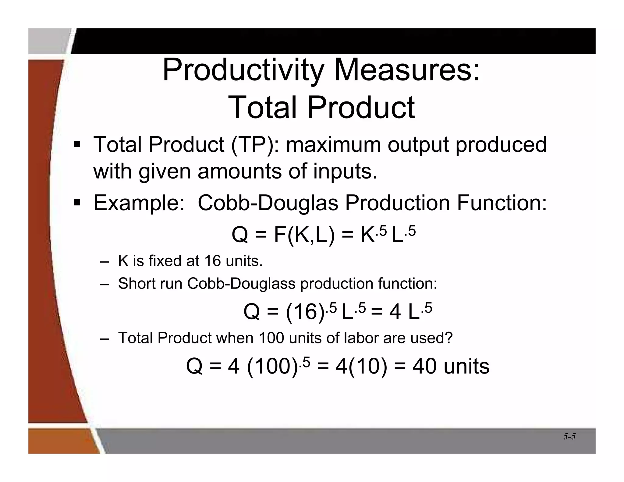
Average Product of an Input: measure of output
produced per unit of input.
– Average Product of Labor: APL = Q/L.
• Measures the output of an “average” worker.
• Example: Q = F(K,L) = K.5 L.5
If the inputs are K = 16 and L = 16, then the average product of
labor is APL = [(16) 0.5(16)0.5]/16 = 1.
– Average Product of Capital: APK = Q/K.
• Measures the output of an “average” unit of capital.
• Example: Q = F(K,L) = K.5 L.5
If the inputs are K = 16 and L = 16, then the average product of
capital is APK = [(16)0.5(16)0.5]/16 = 1.

7. 5-7
Productivity Measures: Marginal
Product of an Input
Marginal Product on an Input: change in total
output attributable to the last unit of an input.
– Marginal Product of Labor: MPL = ∆Q/∆L
• Measures the output produced by the last worker.
• Slope of the short-run production function (with respect to
labor).
– Marginal Product of Capital: MPK = ∆Q/∆K
• Measures the output produced by the last unit of capital.
• When capital is allowed to vary in the short run, MPK is
the slope of the production function (with respect to
capital).

8. 5-8
Q
L
Q=F(K,L)
Increasing
Marginal
Returns
Diminishing
Marginal
Returns
Negative
Marginal
Returns
MP
AP
Increasing, Diminishing and
Negative Marginal Returns

9. 5-9
Guiding the Production Process
Producing on the production function
– Aligning incentives to induce maximum worker
effort.
Employing the right level of inputs
– When labor or capital vary in the short run, to
maximize profit a manager will hire:
• labor until the value of marginal product of labor equals
the wage: VMPL = w, where VMPL = P x MPL.
• capital until the value of marginal product of capital
equals the rental rate: VMPK = r, where VMPK = P x
MPK .

10. 5-10
Isoquant
Illustrates the long-run combinations of
inputs (K, L) that yield the producer the
same level of output.
The shape of an isoquant reflects the
ease with which a producer can
substitute among inputs while
maintaining the same level of output.

11. 5-11
Marginal Rate of Technical
Substitution (MRTS)
The rate at which two inputs are
substituted while maintaining the same
output level.
K
L
KL
MP
MP
MRTS =

12. 5-12
Linear Isoquants
Capital and labor
are perfect
substitutes
– Q = aK + bL
– MRTSKL = b/a
– Linear isoquants imply
that inputs are
substituted at a constant
rate, independent of the
input levels employed. Q3
Q2
Q1
Increasing
Output
L
K

13. 5-13
Leontief Isoquants
Capital and labor are
perfect complements.
Capital and labor are used
in fixed-proportions.
Q = min {bK, cL}
Since capital and labor are
consumed in fixed
proportions there is no
input substitution along
isoquants (hence, no
MRTSKL).
Q3
Q2
Q1
K
Increasing
Output
L

14. 5-14
Cobb-Douglas Isoquants
Inputs are not perfectly
substitutable.
Diminishing marginal
rate of technical
substitution.
– As less of one input is used
in the production process,
increasingly more of the
other input must be
employed to produce the
same output level.
Q = KaLb
MRTSKL = MPL/MPK
Q1
Q2
Q3
K
L
Increasing
Output

15. 5-15
Isocost
The combinations of inputs
that produce a given level of
output at the same cost:
wL + rK = C
Rearranging,
K= (1/r)C - (w/r)L
For given input prices,
isocosts farther from the
origin are associated with
higher costs.
Changes in input prices
change the slope of the
isocost line.
K
L
C1
L
K
New Isocost Line for
a decrease in the
wage (price of labor:
w0 w1).
C1/r
C1/w
C0
C0/w
C0/r
C/w0
C/w1
C/r
New Isocost Line
associated with higher
costs (C0 C1).

16. 5-16
Cost Minimization
Marginal product per dollar spent should be
equal for all inputs:
But, this is just
r
w
MP
MP
r
MP
w
MP
K
L
K
L
=
⇔
=
r
w
MRTSKL =

17. 5-17
Cost Minimization
Q
L
K
Point of Cost
Minimization
Slope of Isocost
=
Slope of Isoquant

18. 5-18
Optimal Input Substitution
A firm initially produces Q0
by employing the
combination of inputs
represented by point A at a
cost of C0.
Suppose w0 falls to w1.
– The isocost curve rotates
counterclockwise; which
represents the same cost
level prior to the wage
change.
– To produce the same level of
output, Q0, the firm will
produce on a lower isocost
line (C1) at a point B.
– The slope of the new isocost
line represents the lower
wage relative to the rental
rate of capital.
Q0
0
A
L
K
C0/w1
C0/w0
C1/w1
L0
L1
K0
K1
B

19. 5-19
Cost Analysis
Types of Costs
– Short-Run
• Fixed costs (FC)
• Sunk costs
• Short-run variable
costs (VC)
• Short-run total costs
(TC)
– Long-Run
• All costs are
variable
• No fixed costs

20. 5-20
Total and Variable Costs
C(Q): Minimum total cost of
producing alternative levels
of output:
C(Q) = VC(Q) + FC
VC(Q): Costs that vary with
output.
FC: Costs that do not vary
with output.
$
Q
C(Q) = VC + FC
VC(Q)
FC
0

21. 5-21
Fixed and Sunk Costs
FC: Costs that do not
change as output changes.
Sunk Cost: A cost that is
forever lost after it has been
paid.
Decision makers should
ignore sunk costs to
maximize profit or minimize
losses
$
Q
FC
C(Q) = VC + FC
VC(Q)

22. 5-22
Some Definitions
Average Total Cost
ATC = AVC + AFC
ATC = C(Q)/Q
Average Variable Cost
AVC = VC(Q)/Q
Average Fixed Cost
AFC = FC/Q
Marginal Cost
MC = DC/DQ
$
Q
ATC
AVC
AFC
MC
MR

23. 5-23
Fixed Cost
$
Q
ATC
AVC
MC
ATC
AVC
Q0
AFC Fixed Cost
Q0×(ATC-AVC)
= Q0× AFC
= Q0×(FC/ Q0)
= FC

24. 5-24
Variable Cost
$
Q
ATC
AVC
MC
AVC
Variable Cost
Q0
Q0×AVC
= Q0×[VC(Q0)/ Q0]
= VC(Q0)
Minimum of AVC

25. 5-25
$
Q
ATC
AVC
MC
ATC
Total Cost
Q0
Q0×ATC
= Q0×[C(Q0)/ Q0]
= C(Q0)
Total Cost
Minimum of ATC

26. 5-26
Cubic Cost Function
C(Q) = f + a Q + b Q2 + cQ3
Marginal Cost?
– Memorize:
MC(Q) = a + 2bQ + 3cQ2
– Calculus:
dC/dQ = a + 2bQ + 3cQ2

27. 5-27
An Example
– Total Cost: C(Q) = 10 + Q + Q2
– Variable cost function:
VC(Q) = Q + Q2
– Variable cost of producing 2 units:
VC(2) = 2 + (2)2 = 6
– Fixed costs:
FC = 10
– Marginal cost function:
MC(Q) = 1 + 2Q
– Marginal cost of producing 2 units:
MC(2) = 1 + 2(2) = 5

28. 5-28
Long-Run Average Costs
LRAC
$
Q
Economies
of Scale
Diseconomies
of Scale
Q*

29. 5-29
Multi-Product Cost Function
C(Q1, Q2): Cost of jointly producing two
outputs.
General function form:
( ) 2
2
2
1
2
1
2
1, cQ
bQ
Q
aQ
f
Q
Q
C +
+
+
=

30. 5-30
Economies of Scope
C(Q1, 0) + C(0, Q2) C(Q1, Q2).
– It is cheaper to produce the two outputs jointly
instead of separately.
Example:
– It is cheaper for Time-Warner to produce
Internet connections and Instant Messaging
services jointly than separately.

31. 5-31
Cost Complementarity
The marginal cost of producing good 1
declines as more of good two is produced:
∆MC1(Q1,Q2) /∆Q2 0.
Example:
– Cow hides and steaks.

32. 5-32
Quadratic Multi-Product Cost
Function
C(Q1, Q2) = f + aQ1Q2 + (Q1 )2 + (Q2 )2
MC1(Q1, Q2) = aQ2 + 2Q1
MC2(Q1, Q2) = aQ1 + 2Q2
Cost complementarity: a 0
Economies of scope: f aQ1Q2
C(Q1 ,0) + C(0, Q2 ) = f + (Q1 )2 + f + (Q2)2
C(Q1, Q2) = f + aQ1Q2 + (Q1 )2 + (Q2 )2
f aQ1Q2: Joint production is cheaper

33. 5-33
A Numerical Example:
C(Q1, Q2) = 90 - 2Q1Q2 + (Q1 )2 + (Q2 )2
Cost Complementarity?
Yes, since a = -2 0
MC1(Q1, Q2) = -2Q2 + 2Q1
Economies of Scope?
Yes, since 90 -2Q1Q2

34. 5-34
Conclusion
To maximize profits (minimize costs)
managers must use inputs such that the
value of marginal of each input reflects price
the firm must pay to employ the input.
The optimal mix of inputs is achieved when
the MRTSKL = (w/r).
Cost functions are the foundation for helping
to determine profit-maximizing behavior in
future chapters.