Cost Analysis for MBA Students

1. Cost &
Production
Analysis

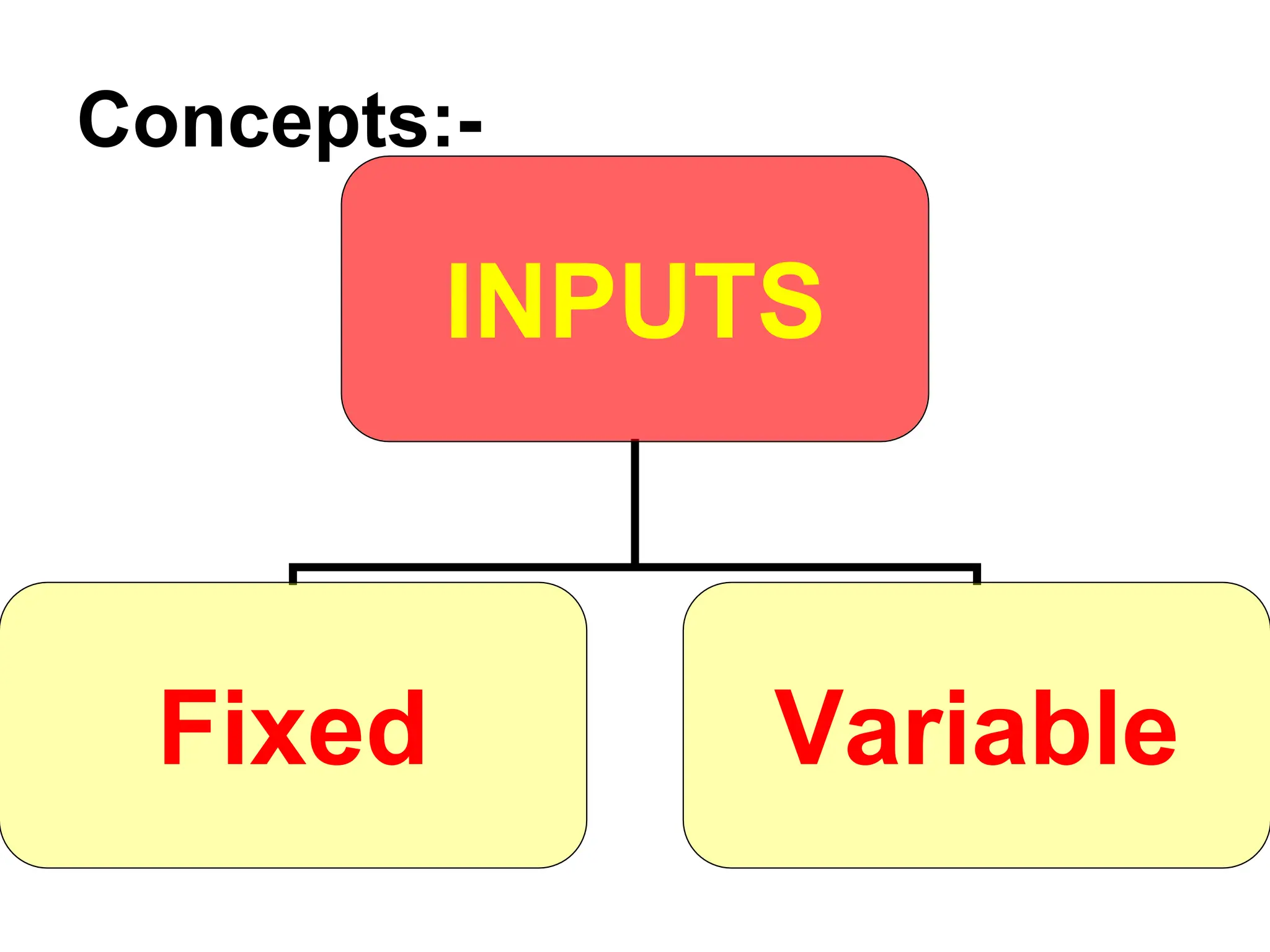
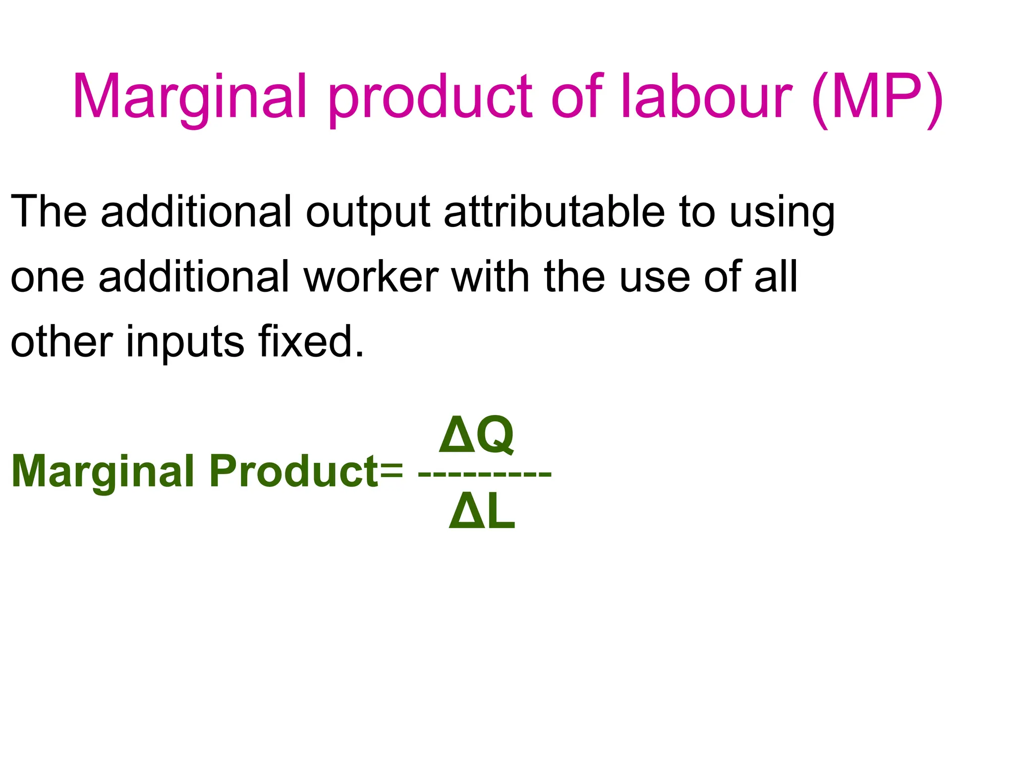
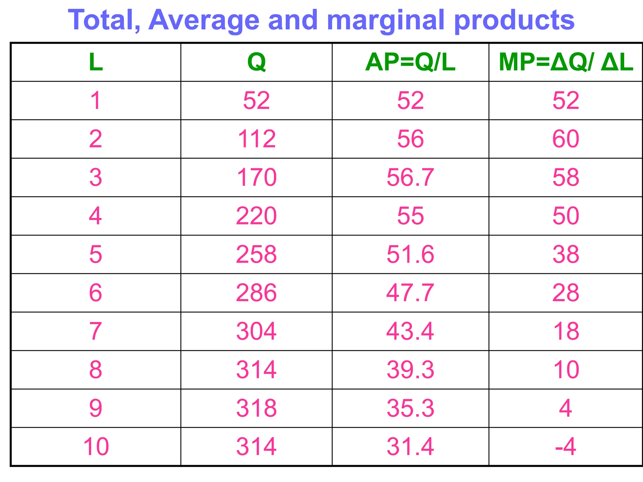
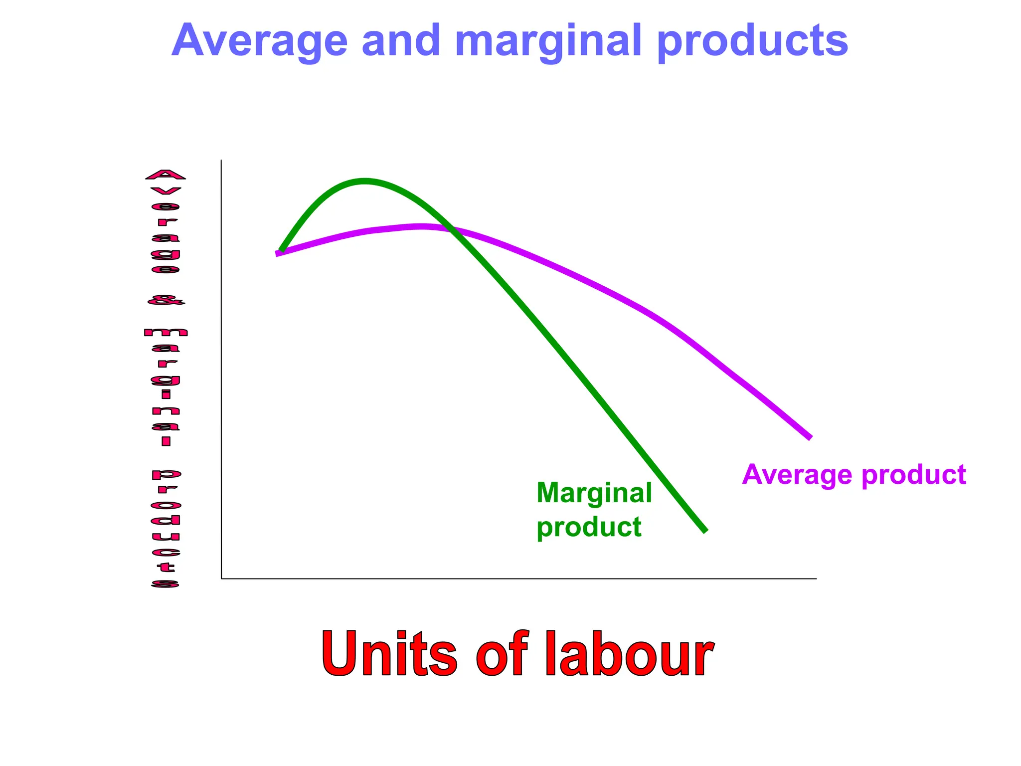
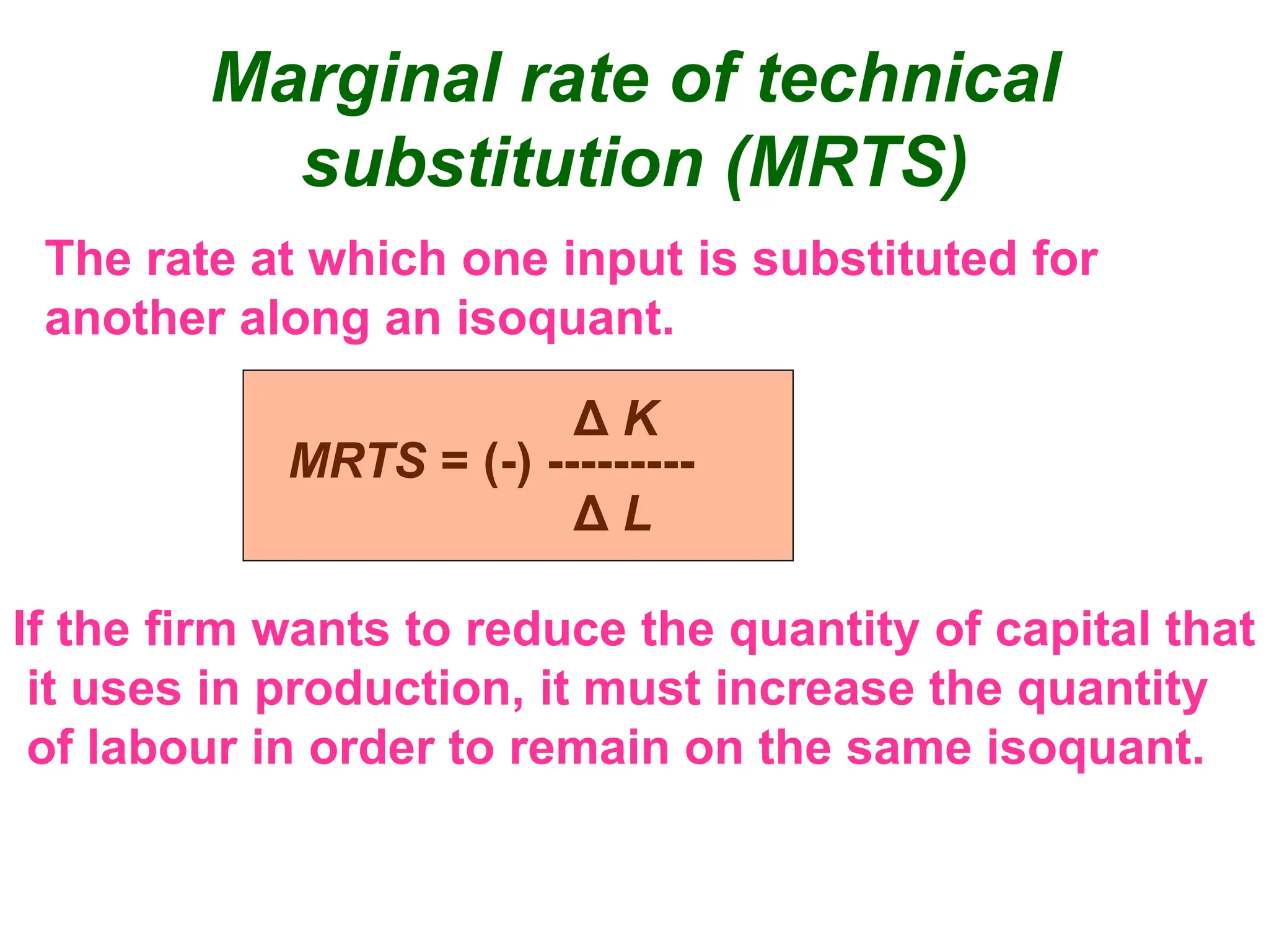
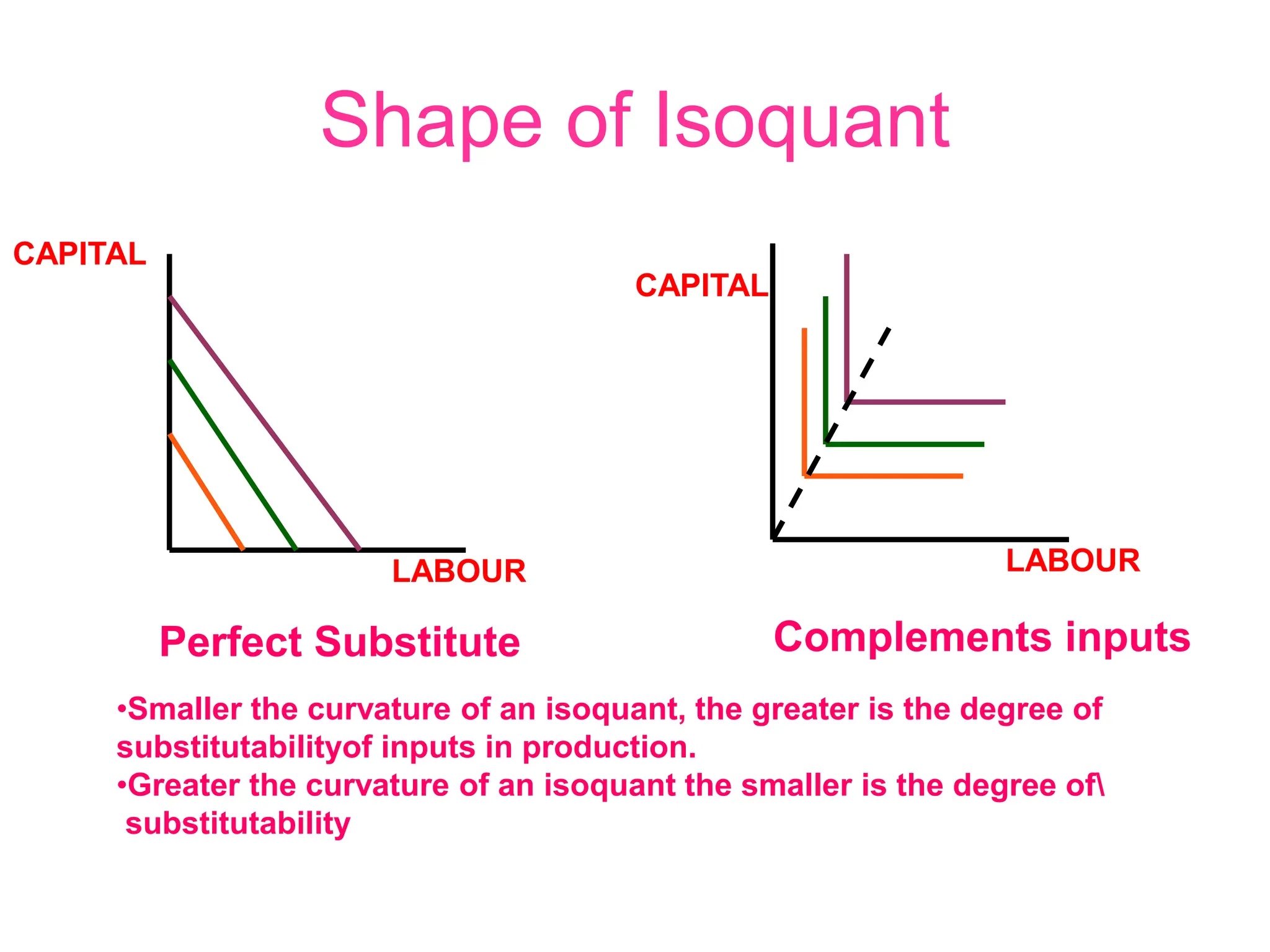
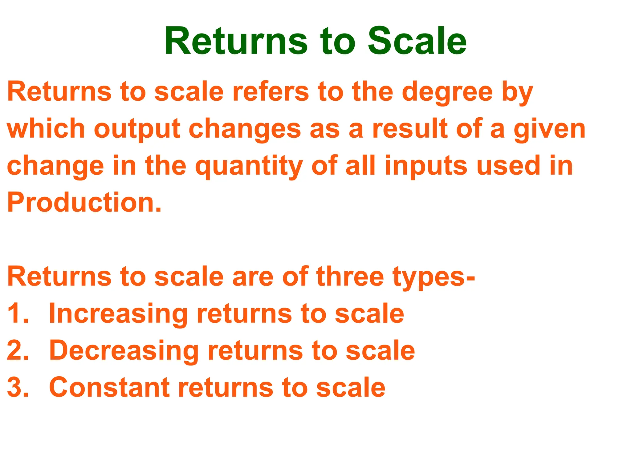
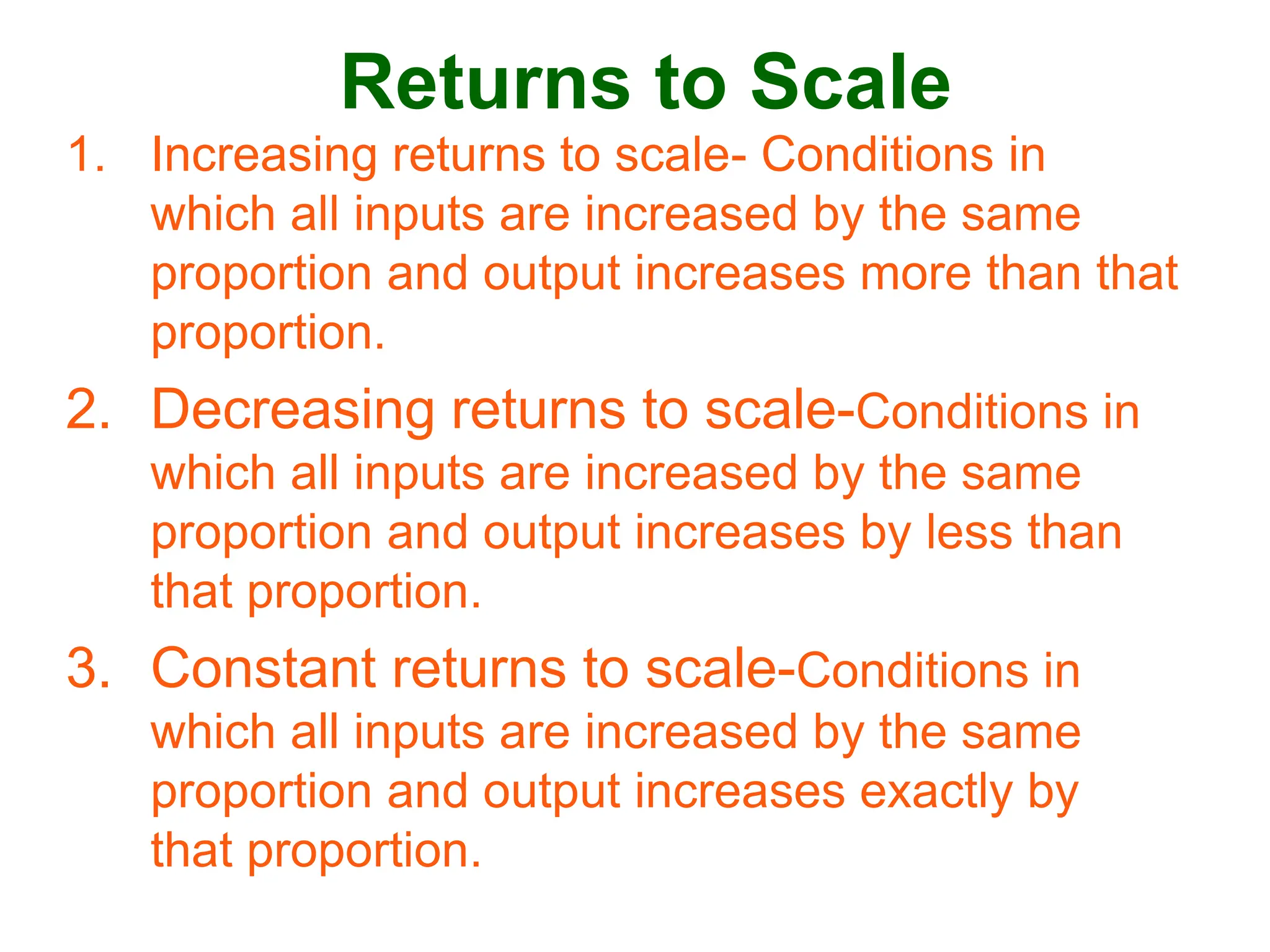
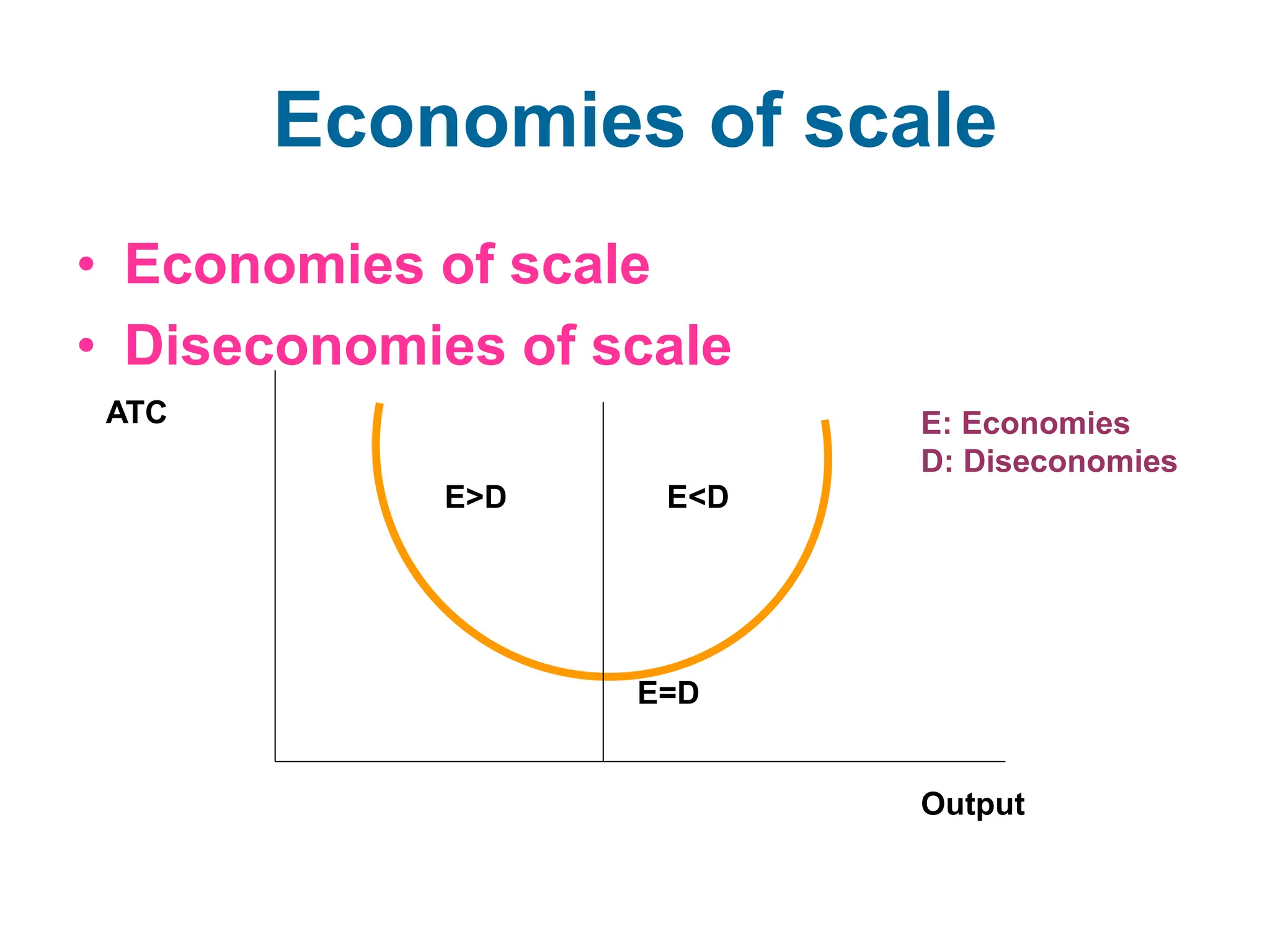
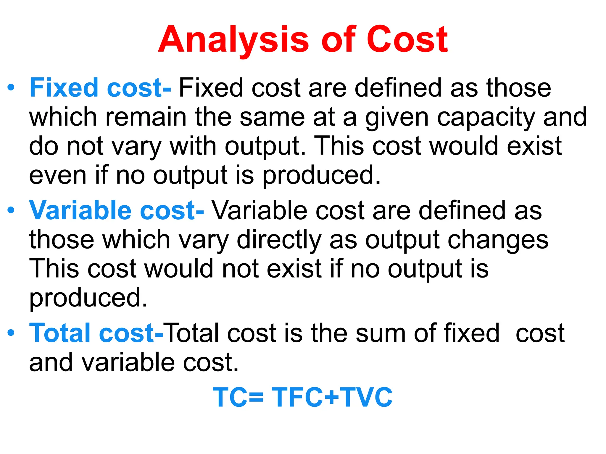
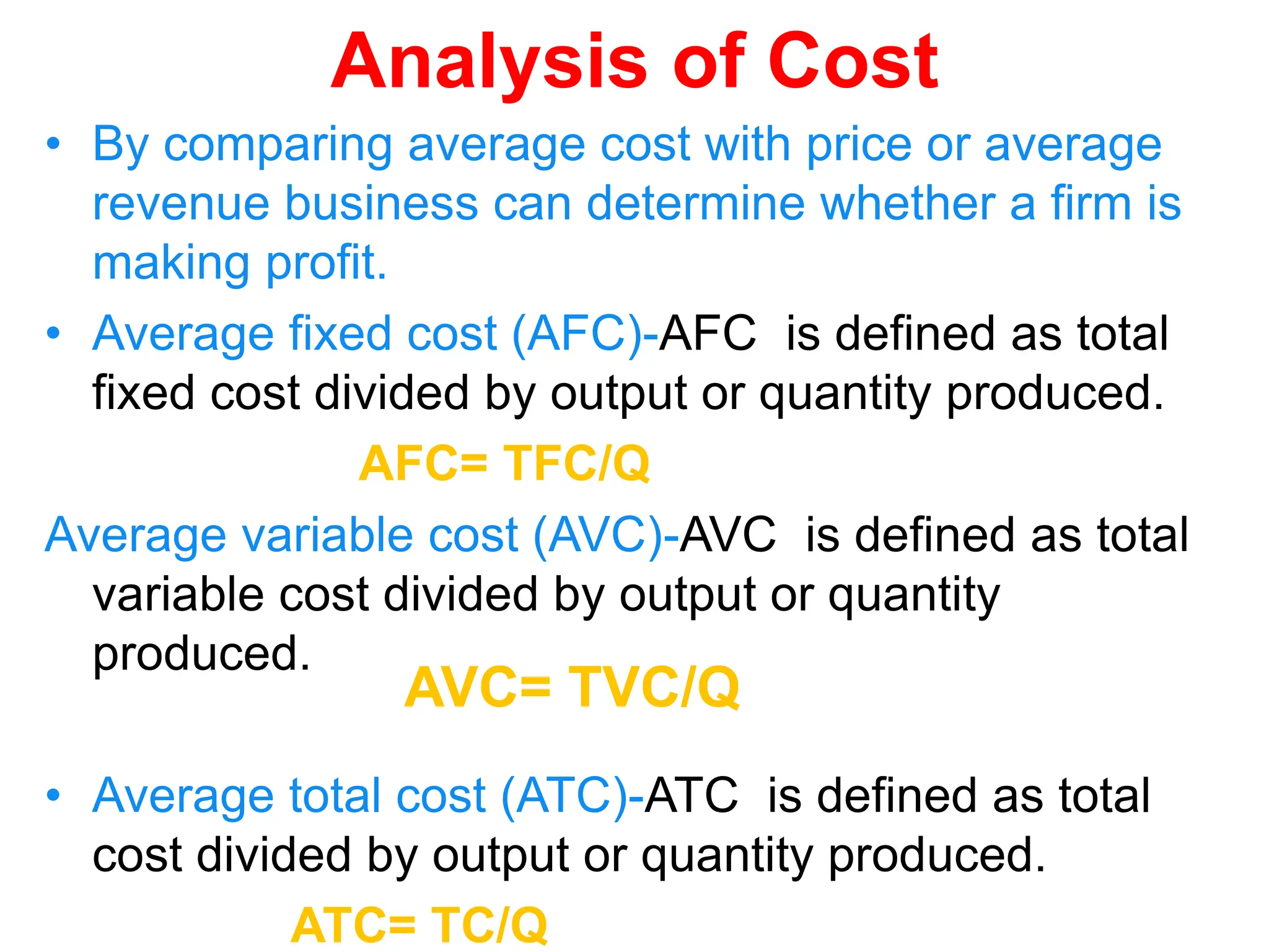
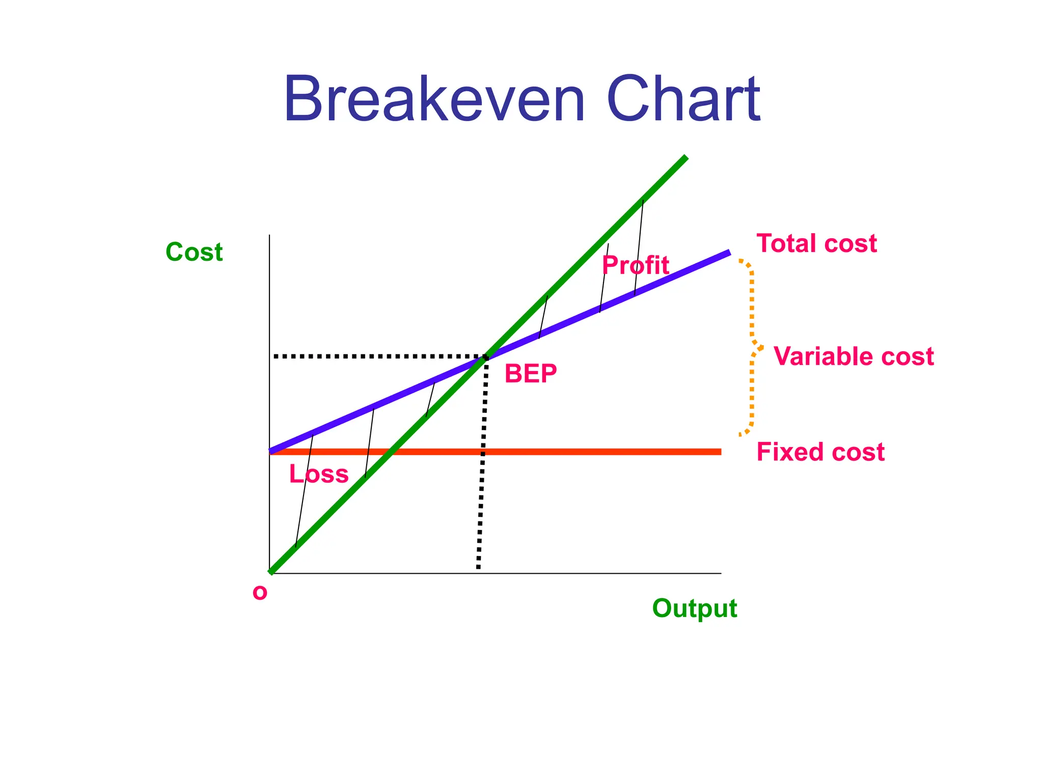
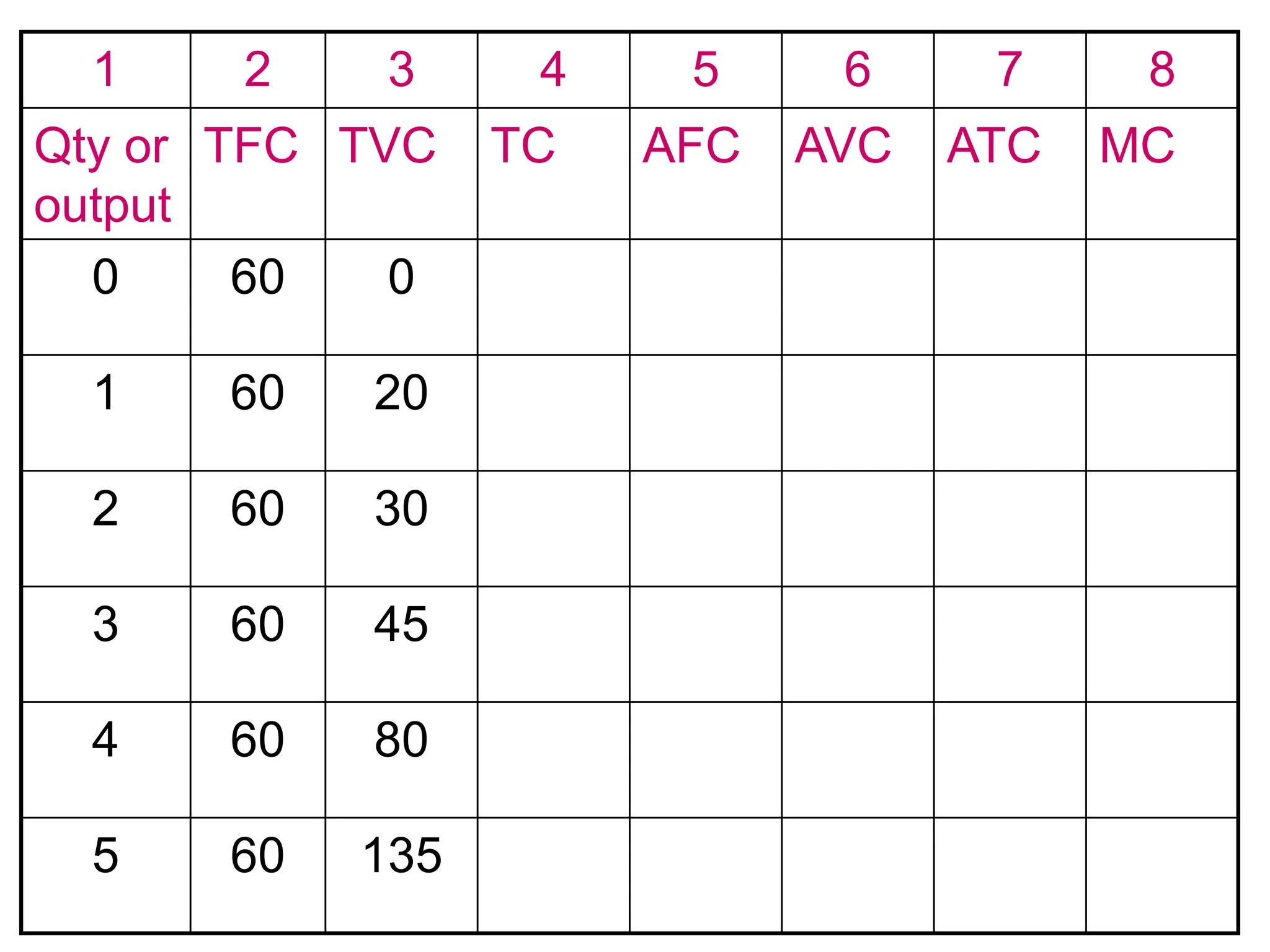
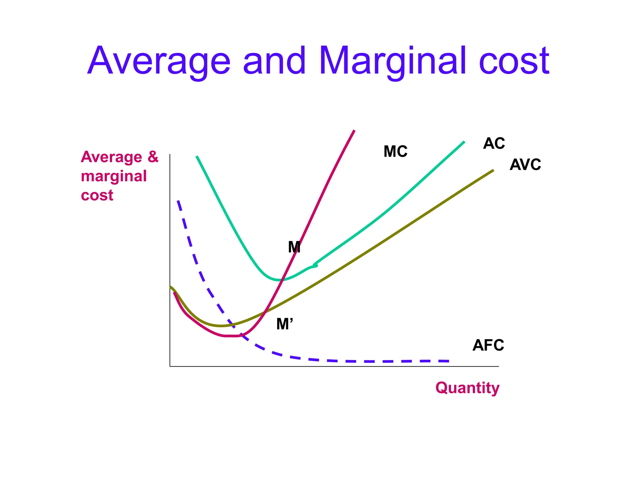
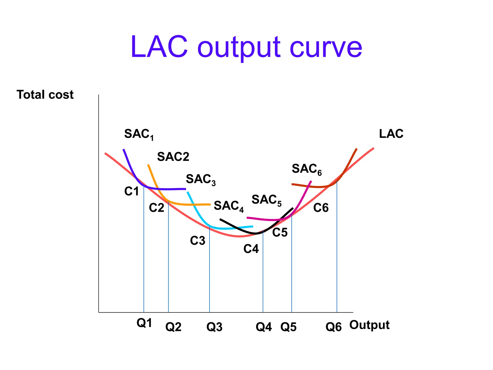
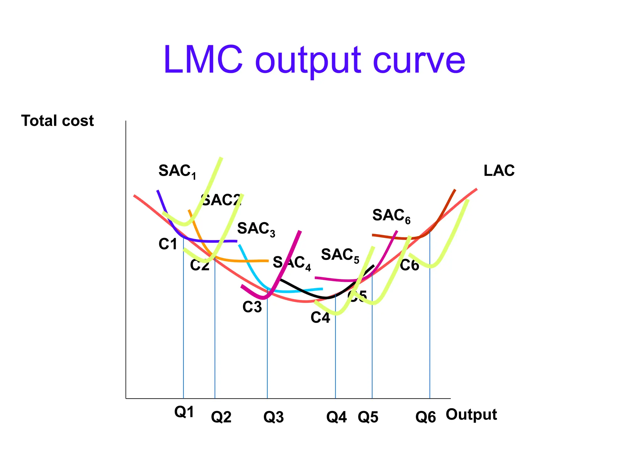
2. Concepts:-
• Production- Production is transformation of
inputs or resources into outputs of goods
and services.
• Inputs-These are the resources used in
production of goods and services. Eg:
Labour, capital , natural resources.

3. Concepts:-
INPUTS
Fixed Variable

4. Concepts:-
• Fixed inputs-The inputs which cannot be
readily changed during the given time period
except when heavy expense is incurred. Eg:
Heavy machinery, Factory, Permanent
workers.
• Variable inputs-The inputs which can be
readily changed during the given time period
at a very short notice. Eg: Contract labour,
Raw material.

5. Concepts:-
• Short Run time period- The time period
during which atleast one input is fixed.
Eg: Production in any industry using more
labour and raw material with old
equipments.
• Long Run time period-The time period when
all inputs are variable. Eg: Increase in
production in any industry using latest
automated equipment.

6. Concepts:-
Production Function: A schedule (or table
or mathematical equation) showing the
maximum amount of output that can be
produced from any specified set of inputs.
Where,
“L” is amount of labour used in production
“K” is capital used in production
In production function we use Labour and capital as
the two inputs
Q= ƒ( L, K)

7. Concepts:
• Variable proportions production-
Production in which a given level of output
can be produced with more than one
combination of inputs.
• Fixed proportions production-Production in
which one, and only one, ratio or mix of
inputs can be used to produce goods.

8. Concepts:
• Technical efficiency: Production of the
maximum level of output that can be
obtained from a given combination of
inputs
• Economic efficiency: Production of a
given amount of output at the lowest
possible cost.

9. Production In The Short Run
Simplest short run situation/ One
variable input
- Only one variable input and one
fixed input.
Q = ƒ( L , )
K
Where,
“Q” is maximum output
“ L” is amount of labour (Variable)
“ K” is level of capital (Investment) fixed

10. Concept of product
• Total product is the total output
produced by a given input when all
other inputs are held constant. As the
input increases out put increases.
In the beginning the total product curve
shows a rise at an increasing rate but as the
variable input is increased further the curve
Starts rising at diminishing rate.

11. Total Products

12. Concept of product
• Average product is the total output
produced per unit of the factor
employed.
Average =
product
Total product
Number of units of a input
employed

13. Marginal product of labour (MP)
The additional output attributable to using
one additional worker with the use of all
other inputs fixed.
Marginal Product= ---------
ΔQ
ΔL

14. Total, Average and marginal products
L Q AP=Q/L MP=ΔQ/ ΔL
1 52 52 52
2 112 56 60
3 170 56.7 58
4 220 55 50
5 258 51.6 38
6 286 47.7 28
7 304 43.4 18
8 314 39.3 10
9 318 35.3 4
10 314 31.4 -4

15. Average and marginal products
Average product
Marginal
product

16. Law of Diminishing Marginal
Product
The principle that as the number of units of the variable
input increases, other inputs held constant, a point will
be reached beyond which the marginal product
decreases.
This law holds true when one gets less output even on
adding additional doses of an input while holding other
inputs fixed. The marginal product of each unit of input
will decline as the amount of that input increases,
holding all other inputs constant

17. Long Run Situation/Production
function with two variable inputs
• Situation in which two inputs are variable.
Production Isoquants-
A curve or locus of points showing all possible
combinations of inputs physically capable of
producing a given fixed level of output.

18. Production function with Two variable inputs
0 1 2 3 4 5 6
3 8 12 14 14 12
7 18 28 30 30 28
10 23 33 36 36 33
12 28 36 40 40 36
12 28 36 40 42 40
10 24 31 36 40 39
LABOUR (L)
CAPITAL(K)
OUTPUT(Q)

19. CAPITAL
LABOUR
12Q
12Q
28Q
28Q
36Q
36Q
40Q
40Q
ISOQUANTS
RIDGE LINES
PRODUCTION ISOQUANTS
V
I
Z

20. PRODUCTION ISOQUANTS
Characteristics-
• The combination of labour and capital can be
changed to get a fixed level of output.
• Two Isoquants never intersect.
• A group of Isoquants is called an Isoquant map.
• All isoquants lying above a given isoquant and to
the right indicate higher levels of output.
• Combinations other than on Isoquants can be
used to produce the given level of output but the
combination will not reflect “ maximum amount of
output” due to the wastage.
• Isoquants are negatively sloped in the
economically relevant range.

21. Marginal rate of technical
substitution (MRTS)
The rate at which one input is substituted for
another along an isoquant.
MRTS = (-) ---------
Δ K
Δ L
If the firm wants to reduce the quantity of capital that
it uses in production, it must increase the quantity
of labour in order to remain on the same isoquant.

22. Shape of Isoquant
LABOUR
CAPITAL
Perfect Substitute Complements inputs
•Smaller the curvature of an isoquant, the greater is the degree of
substitutabilityof inputs in production.
•Greater the curvature of an isoquant the smaller is the degree of
substitutability
LABOUR
CAPITAL

23. Returns to Scale
Returns to scale refers to the degree by
which output changes as a result of a given
change in the quantity of all inputs used in
Production.
Returns to scale are of three types-
1. Increasing returns to scale
2. Decreasing returns to scale
3. Constant returns to scale

24. Returns to Scale
1. Increasing returns to scale- Conditions in
which all inputs are increased by the same
proportion and output increases more than that
proportion.
2. Decreasing returns to scale-Conditions in
which all inputs are increased by the same
proportion and output increases by less than
that proportion.
3. Constant returns to scale-Conditions in
which all inputs are increased by the same
proportion and output increases exactly by
that proportion.

25. Economies of scale
• Economies of scale
• Diseconomies of scale
E=D
E<D
E>D
ATC
Output
E: Economies
D: Diseconomies

26. Economies of scale
Economies of scale: The range of output over
which long run average cost (LAC) falls as output
increases.
When the average cost falls as the plant size
Increases.
Diseconomies of scale :The range of output over
which long run average cost (LAC) rises as output
increases.
When the average cost increases as the plant size
Increases
This occurs in only long run average cost Curve.

27. Economies of scale
Economies of scale: This is of two types-
• External-External economies arise
due to expansion of industry as a
whole. It is a change at macro level.
• Internal-Internal economies arise due
to expansion of firm only.It includes
labour, technology etc.

28. Analysis of Cost
• Fixed cost- Fixed cost are defined as those
which remain the same at a given capacity and
do not vary with output. This cost would exist
even if no output is produced.
• Variable cost- Variable cost are defined as
those which vary directly as output changes
This cost would not exist if no output is
produced.
• Total cost-Total cost is the sum of fixed cost
and variable cost.
TC= TFC+TVC

29. Analysis of Cost
• By comparing average cost with price or average
revenue business can determine whether a firm is
making profit.
• Average fixed cost (AFC)-AFC is defined as total
fixed cost divided by output or quantity produced.
AFC= TFC/Q
Average variable cost (AVC)-AVC is defined as total
variable cost divided by output or quantity
produced.
• Average total cost (ATC)-ATC is defined as total
cost divided by output or quantity produced.
ATC= TC/Q
AVC= TVC/Q

30. Breakeven Chart
o
Fixed cost
Total cost
Variable cost
BEP
Loss
Profit
Output
Cost

31. 1 2 3 4 5 6 7 8
Qty or
output
TFC TVC TC AFC AVC ATC MC
0 60 0
1 60 20
2 60 30
3 60 45
4 60 80
5 60 135

32. Average and Marginal cost
MC
AC
AVC
AFC
Quantity
Average &
marginal
cost
M’
M

33. Cost Curve
• When marginal cost is below average cost, it is
pulling average cost down.
• When marginal cost is above average cost, it is
pulling average cost up
• When marginal cost is equal to average cost,
average cost is neither rising nor falling and it is
at its minimum. Hence at the bottom of u shaped
AC , MC =AC
• The inference is for lowest average cost of
production level of output should be such where
MC=AC

34. Long Run Cost relationships
• In the long run all inputs are variable.
• The firms long run total cost curve is
derived from the firm’s expansion firm i.e.
by combining short run average cost curve
and shows the minimum long run total cost
of producing various levels of output.

35. Total cost output curve
Output
Total cost
LTC
STC3
STC2
STC1
Q1 Q2 Q3

36. Characteristics of LTC,LAC,LMC
• LTC –Long run total cost curve, when the firm
decides to add two or more plants i.e.
STC1,STC2,STC3…………..The LTC can be
drawn through the minimum points of STC1
,STC2,STC3……………
• LAC- Long run average cost curve, LAC is
derived from combination of short run average
cost curves(SAC) as we add on more plants the
SAC becomes lesser. From the mid points of all
SACs the LAC can be derived . The LAC is also
known as envelop curve or planning curve.

37. LAC output curve
Output
Total cost
LAC
SAC3
SAC1
Q1 Q2 Q3
SAC2
SAC4
SAC5
SAC6
Q4 Q6
Q5
C1
C2
C3
C4
C5
C6

38. LMC output curve
Output
Total cost
LAC
SAC3
SAC1
Q1 Q2 Q3
SAC2
SAC4
SAC5
SAC6
Q4 Q6
Q5
C1
C2
C3
C4
C5
C6