The document discusses sampled functions and their z-transforms. It begins by explaining how sampling a continuous function at intervals of T produces a sequence of values. The z-transform of this sampled sequence is then related to the Laplace transform of the original continuous function. Specifically, the z-transform of the sampled sequence is equivalent to the Laplace transform with s replaced by z=esT. Examples are provided to illustrate this relationship between the pole locations of the two transforms.

1. Sampled Functions
21.5
Introduction
A sequence can be obtained by sampling a continuous function or signal and in this Section we
show first of all how to extend our knowledge of z-transforms so as to be able to deal with sampled
signals. We then show how the z-transform of a sampled signal is related to the Laplace transform
of the unsampled version of the signal.
'
$
%
Prerequisites
Before starting this Section you should . . .
• possess an outline knowledge of Laplace
transforms and of z-transforms
9
8
6
7
Learning Outcomes
On completion you should be able to . . .
• take the z-transform of a sequence obtained
by sampling
• state the relation between the z-transform of
a sequence obtained by sampling and the
Laplace transform of the underlying
continuous signal
HELM (2005):
Section 21.5: Sampled Functions
85

2. 1. Sampling theory
If a continuous-time signal f(t) is sampled at terms t = 0, T, 2T, . . . nT, . . . then a sequence of
values
{f(0), f(T), f(2T), . . . f(nT), . . .}
is obtained. The quantity T is called the sample interval or sample period.
t
T 2T nT
f(t)
Figure 18
In the previous Sections of this Workbook we have used the simpler notation {fn} to denote a
sequence. If the sequence has actually arisen by sampling then fn is just a convenient notation for
the sample value f(nT).
Most of our previous results for z-transforms of sequences hold with only minor changes for sampled
signals.
So consider a continuous signal f(t); its z-transform is the z-transform of the sequence of sample
values i.e.
Z{f(t)} = Z{f(nT)} =
∞
n=0
f(nT)z−n
We shall briefly obtain z-transforms of common sampled signals utilizing results obtained earlier. You
may assume that all signals are sampled at 0, T, 2T, . . . nT, . . .
Unit step function
u(t) =
1 t ≥ 0
0 t 0
Since the sampled values here are a sequence of 1’s,
Z{u(t)} = Z{un} =
1
1 − z−1
=
z
z − 1
|z| 1
where {un} = {1, 1, 1, . . .} is the unit step sequence.
↑
86 HELM (2005):
Workbook 21: z-Transforms

3. Ramp function
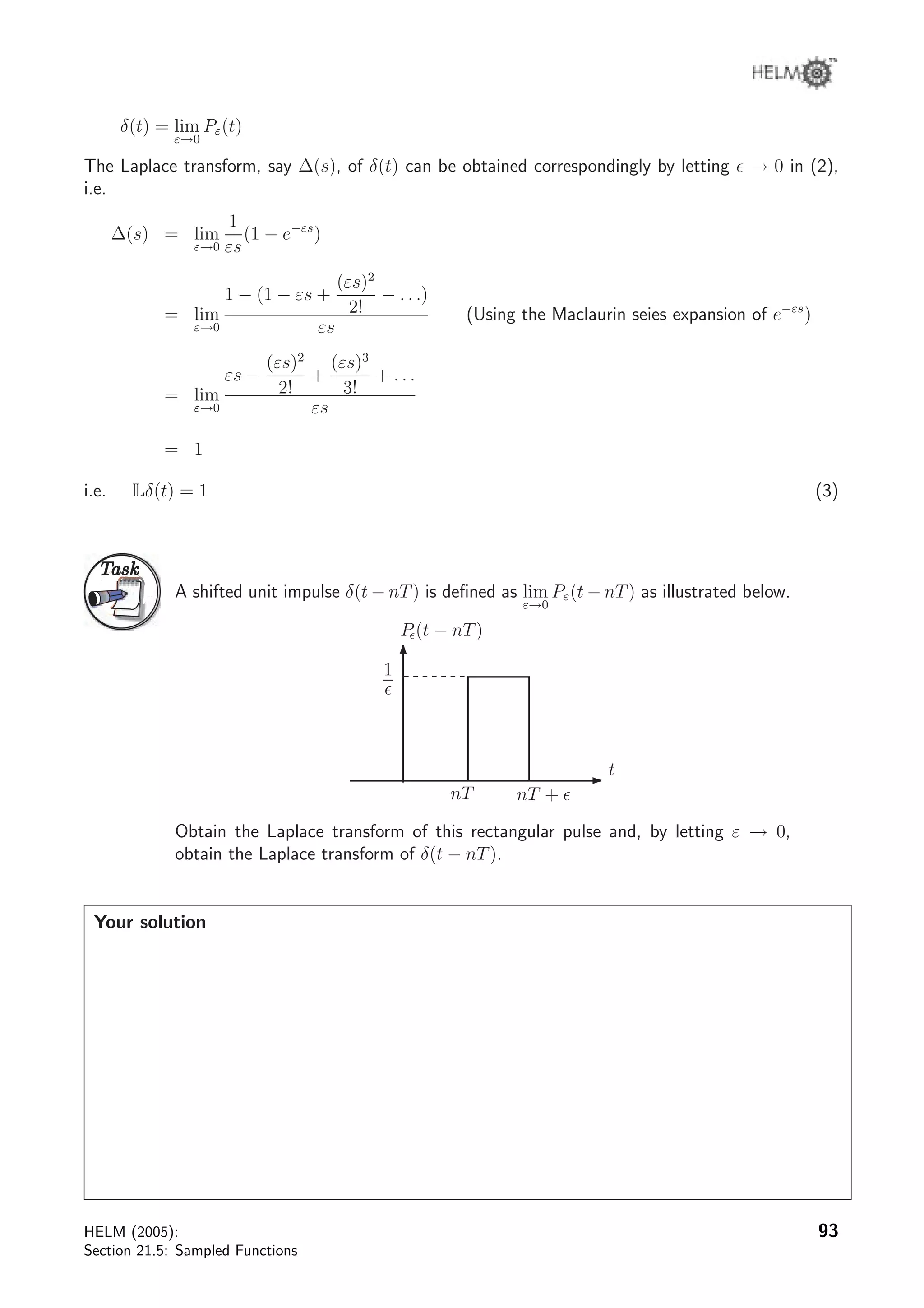
r(t) =
t t ≥ 0
0 t 0
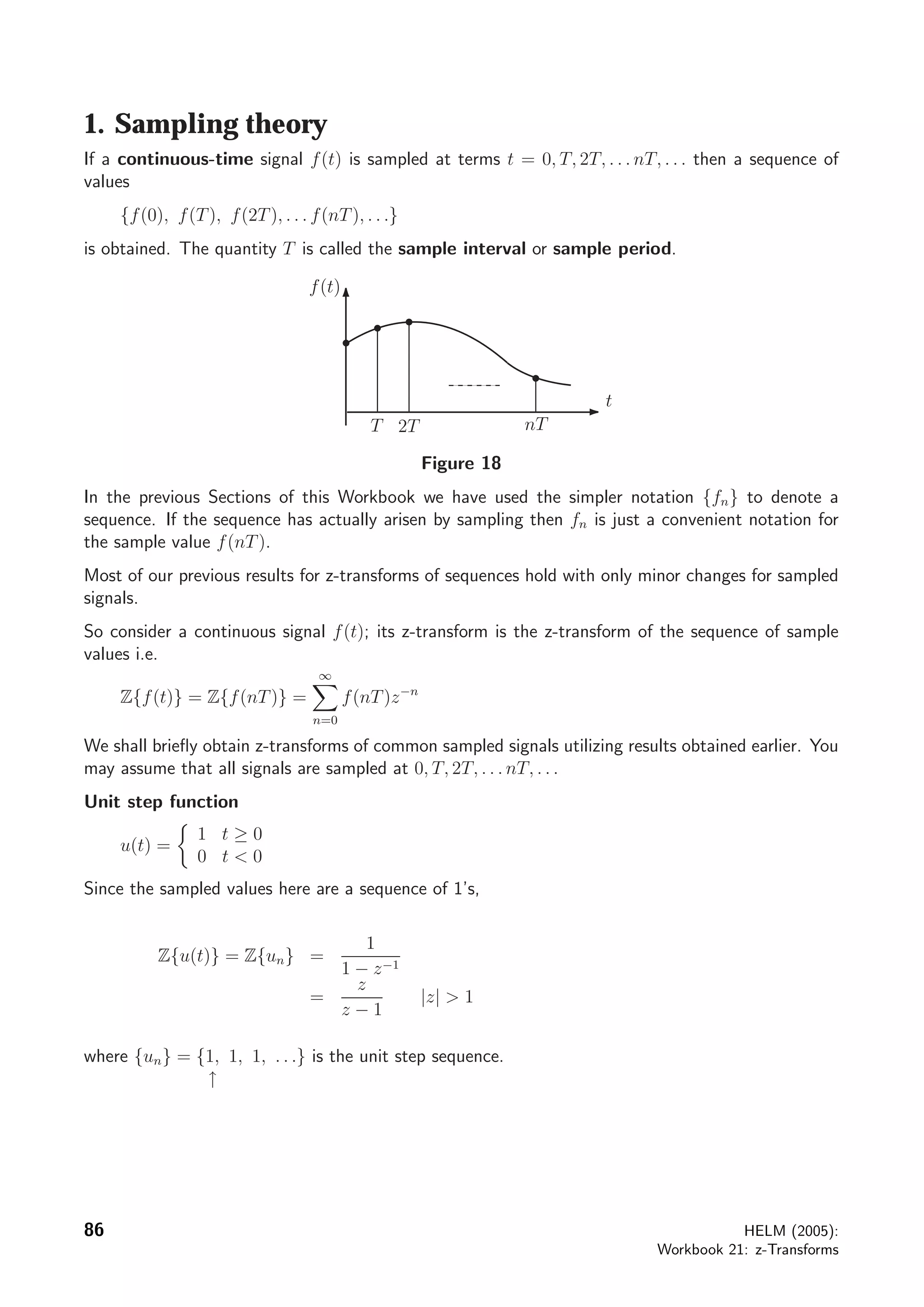
The sample values here are
{r(nT)} = {0, T, 2T, . . .}
The ramp sequence {rn} = {0, 1, 2, . . .} has z-transform
z
(z − 1)2
.
Hence Z{r(nT)} =
Tz
(z − 1)2
since {r(nT)} = T{rn}.
TaskTask
Obtain the z-transform of the exponential signal
f(t) =
e−αt
t ≥ 0
0 t 0.
[Hint: use the z-transform of the geometric sequence {an
}.]
Your solution
Answer
The sample values of the exponential are
{1, e−αT
, e−α2T
, . . . , e−αnT
, . . .}
i.e. f(nT) = e−αnT
= (e−αT
)n
.
But Z{an
} =
z
z − a
∴ Z{(e−αT
)n
} =
z
z − e−αT
=
1
1 − e−αT z−1
HELM (2005):
Section 21.5: Sampled Functions
87

4. Sampled sinusoids
Earlier in this Workbook we obtained the z-transform of the sequence {cos ωn} i.e.
Z{cos ωn} =
z2
− z cos ω
z2 − 2z cos ω + 1
Hence, since sampling the continuous sinusoid
f(t) = cos ωt
yields the sequence {cos nωT} we have, simply replacing ω by ωT in the z-transform:
Z{cos ωt} = Z{cos nωT}
=
z2
− z cos ωT
z2 − 2z cos ωT + 1
TaskTask
Obtain the z-transform of the sampled version of the sine wave f(t) = sin ωt.
Your solution
Answer
Z{sin ωn} =
z sin ω
z2 − 2z cos ω + 1
∴ Z{sin ωt} = Z{sin nωT}
=
z sin ωT
z2 − 2z cos ωT + 1
88 HELM (2005):
Workbook 21: z-Transforms

5. Shift theorems
These are similar to those discussed earlier in this Workbook but for sampled signals the shifts are
by integer multiples of the sample period T. For example a simple right shift, or delay, of a sampled
signal by one sample period is shown in the following figure:
t
T 2T
t
T 2T
3T
3T
f(nT)
f(nT − T)
4T
Figure 19
The right shift properties of z-transforms can be written down immediately. (Look back at the shift
properties in Section 21.2 subsection 5, if necessary:)
If y(t) has z-transform Y (z) which, as we have seen, really means that its sample values {y(nT)}
give Y (z), then for y(t) shifted to the right by one sample interval the z-transform becomes
Z{y(t − T)} = y(−T) + z−1
Y (z)
The proof is very similar to that used for sequences earlier which gave the result:
Z{yn−1} = y−1 + z−1
Y (z)
TaskTask
Using the result
Z{yn−2} = y−2 + y−1z−1
+ z−2
Y (z)
write down the result for Z{y(t − 2T)}
Your solution
Answer
Z{y(t − 2T)} = y(−2T) + y(−T)z−1
+ z−2
Y (z)
These results can of course be generalised to obtain Z{y(t − mT)} where m is any positive integer.
In particular, for causal or one-sided signals y(t) (i.e. signals which are zero for t 0):
Z{y(t − mT)} = z−m
Y (z)
Note carefully here that the power of z is still z−m
not z−mT
.
HELM (2005):
Section 21.5: Sampled Functions
89

6. Examples:
For the unit step function we saw that:
Z{u(t)} =
z
z − 1
=
1
1 − z−1
Hence from the shift properties above we have immediately, since u(t) is certainly causal,
Z{u(t − T)} =
zz−1
z − 1
=
z−1
1 − z−1
Z{u(t − 3T)} =
zz−3
z − 1
=
z−3
1 − z−1
and so on.
t
T 2T
t
T 2T
3T
3T 5T4T
u(t − T)
u(t − 3T)
Figure 20
2. z-transforms and Laplace transforms
In this Workbook we have developed the theory and some applications of the z-transform from first
principles. We mentioned much earlier that the z-transform plays essentially the same role for discrete
systems that the Laplace transform does for continuous systems. We now explore the precise link
between these two transforms. A brief knowledge of Laplace transform will be assumed.
At first sight it is not obvious that there is a connection. The z-transform is a summation defined,
for a sampled signal fn ≡ f(nT), as
F(z) =
∞
n=0
f(nT)z−n
while the Laplace transform written symbolically as L{f(t)} is an integral, defined for a continuous
time function f(t), t ≥ 0 as
F(s) =
∞
0
f(t)e−st
dt.
90 HELM (2005):
Workbook 21: z-Transforms

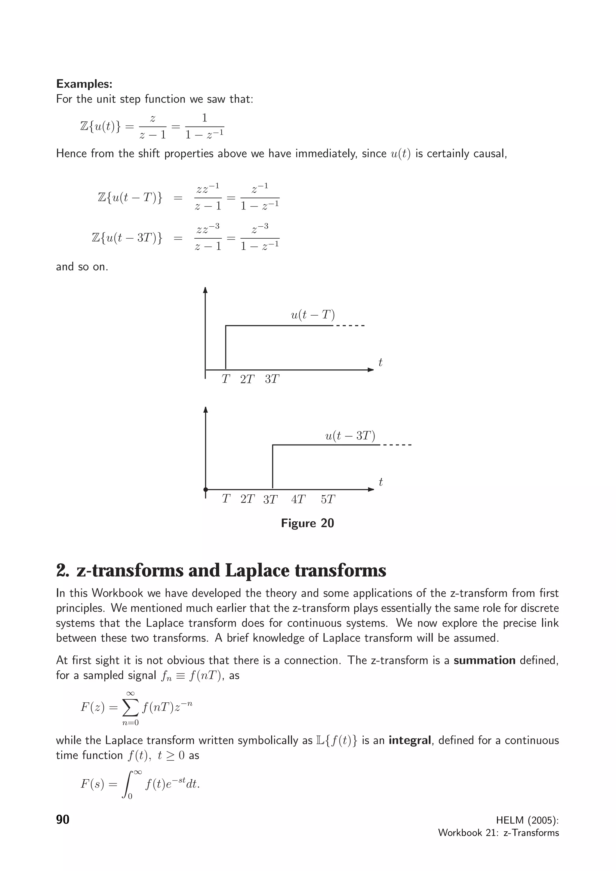
7. Thus, for example, if
f(t) = e−αt
(continuous time exponential)
L{f(t)} = F(s) =
1
s + α
which has a (simple) pole at s = −α = s1 say.
As we have seen, sampling f(t) gives the sequence {f(nT)} = {e−αnT
} with z-transform
F(z) =
1
1 − e−αT z−1
=
z
z − e−αT
.
The z-transform has a pole when z = z1 where
z1 = e−αT
= es1T
[Note the abuse of notations in writing both F(s) and F(z) here since in fact these are different
functions.]
TaskTask
The continuous time function f(t) = te−αt
has Laplace transform
F(s) =
1
(s + α)2
Firstly write down the pole of this function and its order:
Your solution
Answer
F(s) =
1
(s + α)2
has its pole at s = s1 = −α. The pole is second order.
Now obtain the z-transform F(z) of the sampled version of f(t), locate the pole(s) of F(z) and
state the order:
Your solution
HELM (2005):
Section 21.5: Sampled Functions
91

8. Answer
Consider f(nT) = nTe−αnT
= (nT)(e−αT
)n
The ramp sequence {nT} has z-transform
Tz
(z − 1)2
∴ f(nT) has z-transform
F(z) =
TzeαT
(zeαT − 1)2
=
Tze−αT
(z − e−αT )2
(see Key Point 8)
This has a (second order) pole when z = z1 = e−αT
= es1T
.
We have seen in both the above examples a close link between the pole s1 of the Laplace transform
of f(t) and the pole z1 of the z-transform of the sampled version of f(t) i.e.
z1 = es1T
(1)
where T is the sample interval.
Multiple poles lead to similar results i.e. if F(s) has poles s1, s2, . . . then F(z) has poles z1, z2, . . .
where zi = esiT
.
The relation (1) between the poles is, in fact, an example of a more general relation between the
values of s and z as we shall now investigate.
Key Point 19
The unit impulse function δ(t) can be defined informally as follows:
t
1
P (t)
Figure 21
The rectangular pulse P (t) of width ε and height
1
ε
shown in Figure 21 encloses unit area and has
Laplace transform
Pε(s) =
ε
0
1
ε
e−st
=
1
εs
(1 − e−εs
) (2)
As ε becomes smaller Pε(t) becomes taller and narrower but still encloses unit area. The unit impulse
function δ(t) (sometimes called the Dirac delta function) can be defined as
92 HELM (2005):
Workbook 21: z-Transforms

9. δ(t) = lim
ε→0
Pε(t)
The Laplace transform, say ∆(s), of δ(t) can be obtained correspondingly by letting → 0 in (2),
i.e.
∆(s) = lim
ε→0
1
εs
(1 − e−εs
)
= lim
ε→0
1 − (1 − εs +
(εs)2
2!
− . . .)
εs
(Using the Maclaurin seies expansion of e−εs
)
= lim
ε→0
εs −
(εs)2
2!
+
(εs)3
3!
+ . . .
εs
= 1
i.e. Lδ(t) = 1 (3)
TaskTask
A shifted unit impulse δ(t − nT) is defined as lim
ε→0
Pε(t − nT) as illustrated below.
t
1
nT nT +
P (t − nT)
Obtain the Laplace transform of this rectangular pulse and, by letting ε → 0,
obtain the Laplace transform of δ(t − nT).
Your solution
HELM (2005):
Section 21.5: Sampled Functions
93

10. Answer
L{Pε(t − nT)} =
nT+ε
nT
1
ε
e−st
dt =
1
εs
− e−st
nT+ε
nT
=
1
εs
e−snT
− e−s(nT+ε)
=
1
εs
e−snT
(1 − e−sε
) → e−snT
as ε → 0
Hence L{δ(t − nT)} = e−snT
(4)
which reduces to the result (3)
L{δ(t)} = 1 when n = 0
These results (3) and (4) can be compared with the results
Z{δn} = 1
Z{δn−m} = z−m
for discrete impulses of height 1.
Now consider a continuous function f(t). Suppose, as usual, that this function is sampled at t = nT
for n = 0, 1, 2, . . .
t
T 2T
f(t)
4T3T
Figure 22
This sampled equivalent of f(t), say f∗(t) can be defined as a sequence of equidistant impulses, the
‘strength’ of each impulse being the sample value f(nT)i.e.
f∗(t) =
∞
n=0
f(nT)δ(t − nT)
This function is a continuous-time signal i.e. is defined for all t. Using (4) it has a Laplace transform
F∗(s) =
∞
n=0
f(nT)e−snT
(5)
If, in this sum (5) we replace esT
by z we obtain the z-transform of the sequence {f(nT)} of samples:
∞
n=0
f(nT)z−n
94 HELM (2005):
Workbook 21: z-Transforms

11. Key Point 20
The Laplace transform
F(s) =
∞
n=0
f(nT)e−snT
of a sampled function is equivalent to the z-transform F(z) of the sequence {f(nT)} of sample
values with z = esT
.
Table 2: z-transforms of some sampled signals
This table can be compared with the table of the z-transforms of sequences on the following page.
f(t) f(nT) F(z) Radius of convergence
t ≥ 0 n = 0, 1, 2, . . . R
1 1
z
z − 1
1
t nT
z
(z − 1)2
1
t2
(nT)2 T2
z(z + 1)
(z − 1)3
1
e−αt
e−αnT z
z − e−αT
|e−αT
|
sin ωt sin nωT
z sin ωT
z2 − 2z cos ωT + 1
1
cos ωt cos nωT
z(z − cos ωT)
z2 − 2z cos ωT + 1
1
te−αt
nTe−αnT Tze−αT
(z − e−αT )2
|e−αT
|
e−αt
sin ωt e−αnT
sin ωnT
e−αT
z−1
sin ωT
1 − 2e−αT z−1 cos ωT + e−2aT z−2
|e−αT
|
e−αT
cos ωt e−αnT
cos ωnT
1 − e−αT
z−1
cos ωT
1 − 2e−αT z−1 cos ωT + e−2aT z−2
|e−αT
|
Note: R is such that the closed forms of F(z) (those listed in the above table) are valid for |z| R.
HELM (2005):
Section 21.5: Sampled Functions
95

12. Table of z-transforms
fn F(z) Name
δn 1 unit impulse
δn−m z−m
un
z
z − 1
unit step sequence
an z
z − a
geometric sequence
eαn z
z − eα
sinh αn
z sinh α
z2 − 2z cosh α + 1
cosh αn
z2
− z cosh α
z2 − 2z cosh α + 1
sin ωn
z sin ω
z2 − 2z cos ω + 1
cos ωn
z2
− z cos ω
z2 − 2z cos ω + 1
e−αn
sin ωn
ze−α
sin ω
z2 − 2ze−α cos ω + e−2α
e−αn
cos ωn
z2
− ze−α
cos ω
z2 − 2ze−α cos ω + e−2α
n
z
(z − 1)2
ramp sequence
n2 z(z + 1)
(z − 1)3
n3 z(z2
+ 4z + 1)
(z − 1)4
an
fn F
z
a
n fn −z
dF
dz
96 HELM (2005):
Workbook 21: z-Transforms