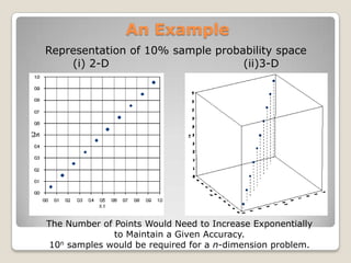
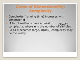
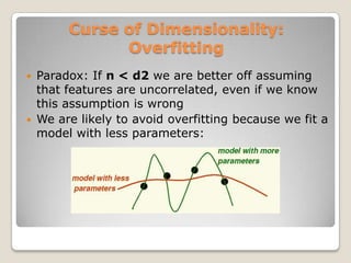
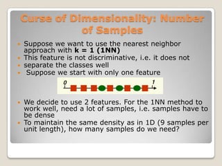
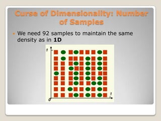
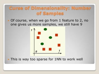
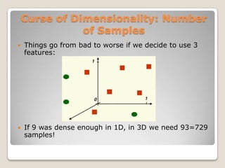
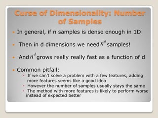
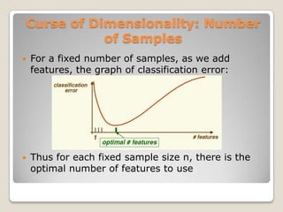
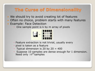
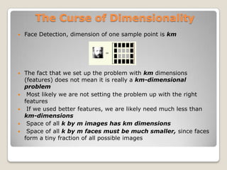
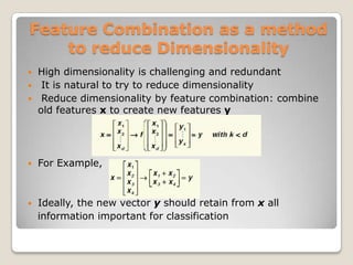
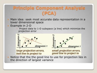
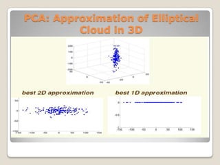
The document discusses the curse of dimensionality, which refers to the problem caused by an exponential increase in volume associated with adding extra dimensions to a mathematical space. This causes several issues, including an increase in running time and overfitting as the number of dimensions increases. It also requires exponentially more samples to maintain the same level of accuracy as more dimensions are added. Several methods are discussed to help address this problem, such as dimensionality reduction techniques like principal component analysis, which projects the data onto a lower dimensional space.
2. What is it?
In applied mathematics, curse of
dimensionality (a term coined by Richard E.
Bellman), also known as the Hughes
effect (named after Gordon F. Hughes),refers to
the problem caused by the exponential increase
in volume associated with adding extra
dimensions to a mathematical space.
3. Problems
• High Dimensional Data is difficult to work with
since:
Adding more features can increase the noise, and
hence the error
There usually aren’t enough observations to get
good estimates
• This causes:
Increase in running time
Overfitting
Number of Samples Required
4. An Example
Representation of 10% sample probability space
(i) 2-D (ii)3-D
The Number of Points Would Need to Increase Exponentially
to Maintain a Given Accuracy.
10n samples would be required for a n-dimension problem.
5. Curse of Dimensionality:
Complexity
Complexity (running time) increases with
dimension d
A lot of methods have at least
O(nd 2 )
complexity, where n is the number of samples
So as d becomes large, O(nd2) complexity may
be too costly
6. Curse of Dimensionality:
Overfitting
Paradox: If n < d2 we are better off assuming
that features are uncorrelated, even if we know
this assumption is wrong
We are likely to avoid overfitting because we fit a
model with less parameters:
7. Curse of Dimensionality: Number
of Samples
Suppose we want to use the nearest neighbor
approach with k = 1 (1NN)
This feature is not discriminative, i.e. it does not
separate the classes well
Suppose we start with only one feature
We decide to use 2 features. For the 1NN method to
work well, need a lot of samples, i.e. samples have to
be dense
To maintain the same density as in 1D (9 samples per
unit length), how many samples do we need?
8. Curse of Dimensionality: Number
of Samples
We need 92 samples to maintain the same
density as in 1D
9. Curse of Dimensionality: Number
of Samples
Of course, when we go from 1 feature to 2, no
one gives us more samples, we still have 9
This is way too sparse for 1NN to work well
10. Curse of Dimensionality: Number
of Samples
Things go from bad to worse if we decide to use 3
features:
If 9 was dense enough in 1D, in 3D we need 93=729
samples!
11. Curse of Dimensionality: Number
of Samples
In general, if n samples is dense enough in 1D
Then in d dimensions we need n d samples!
And n d grows really really fast as a function of d
Common pitfall:
If we can’t solve a problem with a few features, adding
more features seems like a good idea
However the number of samples usually stays the same
The method with more features is likely to perform worse
instead of expected better
12. Curse of Dimensionality: Number
of Samples
For a fixed number of samples, as we add
features, the graph of classification error:
Thus for each fixed sample size n, there is the
optimal number of features to use
13. The Curse of Dimensionality
We should try to avoid creating lot of features
Often no choice, problem starts with many features
Example: Face Detection
One sample point is k by m array of pixels
Feature extraction is not trivial, usually every
pixel is taken as a feature
Typical dimension is 20 by 20 = 400
Suppose 10 samples are dense enough for 1 dimension.
Need only 10400samples
14. The Curse of Dimensionality
Face Detection, dimension of one sample point is km
The fact that we set up the problem with km dimensions
(features) does not mean it is really a km-dimensional
problem
Most likely we are not setting the problem up with the right
features
If we used better features, we are likely need much less than
km-dimensions
Space of all k by m images has km dimensions
Space of all k by m faces must be much smaller, since faces
form a tiny fraction of all possible images
15. Dimensionality Reduction
We want to reduce the number of
dimensions because:
Efficiency.
Measurement costs.
Storage costs.
Computation costs.
Classification performance.
Ease of interpretation/modeling.
16. Principal Components
The idea is to project onto the subspace which accounts for
most of the variance.
This is accomplished by projecting onto the eigenvectors of
the covariance matrix associated with the largest
eigenvalues.
This is generally not the projection best suited for
classification.
It can be a useful method for providing a first-cut reduction
in dimension from a high dimensional space
17. Feature Combination as a method
to reduce Dimensionality
High dimensionality is challenging and redundant
It is natural to try to reduce dimensionality
Reduce dimensionality by feature combination: combine
old features x to create new features y
For Example,
Ideally, the new vector y should retain from x all
information important for classification
18. Principle Component Analysis
(PCA)
Main idea: seek most accurate data representation in a
lower dimensional space
Example in 2-D
◦ Project data to 1-D subspace (a line) which minimize the
projection error
Notice that the the good line to use for projection lies in
the direction of largest variance
Let's say you have a straight line 100 yards long and you dropped a penny somewhere on it. It wouldn't be too hard to find. You walk along the line and it takes two minutes.Now let's say you have a square 100 yards across and you dropped a penny somewhere on it. It would be pretty hard, like searching across two football fields stuck together. It could take days.Now a cube 100 yards across. That's like searching a 30-story building the size of a football stadium. Ugh.The difficulty of searching through the space gets a *lot* harder as you have more dimensions. You might not realize this intuitively when it's just stated in mathematical formulas, since they all have the same "width". That's the curse of dimensionality. It gets to have a name because it is unintuitive, useful, and yet simple.
Let the complete probability space for one variable be represented by the unit interval (0, 1), and imagine drawing ten samples along that interval. Each sample would then have to represent 10% of the probability space (on average). Now consider a second variable defined on another, orthogonal, (0, 1) interval, also being represented by ten samples. We have produced 10 (x1 , x2 ) points on a plane defined by the orthogonal x1 , x2 lines, and representing a new probability space. But the new space has 10 ? 10 = 100 area units, so each of the ten points now represents only 1% of the probability space. It would require 100 points for each point to represent the same 10% of the probability space that was represented by 10 points in only one dimension. This is illustrated below, where the 10 points are not drawn at random to illustrate their diminished coverage.The Number of Points Would Need to Increase Exponentially to Maintain a Given Accuracy.Now, although there are 100 (x1 , x2 ) points, neither axis has more accuracy than was provided by the previous 10, because there are 10 values of x1 required for the 10 different values of x2 necessary to represent the new probability plane. Because in practice the samples are taken at random it appears as though there are more samples, but this isn't the case in terms of probability space coverage which is related to the density of points, not the number of observations per axis.Next consider adding another dimension creating a probability space represented by a cube with ten units on a side, and 1000 probability units within. It now requires stacking 10 of the previous (x1 , x2 ) planes to construct the new (x1 , x2 , x3 ) cube, and of course 10 times the number of samples per axis to maintain the former level of accuracy, or probability coverage. It is obvious that10n samples would be required for a n-dimension problem.