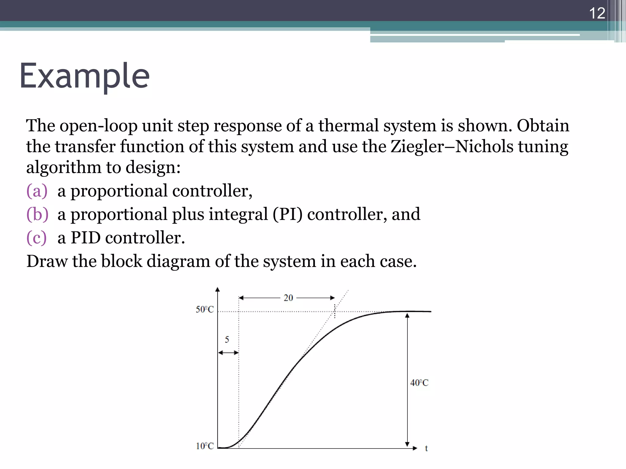
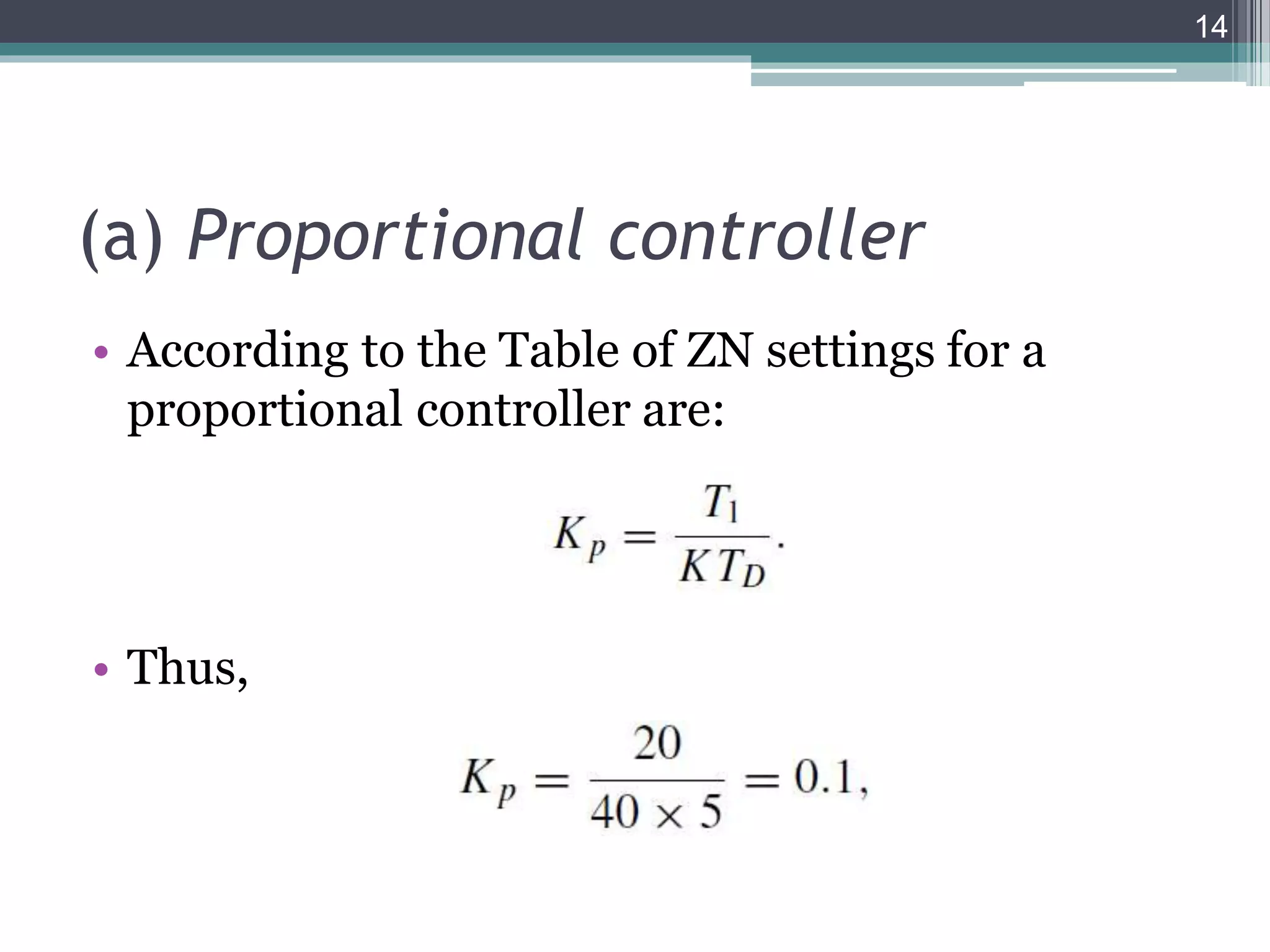
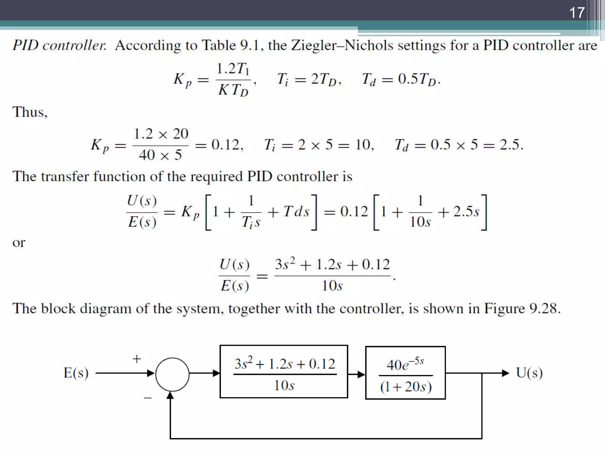
Chapter 9:
Discrete Controller Design
(PID Controller)
1
9.2 PID CONTROLLER
• The proportional–integral–derivative (PID)
controller is often referred to as a ‘three-term’
controller.
• It is one of the most frequently used controllers in
the process industry.
• In a PID controller the control variable is generated
from the sum of a term proportional to the error, a
term which is the integral of the error, and a term
which is the derivative of the error.
2
9.2 PID CONTROLLER
• Proportional: the error is multiplied by a gain Kp. A
very high gain may cause instability, and a very low gain
may cause the system to be very sluggish (slow).
• Integral: the integral of the error is found and
multiplied by a gain. The gain can be adjusted to drive
the error to zero in the required time.
• Derivative: The derivative of the error is multiplied by
a gain. The derivative control is used to improve the
transient response by reducing overshoot.
3
• The input–output relationship of a PID controller can be
expressed as
• where u(t) is the output from the controller and e(t) = r (t) −
y(t), in which r (t) is the desired set-point (reference input)
and y(t) is the plant output. Ti and Td are known as the
integral and derivative action time, respectively.
• By taking the Laplace transform of this equation, we can write
the transfer function of a continuous-time PID as
4
5
• To implement the PID controller using a digital computer we have
to convert the equation:
from a continuous to a discrete representation.
• There are several methods for doing this and the simplest is to use
the trapezoidal approximation for the integral and the backward
difference approximation for the derivative:
6
Discrete PID Controller
0
𝑡
𝑒 𝑡 𝑑𝑡 ≈ 𝑘=1
𝑛
𝑇𝑒 𝑘𝑇 ,
𝑑𝑒(𝑡)
𝑑𝑡
≈
𝑒 𝑛𝑇 −𝑒(𝑛𝑇−𝑇)
𝑇
• Using these approximations, we can write:
𝑢 𝑛𝑇 = 𝐾𝑝[𝑒 𝑛𝑇 +
1
𝑇𝑖
𝑘=1
𝑛
𝑇𝑒 𝑘𝑇 + 𝑇𝑑
𝑒 𝑛𝑇 −𝑒(𝑛𝑇−𝑇)
𝑇
],
𝑢 𝑛𝑇 − 𝑇 = 𝐾𝑝[𝑒 𝑛𝑇 − 𝑇 +
1
𝑇𝑖
𝑘=1
𝑛−1
𝑇𝑒 𝑘𝑇 + 𝑇𝑑
𝑒 𝑛𝑇−𝑇 −𝑒(𝑛𝑇−2𝑇)
𝑇
].
• Subtracting these two equations, we obtain:
𝑢𝑛 = 𝑢𝑛−1 + 𝐾𝑝 𝑒𝑛 − 𝑒𝑛−1 +
𝐾𝑝𝑇
𝑇𝑖
𝑒𝑛 +
𝐾𝑝𝑇𝑑
𝑇
[𝑒𝑛 − 2𝑒𝑛−1 + 𝑒𝑛−2]
where 𝑢𝑛: = 𝑢(𝑛𝑇) and 𝑢𝑛−1: = 𝑢 𝑛𝑇 − 𝑇 .
• The PID is now in a suitable form which can be implemented on a digital
computer. Here the current control action uses the previous control value
as a reference.
7
9.2.3 PID Tuning
• Tuning the controller involves adjusting the
parameters Kp, Td and Ti in order to obtain a
satisfactory response.
• There are many techniques for tuning a controller,
ranging from the first techniques described by J.G.
Ziegler and N.B. Nichols (known as the Ziegler–
Nichols tuning algorithm), to recent auto-tuning
controllers.
• In this section we shall look at the tuning of PID
controllers using the Ziegler–Nichols tuning
algorithm.
8
• Ziegler and Nichols suggested values for the PID
parameters of a plant based on open-loop or closed-
loop tests of the plant.
• According to Ziegler and Nichols, the open-loop
transfer function of a system can be approximated
with a time delay and a single-order system, i.e.
• where TD is the system time delay (i.e.
transportation delay), and T1 is the time constant of
the system.
9
• For open-loop tuning, we first find the plant parameters by applying
a step input to the open loop system.
• The plant parameters K, TD and T1 are then found from the result of
the step test as shown.
10
• Ziegler and Nichols then suggest using the PID controller settings
given in the Table below when the loop is closed.
• These parameters are based on the concept of minimizing the
integral of the absolute error after applying a step change to the set-
point.
11
Example
The open-loop unit step response of a thermal system is shown. Obtain
the transfer function of this system and use the Ziegler–Nichols tuning
algorithm to design:
(a) a proportional controller,
(b) a proportional plus integral (PI) controller, and
(c) a PID controller.
Draw the block diagram of the system in each case.
12
Solution
• From the previous Figure, the system
parameters are obtained as K = 40◦C, TD = 5 s
and T1 = 20 s, and, hence, the transfer function
of the plant is
13
(a) Proportional controller
• According to the Table of ZN settings for a
proportional controller are:
• Thus,
14
• The transfer function of the controller is then
and the block diagram of the closed-loop system
with the controller is shown below.
15
16
17

1578385.ppt

  • 1.
    Chapter 9: Discrete ControllerDesign (PID Controller) 1
  • 2.
    9.2 PID CONTROLLER •The proportional–integral–derivative (PID) controller is often referred to as a ‘three-term’ controller. • It is one of the most frequently used controllers in the process industry. • In a PID controller the control variable is generated from the sum of a term proportional to the error, a term which is the integral of the error, and a term which is the derivative of the error. 2
  • 3.
    9.2 PID CONTROLLER •Proportional: the error is multiplied by a gain Kp. A very high gain may cause instability, and a very low gain may cause the system to be very sluggish (slow). • Integral: the integral of the error is found and multiplied by a gain. The gain can be adjusted to drive the error to zero in the required time. • Derivative: The derivative of the error is multiplied by a gain. The derivative control is used to improve the transient response by reducing overshoot. 3
  • 4.
    • The input–outputrelationship of a PID controller can be expressed as • where u(t) is the output from the controller and e(t) = r (t) − y(t), in which r (t) is the desired set-point (reference input) and y(t) is the plant output. Ti and Td are known as the integral and derivative action time, respectively. • By taking the Laplace transform of this equation, we can write the transfer function of a continuous-time PID as 4
  • 5.
  • 6.
    • To implementthe PID controller using a digital computer we have to convert the equation: from a continuous to a discrete representation. • There are several methods for doing this and the simplest is to use the trapezoidal approximation for the integral and the backward difference approximation for the derivative: 6 Discrete PID Controller 0 𝑡 𝑒 𝑡 𝑑𝑡 ≈ 𝑘=1 𝑛 𝑇𝑒 𝑘𝑇 , 𝑑𝑒(𝑡) 𝑑𝑡 ≈ 𝑒 𝑛𝑇 −𝑒(𝑛𝑇−𝑇) 𝑇
  • 7.
    • Using theseapproximations, we can write: 𝑢 𝑛𝑇 = 𝐾𝑝[𝑒 𝑛𝑇 + 1 𝑇𝑖 𝑘=1 𝑛 𝑇𝑒 𝑘𝑇 + 𝑇𝑑 𝑒 𝑛𝑇 −𝑒(𝑛𝑇−𝑇) 𝑇 ], 𝑢 𝑛𝑇 − 𝑇 = 𝐾𝑝[𝑒 𝑛𝑇 − 𝑇 + 1 𝑇𝑖 𝑘=1 𝑛−1 𝑇𝑒 𝑘𝑇 + 𝑇𝑑 𝑒 𝑛𝑇−𝑇 −𝑒(𝑛𝑇−2𝑇) 𝑇 ]. • Subtracting these two equations, we obtain: 𝑢𝑛 = 𝑢𝑛−1 + 𝐾𝑝 𝑒𝑛 − 𝑒𝑛−1 + 𝐾𝑝𝑇 𝑇𝑖 𝑒𝑛 + 𝐾𝑝𝑇𝑑 𝑇 [𝑒𝑛 − 2𝑒𝑛−1 + 𝑒𝑛−2] where 𝑢𝑛: = 𝑢(𝑛𝑇) and 𝑢𝑛−1: = 𝑢 𝑛𝑇 − 𝑇 . • The PID is now in a suitable form which can be implemented on a digital computer. Here the current control action uses the previous control value as a reference. 7
  • 8.
    9.2.3 PID Tuning •Tuning the controller involves adjusting the parameters Kp, Td and Ti in order to obtain a satisfactory response. • There are many techniques for tuning a controller, ranging from the first techniques described by J.G. Ziegler and N.B. Nichols (known as the Ziegler– Nichols tuning algorithm), to recent auto-tuning controllers. • In this section we shall look at the tuning of PID controllers using the Ziegler–Nichols tuning algorithm. 8
  • 9.
    • Ziegler andNichols suggested values for the PID parameters of a plant based on open-loop or closed- loop tests of the plant. • According to Ziegler and Nichols, the open-loop transfer function of a system can be approximated with a time delay and a single-order system, i.e. • where TD is the system time delay (i.e. transportation delay), and T1 is the time constant of the system. 9
  • 10.
    • For open-looptuning, we first find the plant parameters by applying a step input to the open loop system. • The plant parameters K, TD and T1 are then found from the result of the step test as shown. 10
  • 11.
    • Ziegler andNichols then suggest using the PID controller settings given in the Table below when the loop is closed. • These parameters are based on the concept of minimizing the integral of the absolute error after applying a step change to the set- point. 11
  • 12.
    Example The open-loop unitstep response of a thermal system is shown. Obtain the transfer function of this system and use the Ziegler–Nichols tuning algorithm to design: (a) a proportional controller, (b) a proportional plus integral (PI) controller, and (c) a PID controller. Draw the block diagram of the system in each case. 12
  • 13.
    Solution • From theprevious Figure, the system parameters are obtained as K = 40◦C, TD = 5 s and T1 = 20 s, and, hence, the transfer function of the plant is 13
  • 14.
    (a) Proportional controller •According to the Table of ZN settings for a proportional controller are: • Thus, 14
  • 15.
    • The transferfunction of the controller is then and the block diagram of the closed-loop system with the controller is shown below. 15
  • 16.
  • 17.