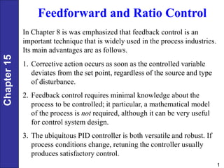
SlideShare a Scribd company logo
1 of 43
Chapter
15
1
Feedforward and Ratio Control
In Chapter 8 is was emphasized that feedback control is an
important technique that is widely used in the process industries.
Its main advantages are as follows.
1. Corrective action occurs as soon as the controlled variable
deviates from the set point, regardless of the source and type
of disturbance.
2. Feedback control requires minimal knowledge about the
process to be controlled; it particular, a mathematical model
of the process is not required, although it can be very useful
for control system design.
3. The ubiquitous PID controller is both versatile and robust. If
process conditions change, retuning the controller usually
produces satisfactory control.
Chapter
15
2
However, feedback control also has certain inherent
disadvantages:
1. No corrective action is taken until after a deviation in the
controlled variable occurs. Thus, perfect control, where the
controlled variable does not deviate from the set point during
disturbance or set-point changes, is theoretically impossible.
2. Feedback control does not provide predictive control action
to compensate for the effects of known or measurable
disturbances.
3. It may not be satisfactory for processes with large time
constants and/or long time delays. If large and frequent
disturbances occur, the process may operate continuously in a
transient state and never attain the desired steady state.
4. In some situations, the controlled variable cannot be
measured on-line, and, consequently, feedback control is not
feasible.
Chapter
15
3
Introduction to Feedforward Control
1. The disturbance variables must be measured on-line. In many
applications, this is not feasible.
2. To make effective use of feedforward control, at least a crude
process model should be available. In particular, we need to
know how the controlled variable responds to changes in both
the disturbance and manipulated variables. The quality of
feedforward control depends on the accuracy of the process
model.
3. Ideal feedforward controllers that are theoretically capable of
achieving perfect control may not be physically realizable.
Fortunately, practical approximations of these ideal controllers
often provide very effective control.
The basic concept of feedforward control is to measure important
disturbance variables and take corrective action before they upset
the process. Feedforward control has several disadvantages:
Chapter
15
4
Figure 15.2 The feedback control of the liquid level in a boiler
drum.
Chapter
15
5
• A boiler drum with a conventional feedback control system is
shown in Fig. 15.2. The level of the boiling liquid is measured
and used to adjust the feedwater flow rate.
• This control system tends to be quite sensitive to rapid changes
in the disturbance variable, steam flow rate, as a result of the
small liquid capacity of the boiler drum.
• Rapid disturbance changes can occur as a result of steam
demands made by downstream processing units.
The feedforward control scheme in Fig. 15.3 can provide better
control of the liquid level. Here the steam flow rate is
measured, and the feedforward controller adjusts the feedwater
flow rate.
Chapter
15
6
Figure 15.3 The feedforward control of the liquid level in a
boiler drum.
Chapter
15
7
Figure 15.4 The feedfoward-feedback control of the boiler
drum level.
Chapter
15
8
• In practical applications, feedforward control is normally used
in combination with feedback control.
• Feedforward control is used to reduce the effects of measurable
disturbances, while feedback trim compensates for inaccuracies
in the process model, measurement error, and unmeasured
disturbances.
Ratio control is a special type of feedforward control that has
had widespread application in the process industries. The
objective is to maintain the ratio of two process variables as a
specified value. The two variables are usually flow rates, a
manipulated variable u, and a disturbance variable d. Thus, the
ratio
is controlled rather than the individual variables. In Eq. 15-1, u
and d are physical variables, not deviation variables.
(15-1)
u
R
d

Ratio Control
Chapter
15
9
Typical applications of ratio control include:
1. Setting the relative amounts of components in blending
operations
2. Maintaining a stoichiometric ratio of reactants to a reactor
3. Keeping a specified reflux ratio for a distillation column
4. Holding the fuel-air ratio to a furnace at the optimum value.
Chapter
15
10
Figure 15.5 Ratio control, Method I.
Chapter
15
11
• The main advantage of Method I is that the actual ratio R is
calculated.
• A key disadvantage is that a divider element must be included
in the loop, and this element makes the process gain vary in a
nonlinear fashion. From Eq. 15-1, the process gain
1
(15-2)
p
d
R
K
u d

 
 
 

 
is inversely related to the disturbance flow rate . Because of
this significant disadvantage, the preferred scheme for
implementing ratio control is Method II, which is shown in
Fig. 15.6.
d
Chapter
15
12
Figure 15.6 Ratio control, Method II
Chapter
15
13
• Regardless of how ratio control is implemented, the process
variables must be scaled appropriately.
• For example, in Method II the gain setting for the ratio station
Kd must take into account the spans of the two flow
transmitters.
• Thus, the correct gain for the ratio station is
(15-3)
d
R d
u
S
K R
S

where Rd is the desired ratio, Su and Sd are the spans of the
flow transmitters for the manipulated and disturbance streams,
respectively.
Chapter
15
14
Example 15.1
A ratio control scheme is to be used to maintain a stoichoimetric
ratio of H2 and N2 as the feed to an ammonia synthesis reactor.
Individual flow controllers will be used for both the H2 and N2
streams. Using the information given below, do the following:
a) Draw a schematic diagram for the ratio control scheme.
b) Specify the appropriate gain for the ratio station, KR.
Chapter
15
15
Available Information
i. The electronic flow transmitters have built-in square root
extractors. The spans of the flow transmitters are 30 L/min for
H2 and 15 L/min for N2.
ii. The control valves have pneumatic actuators.
iii.Each required current-to-pressure (I/P) transducer has a gain
of 0.75 psi/mA.
iv. The ratio station is an electronic instrument with 4-20 mA
input and output signals.
Solution
The stoichiometric equation for the ammonia synthesis reaction is
2 2 3
3H N 2NH

Chapter
15
16
In order to introduce the feed mixture in stoichiometric
proportions, the ratio of the molar flow rates (H2/N2) should be
3:1. For the sake of simplicity, we assume that the ratio of the
molar flow rates is equal to the ratio of the volumetric flow rates.
But in general, the volumetric flow rates also depend on the
temperature and pressure of each stream (cf., the ideal gas law).
a) The schematic diagram for the ammonia synthesis reaction is
shown in Fig. 15.7. The H2 flow rate is considered to be the
disturbance variable, although this choice is arbitary because
both the H2 and N2 flow rates are controlled. Note that the ratio
station is merely a device with an adjustable gain. The input
signal to the ratio station is dm, the measured H2 flow rate. Its
output signal usp serves as the set point for the N2 flow control
loop. It is calculated as usp = KRdm.
Chapter
15
17
Figure 15.7 Ratio control scheme for an ammonia synthesis
reactor of Example 15.1
Chapter
15
18
b) From the stoichiometric equation, it follows that the desired
ratio is Rd = u/d = 1/3. Substitution into Equation 15-3 gives:
1 30 L/ min 2
3 15 L/ min 3
R
K
 
 
 
  
  
Feedforward Controller Design Based on
Steady-State Models
• A useful interpretation of feedforward control is that it
continually attempts to balance the material or energy that must
be delivered to the process against the demands of the load.
• For example, the level control system in Fig. 15.3 adjusts the
feedwater flow so that it balances the steam demand.
• Thus, it is natural to base the feedforward control calculations
on material and energy balances.
Chapter
15
19
Figure 15.8 A simple schematic diagram of a distillation
column.
Chapter
15
20
• To illustrate the design procedure, consider the distillation
column shown in Fig. 15.8 which is used to separate a binary
mixture.
• In Fig. 15.8, the symbols B, D, and F denote molar flow rates,
whereas x, y, and z are the mole fractions of the more volatile
component.
• The objective is to control the distillation composition, y,
despite measurable disturbances in feed flow rate F and feed
composition z, by adjusting distillate flow rate, D.
• It is assumed that measurements of x and y are not available.
The steady-state mass balances for the distillation column can be
written as
(15-4)
(15-5)
F D B
Fz Dy Bx
 
 
Chapter
15
21
Solving (15-4) for D and substituting into (15-5) gives
  (15-6)
F z x
D
y x



Because x and y are not measured, we replace these variables by
their set points to yield the feedforward control law:
  (15-7)
sp
sp sp
F z x
D
y x



Chapter
15
22
Blending System
• Consider the blending system and feedforward controller shown
in Fig. 15.9.
• We wish to design a feedforward control scheme to maintain
exit composition x at a constant set point xsp, despite
disturbances in inlet composition, x1.
• Suppose that inlet flow rate w1 and the composition of the other
inlet stream, x2, are constant.
• It is assumed that x1 is measured but x is not.
Chapter
15
23
Figure 15.9 Feedforward control of exit composition in the
blending system.
Chapter
15
24
The starting point for the feedforward controller design is the
steady-state mass and component balances,
1 2 (15-8)
w w w
 
1 1 2 2 (15-9)
wx w x w x
 
where the bar over the variable denotes a steady-state value.
Substituting Eq. 15-8 into 15-9 and solving for gives:
2
w
1 1
2
2
( )
(15-10)
w x x
w
x x



In order to derive a feedforward control law, we replace by xsp,
and and , by w2(t) and x1(t), respectively:
1 1
2
2
( )
( ) (15-11)
sp
sp
w x x t
w t
x x
 

 


Note that this feedforward control law is based on the physical
variables rather than on the deviation variables.
x
2
w 1
x
Chapter
15
25
• The feedforward control law in Eq. 15-11 is not in the final
form required for actual implementation because it ignores
two important instrumentation considerations:
• First, the actual value of x1 is not available but its measured
value, x1m, is.
• Second, the controller output signal is p rather than inlet flow
rate, w2.
• Thus, the feedforward control law should be expressed in
terms of x1m and p, rather than x1 and w2.
• Consequently, a more realistic feedforward control law should
incorporate the appropriate steady-state instrument relations
for the w2 flow transmitter and the control valve. (See text.)
Chapter
15
26
Feedforward Controller Design Based on
Dynamic Models
In this section, we consider the design of feedforward control
systems based on dynamic, rather than steady-state, process
models.
• As a starting point for our discussion, consider the block
diagram shown in Fig. 15.11.
• This diagram is similar to Fig. 11.8 for feedback control but
an additional signal path through Gt and Gf has been added.
Chapter
15
27
Figure 15.11 A block diagram of a feedforward-feedback control
system.
Chapter
15
28
The closed-loop transfer function for disturbance changes is:
 
 
(15-20)
1
d t f v p
c v p m
G G G G G
Y s
D s G G G G



Ideally, we would like the control system to produce perfect
control where the controlled variable remains exactly at the set
point despite arbitrary changes in the disturbance variable, D.
Thus, if the set point is constant (Ysp(s) = 0), we want Y(s) = 0,
even though D(s)
(15-21)
d
f
t v p
G
G
G G G
 
• Figure 15.11 and Eq. 15-21 provide a useful interpretation of the
ideal feedforward controller. Figure 15.11 indicates that a
disturbance has two effects.
• It upsets the process via the disturbance transfer function, Gd;
however, a corrective action is generated via the path through
GtGfGvGp.
Chapter
15
29
• Ideally, the corrective action compensates exactly for the upset
so that signals Yd and Yu cancel each other and Y(s) = 0.
Example 15.2
Suppose that
, (15-22)
τ 1 τ 1
p
d
d p
d p
K
K
G G
s s
 
 
Then from (15-22), the ideal feedforward controller is
τ 1
(15-23)
τ 1
p
d
f
t v p d
s
K
G
K K K s
  
 
   
  
 
 
This controller is a lead-lag unit with a gain given by
Kf = -Kd/KtKvKp. The dynamic response characteristics of lead-
lag units were considered in Example 6.1 of Chapter 6.
Chapter
15
30
Example 15.3
Now consider
From (15-21),
Because the term is a negative time delay, implying a
predictive element, the ideal feedforward controller in (15-25)
is physically unrealizable. However, we can approximate it by
omitting the term and increasing the value of the lead time
constant from to .
θ
, (15-24)
τ 1 τ 1
s
p
d
d p
d p
K e
K
G G
s s

 
 
θ
τ 1
(15-25)
τ 1
p s
d
f
t v p d
s
K
G e
K K K s

  
 
   
  
 
 
θs
e
θs
e
τp τ θ
p 
Chapter
15
31
Example 15.4
Finally, if
then the ideal feedforward controller,
is physically unrealizable because the numerator is a higher
order polynomial in s than the denominator. Again, we could
approximate this controller by a physically realizable one such
as a lead-lag unit, where the lead time constant is the sum of
the two time constants,
  
1 2
, (15-26)
1 1 1
p
d
d p
d p p
K
K
G G
s s s
  
 
  
  
 
1 2
τ 1 τ 1
(15-27)
τ 1
p p
d
f
t v p d
s s
K
G
K K K s
 
 
  
  
 
1 2
τ τ .
p p

Chapter
15
32
Stability Considerations
• To analyze the stability of the closed-loop system in Fig. 15.11,
we consider the closed-loop transfer function in Eq. 15-20.
• Setting the denominator equal to zero gives the characteristic
equation,
• In Chapter 11 it was shown that the roots of the characteristic
equation completely determine the stability of the closed-loop
system.
• Because Gf does not appear in the characteristic equation, the
feedforward controller has no effect on the stability of the
feedback control system.
• This is a desirable situation that allows the feedback and
feedforward controllers to be tuned individually.
1 0 (15-28)
c v p m
G G G G
 
Chapter
15
33
Lead-Lag Units
• The three examples in the previous section have demonstrated
that lead-lag units can provide reasonable approximations to
ideal feedforward controllers.
• Thus, if the feedforward controller consists of a lead-lag unit
with gain Kf, we can write
 
 
 
 
1
2
τ 1
(15-29)
τ 1
f
f
K s
U s
G s
D s s

 

Example 15.5
Consider the blending system of Section 15.3 and Fig. 15.9. A
feedforward-feedback control system is to be designed to reduce
the effect of disturbances in feed composition, x1, on the
controlled variable, produce composition, x. Inlet flow rate, w2,
can be manipulated. (See text.)
Chapter
15
34
Configurations for Feedforward-Feedback
Control
In a typical control configuration, the outputs of the feedforward
and feedback controllers are added together, and the sum is sent as
the signal to the final control element. Another useful
configuration for feedforward-feedback control is to have the
feedback controller output serve as the set point for the
feedforward controller.
Chapter
15
35
Figure 15.14 Feedforward-feedback control of exit composition in
the blending system.
Chapter
15
36
Figure 15.15 The open-
loop responses to step
changes in u and d.
Chapter
15
37
Tuning Feedforward Controllers
Feedforward controllers, like feedback controllers, usually
require tuning after installation in a plant.
Step 1. Adjust Kf.
• The effort required to tune a controller is greatly reduced if good
initial estimates of the controller parameters are available.
• An initial estimate of Kf can be obtained from a steady-state
model of the process or steady-state data.
• For example, suppose that the open-loop responses to step
changes in d and u are available, as shown in Fig. 15.15.
• After Kp and Kd have been determined, the feedforward
controller gain can be calculated from the steady-state version
of Eq. 15-22:
(15-40)
d
f
t v p
K
K
K K K
 
Chapter
15
38
• To tune the controller gain, Kf is set equal to an initial value, and
a small step change (3 to 5%) in the disturbance variable d is
introduced, if this is feasible.
• If an offset results, then Kf is adjusted until the offset is
eliminated.
• While Kf is being tuned, and should be set equal to their
minimum values, ideally zero.
1
τ 2
τ
Step 2. Determine initial values for and .
1
τ 2
τ
• Theoretical values for and can be calculated if a dynamic
model of the process is available, as shown in Example 15.2.
• Alternatively, initial estimates can be determined from open-
loop response data.
• For example, if the step responses have the shapes shown in
Figure 15.16, a reasonable process model is
1
τ 2
τ
Chapter
15
39
   
, (15-41)
τ 1 τ 1
p d
p d
p d
K K
G s G s
s s
 
 
where and can be calculated as shown in Fig. 15.16.
• A comparison of Eqs. 15-24 and 5-30 leads to the following
expression for and :
τp τd
1
τ 2
τ
1
τ τ (15-42)
p

2
τ τ (15-43)
d

• These values can then be used as initial estimates for the fine
tuning of and in Step 3.
• If neither a process model nor experimental data are
available, the relations or may be used,
depending on whether the controlled variable responds faster
to the load variable or to the manipulated variable.
1
τ 2
τ
1 2
τ / τ 2
 1 2
τ / τ 0.5

Chapter
15
40
•In view of Eq. 15-58, should be set equal to the estimated
dominant process time constant.
Step 3. Fine tune and .
• The final step is to use a trial-and-error procedure to fine tune
and by making small step changes in d.
• The desired step response consists of small deviations in the
controlled variable with equal areas above and below the set
point [1], as shown in Fig. 15.17.
• For simple process models, it can be proved theoretically that
equal areas above and below the set point imply that the
difference, , is correct (Exercise 15.8).
• In subsequent tuning to reduce the size of the areas, and
should be adjusted so that remains constant.
1
τ
1
τ 2
τ
1
τ
2
τ
1 2
τ τ

1
τ 2
τ
1 2
τ τ

Chapter
15
41
Figure 15.16 The desired response for a well-tuned feedforward
controller. (Note approximately equal areas above and below the
set point.)
Chapter
15
42
As a hypothetical illustration of this trial-and-error tuning
procedure, consider the set of responses shown in Fig. 15.17 for
positive step changes in disturbance variable d. It is assumed that
Kp > 0, Kd < 0, and controller gain Kf has already been adjusted so
that offset is eliminated.
Chapter
15
43
Figure 15.17 An example of feedforward controller tuning.

More Related Content

Similar to 1496818.ppt

Process control handout new1
Process control handout new1Process control handout new1
Process control handout new1Kiya Alemayehu
 
INSTRUMENTATION AND PROCESS CONTROL - BOILER CONTROL
INSTRUMENTATION AND PROCESS CONTROL - BOILER CONTROLINSTRUMENTATION AND PROCESS CONTROL - BOILER CONTROL
INSTRUMENTATION AND PROCESS CONTROL - BOILER CONTROLno suhaila
 
Implementation of closed loop control technique for improving the performance...
Implementation of closed loop control technique for improving the performance...Implementation of closed loop control technique for improving the performance...
Implementation of closed loop control technique for improving the performance...IJERA Editor
 
cascade and ratio control word doc
cascade and ratio control word doccascade and ratio control word doc
cascade and ratio control word docUmer Farooq
 
Multi objective control of nonlinear boiler-turbine dynamics with actuator ma...
Multi objective control of nonlinear boiler-turbine dynamics with actuator ma...Multi objective control of nonlinear boiler-turbine dynamics with actuator ma...
Multi objective control of nonlinear boiler-turbine dynamics with actuator ma...ISA Interchange
 
10.1.1.193.2962
10.1.1.193.296210.1.1.193.2962
10.1.1.193.2962aboma2hawi
 
Voltage Regulation of Boost Converter using Observer based Sliding Mode Contr...
Voltage Regulation of Boost Converter using Observer based Sliding Mode Contr...Voltage Regulation of Boost Converter using Observer based Sliding Mode Contr...
Voltage Regulation of Boost Converter using Observer based Sliding Mode Contr...TELKOMNIKA JOURNAL
 
MODELLING CASCADED SPLIT RANGE (CASC-SRC) CONTROLLERS IN ASPEN HYSYS DYNAMICS
MODELLING CASCADED SPLIT RANGE (CASC-SRC) CONTROLLERS IN ASPEN HYSYS DYNAMICSMODELLING CASCADED SPLIT RANGE (CASC-SRC) CONTROLLERS IN ASPEN HYSYS DYNAMICS
MODELLING CASCADED SPLIT RANGE (CASC-SRC) CONTROLLERS IN ASPEN HYSYS DYNAMICSVijay Sarathy
 
Flow measurement basics
Flow measurement basicsFlow measurement basics
Flow measurement basicsSalman1011
 
A STUDY ON PERFORMANCE OF DIFFERENT OPEN LOOP PID TUNNING TECHNIQUE FOR A LIQ...
A STUDY ON PERFORMANCE OF DIFFERENT OPEN LOOP PID TUNNING TECHNIQUE FOR A LIQ...A STUDY ON PERFORMANCE OF DIFFERENT OPEN LOOP PID TUNNING TECHNIQUE FOR A LIQ...
A STUDY ON PERFORMANCE OF DIFFERENT OPEN LOOP PID TUNNING TECHNIQUE FOR A LIQ...IJITCA Journal
 
A Study on Performance of Different Open Loop PID Tunning Technique for a Liq...
A Study on Performance of Different Open Loop PID Tunning Technique for a Liq...A Study on Performance of Different Open Loop PID Tunning Technique for a Liq...
A Study on Performance of Different Open Loop PID Tunning Technique for a Liq...IJITCA Journal
 
A STUDY ON PERFORMANCE OF DIFFERENT OPEN LOOP PID TUNNING TECHNIQUE FOR A LI...
A STUDY ON PERFORMANCE OF DIFFERENT OPEN LOOP  PID TUNNING TECHNIQUE FOR A LI...A STUDY ON PERFORMANCE OF DIFFERENT OPEN LOOP  PID TUNNING TECHNIQUE FOR A LI...
A STUDY ON PERFORMANCE OF DIFFERENT OPEN LOOP PID TUNNING TECHNIQUE FOR A LI...IJITCA Journal
 
K11619 rishabh jain
K11619 rishabh jainK11619 rishabh jain
K11619 rishabh jainRishabh Jain
 

Similar to 1496818.ppt (20)

Chapter_9.ppt
Chapter_9.pptChapter_9.ppt
Chapter_9.ppt
 
PID controller
PID controllerPID controller
PID controller
 
Chapter_8.ppt
Chapter_8.pptChapter_8.ppt
Chapter_8.ppt
 
3.CONTROL ACTIONS.pptx
3.CONTROL ACTIONS.pptx3.CONTROL ACTIONS.pptx
3.CONTROL ACTIONS.pptx
 
Process control handout new1
Process control handout new1Process control handout new1
Process control handout new1
 
INSTRUMENTATION AND PROCESS CONTROL - BOILER CONTROL
INSTRUMENTATION AND PROCESS CONTROL - BOILER CONTROLINSTRUMENTATION AND PROCESS CONTROL - BOILER CONTROL
INSTRUMENTATION AND PROCESS CONTROL - BOILER CONTROL
 
B035208015
B035208015B035208015
B035208015
 
Implementation of closed loop control technique for improving the performance...
Implementation of closed loop control technique for improving the performance...Implementation of closed loop control technique for improving the performance...
Implementation of closed loop control technique for improving the performance...
 
cascade and ratio control word doc
cascade and ratio control word doccascade and ratio control word doc
cascade and ratio control word doc
 
Multi objective control of nonlinear boiler-turbine dynamics with actuator ma...
Multi objective control of nonlinear boiler-turbine dynamics with actuator ma...Multi objective control of nonlinear boiler-turbine dynamics with actuator ma...
Multi objective control of nonlinear boiler-turbine dynamics with actuator ma...
 
Ch16_1_27_05.ppt
Ch16_1_27_05.pptCh16_1_27_05.ppt
Ch16_1_27_05.ppt
 
10.1.1.193.2962
10.1.1.193.296210.1.1.193.2962
10.1.1.193.2962
 
Control
ControlControl
Control
 
Voltage Regulation of Boost Converter using Observer based Sliding Mode Contr...
Voltage Regulation of Boost Converter using Observer based Sliding Mode Contr...Voltage Regulation of Boost Converter using Observer based Sliding Mode Contr...
Voltage Regulation of Boost Converter using Observer based Sliding Mode Contr...
 
MODELLING CASCADED SPLIT RANGE (CASC-SRC) CONTROLLERS IN ASPEN HYSYS DYNAMICS
MODELLING CASCADED SPLIT RANGE (CASC-SRC) CONTROLLERS IN ASPEN HYSYS DYNAMICSMODELLING CASCADED SPLIT RANGE (CASC-SRC) CONTROLLERS IN ASPEN HYSYS DYNAMICS
MODELLING CASCADED SPLIT RANGE (CASC-SRC) CONTROLLERS IN ASPEN HYSYS DYNAMICS
 
Flow measurement basics
Flow measurement basicsFlow measurement basics
Flow measurement basics
 
A STUDY ON PERFORMANCE OF DIFFERENT OPEN LOOP PID TUNNING TECHNIQUE FOR A LIQ...
A STUDY ON PERFORMANCE OF DIFFERENT OPEN LOOP PID TUNNING TECHNIQUE FOR A LIQ...A STUDY ON PERFORMANCE OF DIFFERENT OPEN LOOP PID TUNNING TECHNIQUE FOR A LIQ...
A STUDY ON PERFORMANCE OF DIFFERENT OPEN LOOP PID TUNNING TECHNIQUE FOR A LIQ...
 
A Study on Performance of Different Open Loop PID Tunning Technique for a Liq...
A Study on Performance of Different Open Loop PID Tunning Technique for a Liq...A Study on Performance of Different Open Loop PID Tunning Technique for a Liq...
A Study on Performance of Different Open Loop PID Tunning Technique for a Liq...
 
A STUDY ON PERFORMANCE OF DIFFERENT OPEN LOOP PID TUNNING TECHNIQUE FOR A LI...
A STUDY ON PERFORMANCE OF DIFFERENT OPEN LOOP  PID TUNNING TECHNIQUE FOR A LI...A STUDY ON PERFORMANCE OF DIFFERENT OPEN LOOP  PID TUNNING TECHNIQUE FOR A LI...
A STUDY ON PERFORMANCE OF DIFFERENT OPEN LOOP PID TUNNING TECHNIQUE FOR A LI...
 
K11619 rishabh jain
K11619 rishabh jainK11619 rishabh jain
K11619 rishabh jain
 

More from MuhammadMubeen58 (12)

3603939.ppt
3603939.ppt3603939.ppt
3603939.ppt
 
3330716.ppt
3330716.ppt3330716.ppt
3330716.ppt
 
2760114.ppt
2760114.ppt2760114.ppt
2760114.ppt
 
2706264.ppt
2706264.ppt2706264.ppt
2706264.ppt
 
1619494.ppt
1619494.ppt1619494.ppt
1619494.ppt
 
1578385.ppt
1578385.ppt1578385.ppt
1578385.ppt
 
1577320.ppt
1577320.ppt1577320.ppt
1577320.ppt
 
1474058.ppt
1474058.ppt1474058.ppt
1474058.ppt
 
1413570.ppt
1413570.ppt1413570.ppt
1413570.ppt
 
223296.ppt
223296.ppt223296.ppt
223296.ppt
 
14446351.ppt
14446351.ppt14446351.ppt
14446351.ppt
 
4470838.ppt
4470838.ppt4470838.ppt
4470838.ppt
 

Recently uploaded

Microscopic Analysis of Ceramic Materials.pptx
Microscopic Analysis of Ceramic Materials.pptxMicroscopic Analysis of Ceramic Materials.pptx
Microscopic Analysis of Ceramic Materials.pptxpurnimasatapathy1234
 
Top Rated Pune Call Girls Budhwar Peth ⟟ 6297143586 ⟟ Call Me For Genuine Se...
Top Rated  Pune Call Girls Budhwar Peth ⟟ 6297143586 ⟟ Call Me For Genuine Se...Top Rated  Pune Call Girls Budhwar Peth ⟟ 6297143586 ⟟ Call Me For Genuine Se...
Top Rated Pune Call Girls Budhwar Peth ⟟ 6297143586 ⟟ Call Me For Genuine Se...Call Girls in Nagpur High Profile
 
VIP Call Girls Service Hitech City Hyderabad Call +91-8250192130
VIP Call Girls Service Hitech City Hyderabad Call +91-8250192130VIP Call Girls Service Hitech City Hyderabad Call +91-8250192130
VIP Call Girls Service Hitech City Hyderabad Call +91-8250192130Suhani Kapoor
 
OSVC_Meta-Data based Simulation Automation to overcome Verification Challenge...
OSVC_Meta-Data based Simulation Automation to overcome Verification Challenge...OSVC_Meta-Data based Simulation Automation to overcome Verification Challenge...
OSVC_Meta-Data based Simulation Automation to overcome Verification Challenge...Soham Mondal
 
MANUFACTURING PROCESS-II UNIT-2 LATHE MACHINE
MANUFACTURING PROCESS-II UNIT-2 LATHE MACHINEMANUFACTURING PROCESS-II UNIT-2 LATHE MACHINE
MANUFACTURING PROCESS-II UNIT-2 LATHE MACHINESIVASHANKAR N
 
The Most Attractive Pune Call Girls Budhwar Peth 8250192130 Will You Miss Thi...
The Most Attractive Pune Call Girls Budhwar Peth 8250192130 Will You Miss Thi...The Most Attractive Pune Call Girls Budhwar Peth 8250192130 Will You Miss Thi...
The Most Attractive Pune Call Girls Budhwar Peth 8250192130 Will You Miss Thi...ranjana rawat
 
(RIA) Call Girls Bhosari ( 7001035870 ) HI-Fi Pune Escorts Service
(RIA) Call Girls Bhosari ( 7001035870 ) HI-Fi Pune Escorts Service(RIA) Call Girls Bhosari ( 7001035870 ) HI-Fi Pune Escorts Service
(RIA) Call Girls Bhosari ( 7001035870 ) HI-Fi Pune Escorts Serviceranjana rawat
 
College Call Girls Nashik Nehal 7001305949 Independent Escort Service Nashik
College Call Girls Nashik Nehal 7001305949 Independent Escort Service NashikCollege Call Girls Nashik Nehal 7001305949 Independent Escort Service Nashik
College Call Girls Nashik Nehal 7001305949 Independent Escort Service NashikCall Girls in Nagpur High Profile
 
Extrusion Processes and Their Limitations
Extrusion Processes and Their LimitationsExtrusion Processes and Their Limitations
Extrusion Processes and Their Limitations120cr0395
 
IMPLICATIONS OF THE ABOVE HOLISTIC UNDERSTANDING OF HARMONY ON PROFESSIONAL E...
IMPLICATIONS OF THE ABOVE HOLISTIC UNDERSTANDING OF HARMONY ON PROFESSIONAL E...IMPLICATIONS OF THE ABOVE HOLISTIC UNDERSTANDING OF HARMONY ON PROFESSIONAL E...
IMPLICATIONS OF THE ABOVE HOLISTIC UNDERSTANDING OF HARMONY ON PROFESSIONAL E...RajaP95
 
Introduction to IEEE STANDARDS and its different types.pptx
Introduction to IEEE STANDARDS and its different types.pptxIntroduction to IEEE STANDARDS and its different types.pptx
Introduction to IEEE STANDARDS and its different types.pptxupamatechverse
 
Call Girls Service Nagpur Tanvi Call 7001035870 Meet With Nagpur Escorts
Call Girls Service Nagpur Tanvi Call 7001035870 Meet With Nagpur EscortsCall Girls Service Nagpur Tanvi Call 7001035870 Meet With Nagpur Escorts
Call Girls Service Nagpur Tanvi Call 7001035870 Meet With Nagpur EscortsCall Girls in Nagpur High Profile
 
(SHREYA) Chakan Call Girls Just Call 7001035870 [ Cash on Delivery ] Pune Esc...
(SHREYA) Chakan Call Girls Just Call 7001035870 [ Cash on Delivery ] Pune Esc...(SHREYA) Chakan Call Girls Just Call 7001035870 [ Cash on Delivery ] Pune Esc...
(SHREYA) Chakan Call Girls Just Call 7001035870 [ Cash on Delivery ] Pune Esc...ranjana rawat
 
UNIT - IV - Air Compressors and its Performance
UNIT - IV - Air Compressors and its PerformanceUNIT - IV - Air Compressors and its Performance
UNIT - IV - Air Compressors and its Performancesivaprakash250
 
CCS335 _ Neural Networks and Deep Learning Laboratory_Lab Complete Record
CCS335 _ Neural Networks and Deep Learning Laboratory_Lab Complete RecordCCS335 _ Neural Networks and Deep Learning Laboratory_Lab Complete Record
CCS335 _ Neural Networks and Deep Learning Laboratory_Lab Complete RecordAsst.prof M.Gokilavani
 
Porous Ceramics seminar and technical writing
Porous Ceramics seminar and technical writingPorous Ceramics seminar and technical writing
Porous Ceramics seminar and technical writingrakeshbaidya232001
 
HARDNESS, FRACTURE TOUGHNESS AND STRENGTH OF CERAMICS
HARDNESS, FRACTURE TOUGHNESS AND STRENGTH OF CERAMICSHARDNESS, FRACTURE TOUGHNESS AND STRENGTH OF CERAMICS
HARDNESS, FRACTURE TOUGHNESS AND STRENGTH OF CERAMICSRajkumarAkumalla
 

Recently uploaded (20)

Microscopic Analysis of Ceramic Materials.pptx
Microscopic Analysis of Ceramic Materials.pptxMicroscopic Analysis of Ceramic Materials.pptx
Microscopic Analysis of Ceramic Materials.pptx
 
Top Rated Pune Call Girls Budhwar Peth ⟟ 6297143586 ⟟ Call Me For Genuine Se...
Top Rated  Pune Call Girls Budhwar Peth ⟟ 6297143586 ⟟ Call Me For Genuine Se...Top Rated  Pune Call Girls Budhwar Peth ⟟ 6297143586 ⟟ Call Me For Genuine Se...
Top Rated Pune Call Girls Budhwar Peth ⟟ 6297143586 ⟟ Call Me For Genuine Se...
 
VIP Call Girls Service Hitech City Hyderabad Call +91-8250192130
VIP Call Girls Service Hitech City Hyderabad Call +91-8250192130VIP Call Girls Service Hitech City Hyderabad Call +91-8250192130
VIP Call Girls Service Hitech City Hyderabad Call +91-8250192130
 
OSVC_Meta-Data based Simulation Automation to overcome Verification Challenge...
OSVC_Meta-Data based Simulation Automation to overcome Verification Challenge...OSVC_Meta-Data based Simulation Automation to overcome Verification Challenge...
OSVC_Meta-Data based Simulation Automation to overcome Verification Challenge...
 
MANUFACTURING PROCESS-II UNIT-2 LATHE MACHINE
MANUFACTURING PROCESS-II UNIT-2 LATHE MACHINEMANUFACTURING PROCESS-II UNIT-2 LATHE MACHINE
MANUFACTURING PROCESS-II UNIT-2 LATHE MACHINE
 
The Most Attractive Pune Call Girls Budhwar Peth 8250192130 Will You Miss Thi...
The Most Attractive Pune Call Girls Budhwar Peth 8250192130 Will You Miss Thi...The Most Attractive Pune Call Girls Budhwar Peth 8250192130 Will You Miss Thi...
The Most Attractive Pune Call Girls Budhwar Peth 8250192130 Will You Miss Thi...
 
(RIA) Call Girls Bhosari ( 7001035870 ) HI-Fi Pune Escorts Service
(RIA) Call Girls Bhosari ( 7001035870 ) HI-Fi Pune Escorts Service(RIA) Call Girls Bhosari ( 7001035870 ) HI-Fi Pune Escorts Service
(RIA) Call Girls Bhosari ( 7001035870 ) HI-Fi Pune Escorts Service
 
★ CALL US 9953330565 ( HOT Young Call Girls In Badarpur delhi NCR
★ CALL US 9953330565 ( HOT Young Call Girls In Badarpur delhi NCR★ CALL US 9953330565 ( HOT Young Call Girls In Badarpur delhi NCR
★ CALL US 9953330565 ( HOT Young Call Girls In Badarpur delhi NCR
 
College Call Girls Nashik Nehal 7001305949 Independent Escort Service Nashik
College Call Girls Nashik Nehal 7001305949 Independent Escort Service NashikCollege Call Girls Nashik Nehal 7001305949 Independent Escort Service Nashik
College Call Girls Nashik Nehal 7001305949 Independent Escort Service Nashik
 
Extrusion Processes and Their Limitations
Extrusion Processes and Their LimitationsExtrusion Processes and Their Limitations
Extrusion Processes and Their Limitations
 
IMPLICATIONS OF THE ABOVE HOLISTIC UNDERSTANDING OF HARMONY ON PROFESSIONAL E...
IMPLICATIONS OF THE ABOVE HOLISTIC UNDERSTANDING OF HARMONY ON PROFESSIONAL E...IMPLICATIONS OF THE ABOVE HOLISTIC UNDERSTANDING OF HARMONY ON PROFESSIONAL E...
IMPLICATIONS OF THE ABOVE HOLISTIC UNDERSTANDING OF HARMONY ON PROFESSIONAL E...
 
Introduction to IEEE STANDARDS and its different types.pptx
Introduction to IEEE STANDARDS and its different types.pptxIntroduction to IEEE STANDARDS and its different types.pptx
Introduction to IEEE STANDARDS and its different types.pptx
 
Call Girls Service Nagpur Tanvi Call 7001035870 Meet With Nagpur Escorts
Call Girls Service Nagpur Tanvi Call 7001035870 Meet With Nagpur EscortsCall Girls Service Nagpur Tanvi Call 7001035870 Meet With Nagpur Escorts
Call Girls Service Nagpur Tanvi Call 7001035870 Meet With Nagpur Escorts
 
(SHREYA) Chakan Call Girls Just Call 7001035870 [ Cash on Delivery ] Pune Esc...
(SHREYA) Chakan Call Girls Just Call 7001035870 [ Cash on Delivery ] Pune Esc...(SHREYA) Chakan Call Girls Just Call 7001035870 [ Cash on Delivery ] Pune Esc...
(SHREYA) Chakan Call Girls Just Call 7001035870 [ Cash on Delivery ] Pune Esc...
 
UNIT - IV - Air Compressors and its Performance
UNIT - IV - Air Compressors and its PerformanceUNIT - IV - Air Compressors and its Performance
UNIT - IV - Air Compressors and its Performance
 
CCS335 _ Neural Networks and Deep Learning Laboratory_Lab Complete Record
CCS335 _ Neural Networks and Deep Learning Laboratory_Lab Complete RecordCCS335 _ Neural Networks and Deep Learning Laboratory_Lab Complete Record
CCS335 _ Neural Networks and Deep Learning Laboratory_Lab Complete Record
 
Porous Ceramics seminar and technical writing
Porous Ceramics seminar and technical writingPorous Ceramics seminar and technical writing
Porous Ceramics seminar and technical writing
 
HARDNESS, FRACTURE TOUGHNESS AND STRENGTH OF CERAMICS
HARDNESS, FRACTURE TOUGHNESS AND STRENGTH OF CERAMICSHARDNESS, FRACTURE TOUGHNESS AND STRENGTH OF CERAMICS
HARDNESS, FRACTURE TOUGHNESS AND STRENGTH OF CERAMICS
 
DJARUM4D - SLOT GACOR ONLINE | SLOT DEMO ONLINE
DJARUM4D - SLOT GACOR ONLINE | SLOT DEMO ONLINEDJARUM4D - SLOT GACOR ONLINE | SLOT DEMO ONLINE
DJARUM4D - SLOT GACOR ONLINE | SLOT DEMO ONLINE
 
Roadmap to Membership of RICS - Pathways and Routes
Roadmap to Membership of RICS - Pathways and RoutesRoadmap to Membership of RICS - Pathways and Routes
Roadmap to Membership of RICS - Pathways and Routes
 

1496818.ppt

  • 1. Chapter 15 1 Feedforward and Ratio Control In Chapter 8 is was emphasized that feedback control is an important technique that is widely used in the process industries. Its main advantages are as follows. 1. Corrective action occurs as soon as the controlled variable deviates from the set point, regardless of the source and type of disturbance. 2. Feedback control requires minimal knowledge about the process to be controlled; it particular, a mathematical model of the process is not required, although it can be very useful for control system design. 3. The ubiquitous PID controller is both versatile and robust. If process conditions change, retuning the controller usually produces satisfactory control.
  • 2. Chapter 15 2 However, feedback control also has certain inherent disadvantages: 1. No corrective action is taken until after a deviation in the controlled variable occurs. Thus, perfect control, where the controlled variable does not deviate from the set point during disturbance or set-point changes, is theoretically impossible. 2. Feedback control does not provide predictive control action to compensate for the effects of known or measurable disturbances. 3. It may not be satisfactory for processes with large time constants and/or long time delays. If large and frequent disturbances occur, the process may operate continuously in a transient state and never attain the desired steady state. 4. In some situations, the controlled variable cannot be measured on-line, and, consequently, feedback control is not feasible.
  • 3. Chapter 15 3 Introduction to Feedforward Control 1. The disturbance variables must be measured on-line. In many applications, this is not feasible. 2. To make effective use of feedforward control, at least a crude process model should be available. In particular, we need to know how the controlled variable responds to changes in both the disturbance and manipulated variables. The quality of feedforward control depends on the accuracy of the process model. 3. Ideal feedforward controllers that are theoretically capable of achieving perfect control may not be physically realizable. Fortunately, practical approximations of these ideal controllers often provide very effective control. The basic concept of feedforward control is to measure important disturbance variables and take corrective action before they upset the process. Feedforward control has several disadvantages:
  • 4. Chapter 15 4 Figure 15.2 The feedback control of the liquid level in a boiler drum.
  • 5. Chapter 15 5 • A boiler drum with a conventional feedback control system is shown in Fig. 15.2. The level of the boiling liquid is measured and used to adjust the feedwater flow rate. • This control system tends to be quite sensitive to rapid changes in the disturbance variable, steam flow rate, as a result of the small liquid capacity of the boiler drum. • Rapid disturbance changes can occur as a result of steam demands made by downstream processing units. The feedforward control scheme in Fig. 15.3 can provide better control of the liquid level. Here the steam flow rate is measured, and the feedforward controller adjusts the feedwater flow rate.
  • 6. Chapter 15 6 Figure 15.3 The feedforward control of the liquid level in a boiler drum.
  • 7. Chapter 15 7 Figure 15.4 The feedfoward-feedback control of the boiler drum level.
  • 8. Chapter 15 8 • In practical applications, feedforward control is normally used in combination with feedback control. • Feedforward control is used to reduce the effects of measurable disturbances, while feedback trim compensates for inaccuracies in the process model, measurement error, and unmeasured disturbances. Ratio control is a special type of feedforward control that has had widespread application in the process industries. The objective is to maintain the ratio of two process variables as a specified value. The two variables are usually flow rates, a manipulated variable u, and a disturbance variable d. Thus, the ratio is controlled rather than the individual variables. In Eq. 15-1, u and d are physical variables, not deviation variables. (15-1) u R d  Ratio Control
  • 9. Chapter 15 9 Typical applications of ratio control include: 1. Setting the relative amounts of components in blending operations 2. Maintaining a stoichiometric ratio of reactants to a reactor 3. Keeping a specified reflux ratio for a distillation column 4. Holding the fuel-air ratio to a furnace at the optimum value.
  • 10. Chapter 15 10 Figure 15.5 Ratio control, Method I.
  • 11. Chapter 15 11 • The main advantage of Method I is that the actual ratio R is calculated. • A key disadvantage is that a divider element must be included in the loop, and this element makes the process gain vary in a nonlinear fashion. From Eq. 15-1, the process gain 1 (15-2) p d R K u d           is inversely related to the disturbance flow rate . Because of this significant disadvantage, the preferred scheme for implementing ratio control is Method II, which is shown in Fig. 15.6. d
  • 12. Chapter 15 12 Figure 15.6 Ratio control, Method II
  • 13. Chapter 15 13 • Regardless of how ratio control is implemented, the process variables must be scaled appropriately. • For example, in Method II the gain setting for the ratio station Kd must take into account the spans of the two flow transmitters. • Thus, the correct gain for the ratio station is (15-3) d R d u S K R S  where Rd is the desired ratio, Su and Sd are the spans of the flow transmitters for the manipulated and disturbance streams, respectively.
  • 14. Chapter 15 14 Example 15.1 A ratio control scheme is to be used to maintain a stoichoimetric ratio of H2 and N2 as the feed to an ammonia synthesis reactor. Individual flow controllers will be used for both the H2 and N2 streams. Using the information given below, do the following: a) Draw a schematic diagram for the ratio control scheme. b) Specify the appropriate gain for the ratio station, KR.
  • 15. Chapter 15 15 Available Information i. The electronic flow transmitters have built-in square root extractors. The spans of the flow transmitters are 30 L/min for H2 and 15 L/min for N2. ii. The control valves have pneumatic actuators. iii.Each required current-to-pressure (I/P) transducer has a gain of 0.75 psi/mA. iv. The ratio station is an electronic instrument with 4-20 mA input and output signals. Solution The stoichiometric equation for the ammonia synthesis reaction is 2 2 3 3H N 2NH 
  • 16. Chapter 15 16 In order to introduce the feed mixture in stoichiometric proportions, the ratio of the molar flow rates (H2/N2) should be 3:1. For the sake of simplicity, we assume that the ratio of the molar flow rates is equal to the ratio of the volumetric flow rates. But in general, the volumetric flow rates also depend on the temperature and pressure of each stream (cf., the ideal gas law). a) The schematic diagram for the ammonia synthesis reaction is shown in Fig. 15.7. The H2 flow rate is considered to be the disturbance variable, although this choice is arbitary because both the H2 and N2 flow rates are controlled. Note that the ratio station is merely a device with an adjustable gain. The input signal to the ratio station is dm, the measured H2 flow rate. Its output signal usp serves as the set point for the N2 flow control loop. It is calculated as usp = KRdm.
  • 17. Chapter 15 17 Figure 15.7 Ratio control scheme for an ammonia synthesis reactor of Example 15.1
  • 18. Chapter 15 18 b) From the stoichiometric equation, it follows that the desired ratio is Rd = u/d = 1/3. Substitution into Equation 15-3 gives: 1 30 L/ min 2 3 15 L/ min 3 R K             Feedforward Controller Design Based on Steady-State Models • A useful interpretation of feedforward control is that it continually attempts to balance the material or energy that must be delivered to the process against the demands of the load. • For example, the level control system in Fig. 15.3 adjusts the feedwater flow so that it balances the steam demand. • Thus, it is natural to base the feedforward control calculations on material and energy balances.
  • 19. Chapter 15 19 Figure 15.8 A simple schematic diagram of a distillation column.
  • 20. Chapter 15 20 • To illustrate the design procedure, consider the distillation column shown in Fig. 15.8 which is used to separate a binary mixture. • In Fig. 15.8, the symbols B, D, and F denote molar flow rates, whereas x, y, and z are the mole fractions of the more volatile component. • The objective is to control the distillation composition, y, despite measurable disturbances in feed flow rate F and feed composition z, by adjusting distillate flow rate, D. • It is assumed that measurements of x and y are not available. The steady-state mass balances for the distillation column can be written as (15-4) (15-5) F D B Fz Dy Bx    
  • 21. Chapter 15 21 Solving (15-4) for D and substituting into (15-5) gives   (15-6) F z x D y x    Because x and y are not measured, we replace these variables by their set points to yield the feedforward control law:   (15-7) sp sp sp F z x D y x   
  • 22. Chapter 15 22 Blending System • Consider the blending system and feedforward controller shown in Fig. 15.9. • We wish to design a feedforward control scheme to maintain exit composition x at a constant set point xsp, despite disturbances in inlet composition, x1. • Suppose that inlet flow rate w1 and the composition of the other inlet stream, x2, are constant. • It is assumed that x1 is measured but x is not.
  • 23. Chapter 15 23 Figure 15.9 Feedforward control of exit composition in the blending system.
  • 24. Chapter 15 24 The starting point for the feedforward controller design is the steady-state mass and component balances, 1 2 (15-8) w w w   1 1 2 2 (15-9) wx w x w x   where the bar over the variable denotes a steady-state value. Substituting Eq. 15-8 into 15-9 and solving for gives: 2 w 1 1 2 2 ( ) (15-10) w x x w x x    In order to derive a feedforward control law, we replace by xsp, and and , by w2(t) and x1(t), respectively: 1 1 2 2 ( ) ( ) (15-11) sp sp w x x t w t x x        Note that this feedforward control law is based on the physical variables rather than on the deviation variables. x 2 w 1 x
  • 25. Chapter 15 25 • The feedforward control law in Eq. 15-11 is not in the final form required for actual implementation because it ignores two important instrumentation considerations: • First, the actual value of x1 is not available but its measured value, x1m, is. • Second, the controller output signal is p rather than inlet flow rate, w2. • Thus, the feedforward control law should be expressed in terms of x1m and p, rather than x1 and w2. • Consequently, a more realistic feedforward control law should incorporate the appropriate steady-state instrument relations for the w2 flow transmitter and the control valve. (See text.)
  • 26. Chapter 15 26 Feedforward Controller Design Based on Dynamic Models In this section, we consider the design of feedforward control systems based on dynamic, rather than steady-state, process models. • As a starting point for our discussion, consider the block diagram shown in Fig. 15.11. • This diagram is similar to Fig. 11.8 for feedback control but an additional signal path through Gt and Gf has been added.
  • 27. Chapter 15 27 Figure 15.11 A block diagram of a feedforward-feedback control system.
  • 28. Chapter 15 28 The closed-loop transfer function for disturbance changes is:     (15-20) 1 d t f v p c v p m G G G G G Y s D s G G G G    Ideally, we would like the control system to produce perfect control where the controlled variable remains exactly at the set point despite arbitrary changes in the disturbance variable, D. Thus, if the set point is constant (Ysp(s) = 0), we want Y(s) = 0, even though D(s) (15-21) d f t v p G G G G G   • Figure 15.11 and Eq. 15-21 provide a useful interpretation of the ideal feedforward controller. Figure 15.11 indicates that a disturbance has two effects. • It upsets the process via the disturbance transfer function, Gd; however, a corrective action is generated via the path through GtGfGvGp.
  • 29. Chapter 15 29 • Ideally, the corrective action compensates exactly for the upset so that signals Yd and Yu cancel each other and Y(s) = 0. Example 15.2 Suppose that , (15-22) τ 1 τ 1 p d d p d p K K G G s s     Then from (15-22), the ideal feedforward controller is τ 1 (15-23) τ 1 p d f t v p d s K G K K K s                 This controller is a lead-lag unit with a gain given by Kf = -Kd/KtKvKp. The dynamic response characteristics of lead- lag units were considered in Example 6.1 of Chapter 6.
  • 30. Chapter 15 30 Example 15.3 Now consider From (15-21), Because the term is a negative time delay, implying a predictive element, the ideal feedforward controller in (15-25) is physically unrealizable. However, we can approximate it by omitting the term and increasing the value of the lead time constant from to . θ , (15-24) τ 1 τ 1 s p d d p d p K e K G G s s      θ τ 1 (15-25) τ 1 p s d f t v p d s K G e K K K s                  θs e θs e τp τ θ p 
  • 31. Chapter 15 31 Example 15.4 Finally, if then the ideal feedforward controller, is physically unrealizable because the numerator is a higher order polynomial in s than the denominator. Again, we could approximate this controller by a physically realizable one such as a lead-lag unit, where the lead time constant is the sum of the two time constants,    1 2 , (15-26) 1 1 1 p d d p d p p K K G G s s s              1 2 τ 1 τ 1 (15-27) τ 1 p p d f t v p d s s K G K K K s             1 2 τ τ . p p 
  • 32. Chapter 15 32 Stability Considerations • To analyze the stability of the closed-loop system in Fig. 15.11, we consider the closed-loop transfer function in Eq. 15-20. • Setting the denominator equal to zero gives the characteristic equation, • In Chapter 11 it was shown that the roots of the characteristic equation completely determine the stability of the closed-loop system. • Because Gf does not appear in the characteristic equation, the feedforward controller has no effect on the stability of the feedback control system. • This is a desirable situation that allows the feedback and feedforward controllers to be tuned individually. 1 0 (15-28) c v p m G G G G  
  • 33. Chapter 15 33 Lead-Lag Units • The three examples in the previous section have demonstrated that lead-lag units can provide reasonable approximations to ideal feedforward controllers. • Thus, if the feedforward controller consists of a lead-lag unit with gain Kf, we can write         1 2 τ 1 (15-29) τ 1 f f K s U s G s D s s     Example 15.5 Consider the blending system of Section 15.3 and Fig. 15.9. A feedforward-feedback control system is to be designed to reduce the effect of disturbances in feed composition, x1, on the controlled variable, produce composition, x. Inlet flow rate, w2, can be manipulated. (See text.)
  • 34. Chapter 15 34 Configurations for Feedforward-Feedback Control In a typical control configuration, the outputs of the feedforward and feedback controllers are added together, and the sum is sent as the signal to the final control element. Another useful configuration for feedforward-feedback control is to have the feedback controller output serve as the set point for the feedforward controller.
  • 35. Chapter 15 35 Figure 15.14 Feedforward-feedback control of exit composition in the blending system.
  • 36. Chapter 15 36 Figure 15.15 The open- loop responses to step changes in u and d.
  • 37. Chapter 15 37 Tuning Feedforward Controllers Feedforward controllers, like feedback controllers, usually require tuning after installation in a plant. Step 1. Adjust Kf. • The effort required to tune a controller is greatly reduced if good initial estimates of the controller parameters are available. • An initial estimate of Kf can be obtained from a steady-state model of the process or steady-state data. • For example, suppose that the open-loop responses to step changes in d and u are available, as shown in Fig. 15.15. • After Kp and Kd have been determined, the feedforward controller gain can be calculated from the steady-state version of Eq. 15-22: (15-40) d f t v p K K K K K  
  • 38. Chapter 15 38 • To tune the controller gain, Kf is set equal to an initial value, and a small step change (3 to 5%) in the disturbance variable d is introduced, if this is feasible. • If an offset results, then Kf is adjusted until the offset is eliminated. • While Kf is being tuned, and should be set equal to their minimum values, ideally zero. 1 τ 2 τ Step 2. Determine initial values for and . 1 τ 2 τ • Theoretical values for and can be calculated if a dynamic model of the process is available, as shown in Example 15.2. • Alternatively, initial estimates can be determined from open- loop response data. • For example, if the step responses have the shapes shown in Figure 15.16, a reasonable process model is 1 τ 2 τ
  • 39. Chapter 15 39     , (15-41) τ 1 τ 1 p d p d p d K K G s G s s s     where and can be calculated as shown in Fig. 15.16. • A comparison of Eqs. 15-24 and 5-30 leads to the following expression for and : τp τd 1 τ 2 τ 1 τ τ (15-42) p  2 τ τ (15-43) d  • These values can then be used as initial estimates for the fine tuning of and in Step 3. • If neither a process model nor experimental data are available, the relations or may be used, depending on whether the controlled variable responds faster to the load variable or to the manipulated variable. 1 τ 2 τ 1 2 τ / τ 2  1 2 τ / τ 0.5 
  • 40. Chapter 15 40 •In view of Eq. 15-58, should be set equal to the estimated dominant process time constant. Step 3. Fine tune and . • The final step is to use a trial-and-error procedure to fine tune and by making small step changes in d. • The desired step response consists of small deviations in the controlled variable with equal areas above and below the set point [1], as shown in Fig. 15.17. • For simple process models, it can be proved theoretically that equal areas above and below the set point imply that the difference, , is correct (Exercise 15.8). • In subsequent tuning to reduce the size of the areas, and should be adjusted so that remains constant. 1 τ 1 τ 2 τ 1 τ 2 τ 1 2 τ τ  1 τ 2 τ 1 2 τ τ 
  • 41. Chapter 15 41 Figure 15.16 The desired response for a well-tuned feedforward controller. (Note approximately equal areas above and below the set point.)
  • 42. Chapter 15 42 As a hypothetical illustration of this trial-and-error tuning procedure, consider the set of responses shown in Fig. 15.17 for positive step changes in disturbance variable d. It is assumed that Kp > 0, Kd < 0, and controller gain Kf has already been adjusted so that offset is eliminated.
  • 43. Chapter 15 43 Figure 15.17 An example of feedforward controller tuning.