![CONTROL ENGINEERING
Course Code 18ME71 CIE Marks 40
Teaching Hours / Week (L:T:P) 3:0:0 SEE Marks 60
Credits 03 Exam Hours 03
[AS PER CHOICE BASED CREDIT SYSTEM (CBCS) SCHEME]
SEMESTER – VII
Dr. Mohammed Imran
B. E. IN MECHANICAL ENGINEERING](https://image.slidesharecdn.com/controlengineeringmodule-2-220109134221/85/Control-engineering-module-2-18ME71-PPT-Cum-Notes-1-320.jpg)
![CONTROL ENGINEERING
Course Code 18ME71 CIE Marks 40
Teaching Hours / Week (L:T:P) 3:0:0 SEE Marks 60
Credits 03 Exam Hours 03
[AS PER CHOICE BASED CREDIT SYSTEM (CBCS) SCHEME]
SEMESTER – VII
Dr. Mohammed Imran
B. E. IN MECHANICAL ENGINEERING](https://image.slidesharecdn.com/controlengineeringmodule-2-220109134221/75/Control-engineering-module-2-18ME71-PPT-Cum-Notes-1-2048.jpg)
![CONTROL ENGINEERING
Course Code 18ME71 CIE Marks 40
Teaching Hours / Week (L:T:P) 3:0:0 SEE Marks 60
Credits 03 Exam Hours 03
[AS PER CHOICE BASED CREDIT SYSTEM (CBCS) SCHEME]
SEMESTER – VII
Dr. Mohammed Imran
B. E. IN MECHANICAL ENGINEERING](https://image.slidesharecdn.com/controlengineeringmodule-2-220109134221/85/Control-engineering-module-2-18ME71-PPT-Cum-Notes-2-320.jpg)
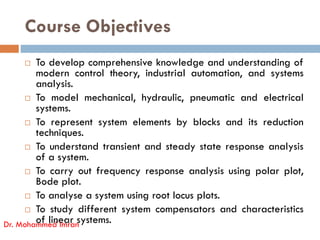
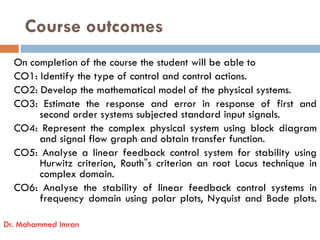
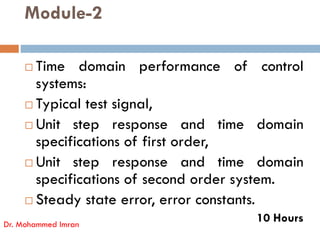
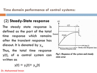
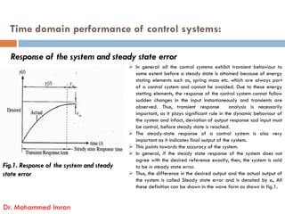
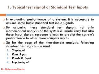
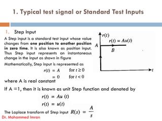
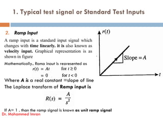
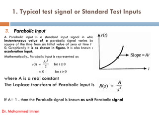
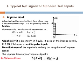
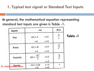
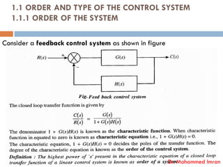
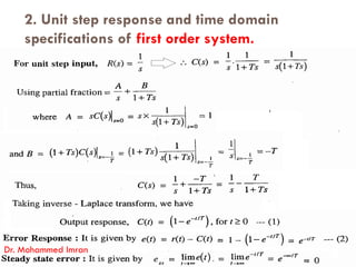
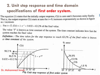
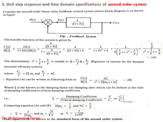
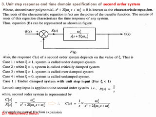
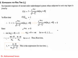
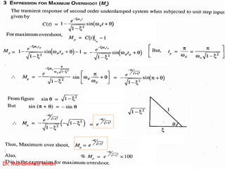
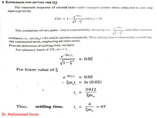
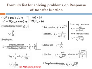
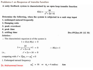
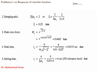
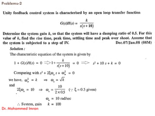
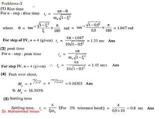
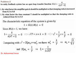
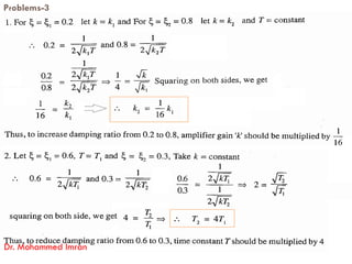
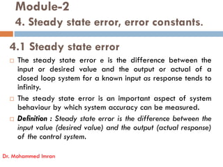
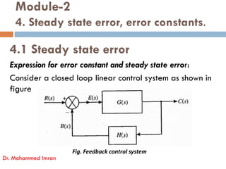
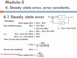
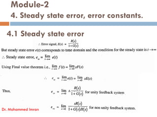
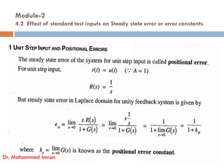
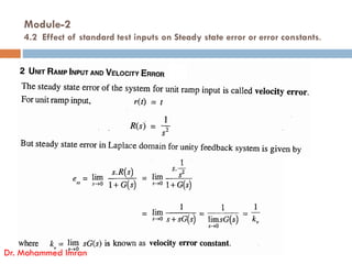
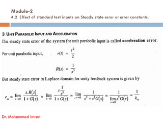
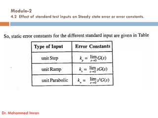

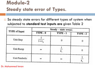

The document outlines a Control Engineering course (code 18ME71) for mechanical engineering students, detailing course objectives, outcomes, and the structure of the syllabus. It covers topics like system modeling, transient and steady-state analysis, frequency response, stability analysis, and various standard test inputs used for evaluating system performance. The course is structured into modules, with specified textbooks and references for further reading.