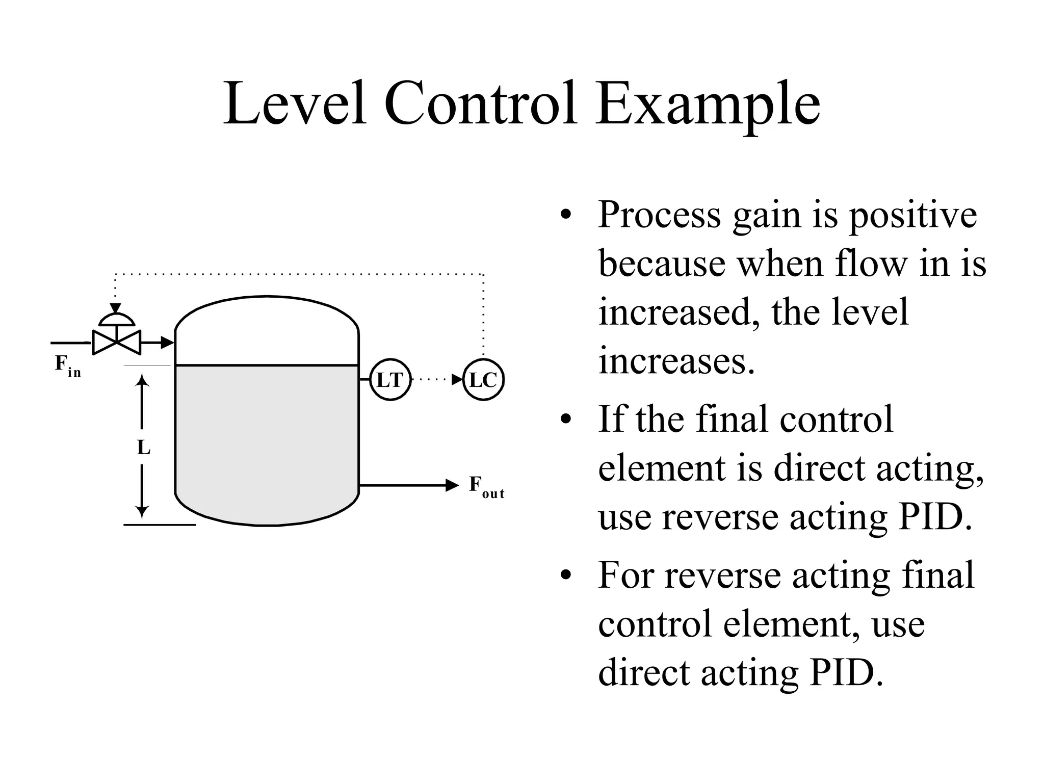
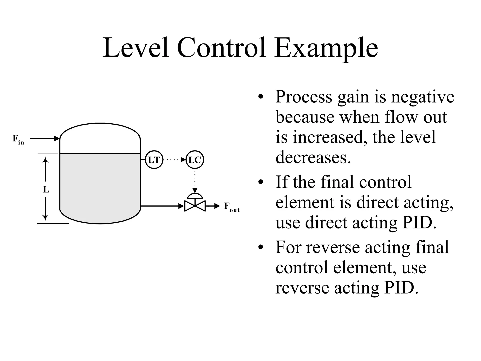
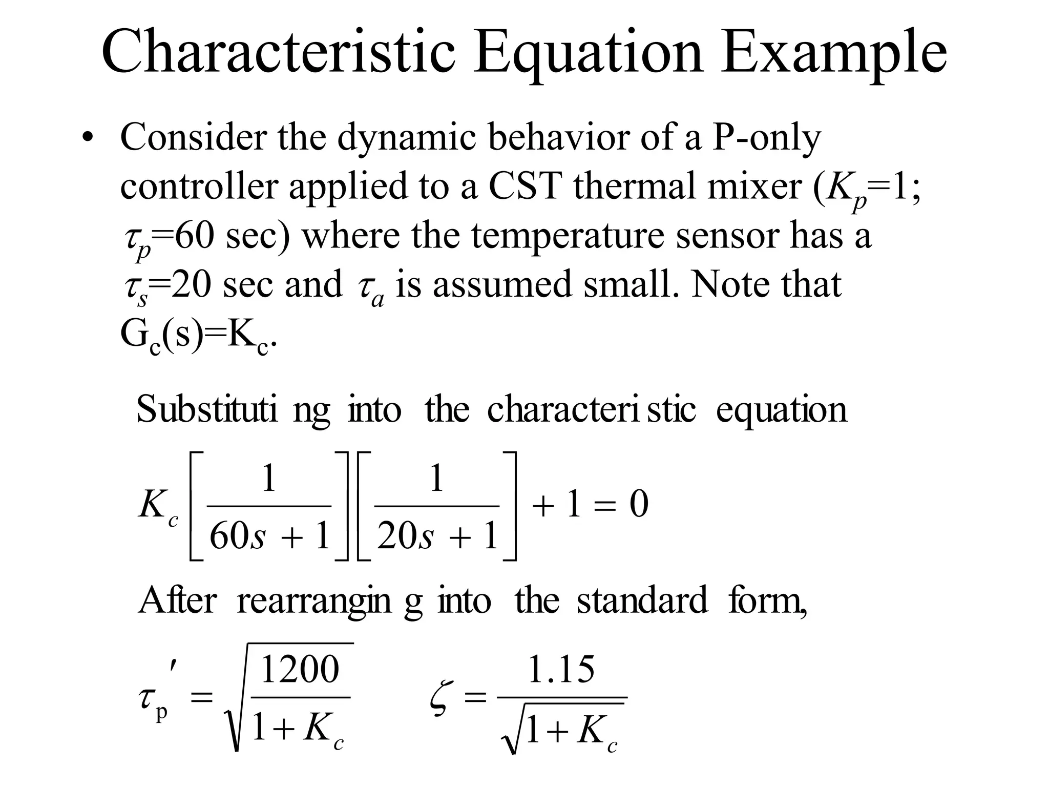
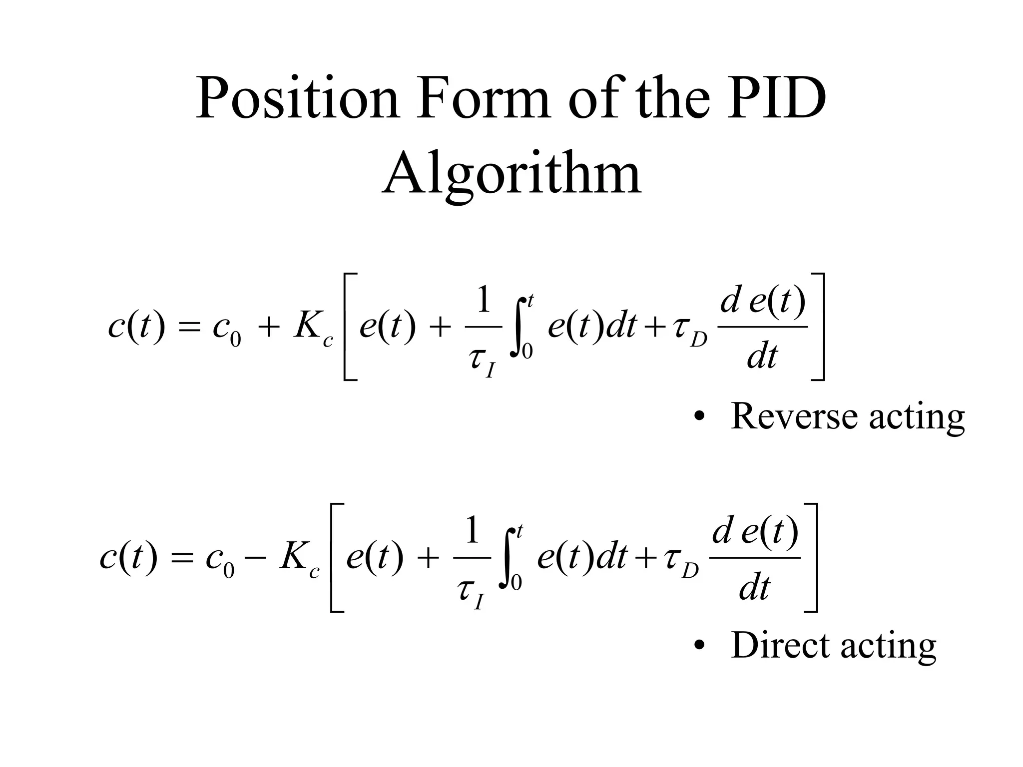
This document discusses PID control. It begins by explaining that PID controllers are the most common type used in process industries. It then provides the general feedback control loop model and shows how to derive the closed-loop transfer functions. Next, it defines the characteristic equation and provides an example using a P-only controller. The document continues by presenting the position and velocity forms of the PID algorithm as well as digital equivalents. It concludes by discussing different PID configurations available in distributed control systems.

1. Chapter 6
PID Control

2. PID Controls
• Most common controller in the CPI.
• Came into use in 1930’s with the
introduction of pneumatic controllers.
• Extremely flexible and powerful control
algorithm when applied properly.

3. General Feedback Control Loop
Ys
(s)
C(s) U(s)
Ysp(s)
Gc(s)
Y(s)
D(s)
Ga(s) Gp(s)
Gs(s)
Gd(s)
E(s)
+-
++

4. Closed Loop Transfer Functions
• From the general feedback control loop and using
the properties of transfer functions, the following
expressions can be derived:
1
)
(
)
(
)
(
)
(
)
(
)
(
)
(
)
(
)
(


s
G
s
G
s
G
s
G
s
G
s
G
s
G
s
Y
s
Y
s
c
a
p
c
a
p
sp
1
)
(
)
(
)
(
)
(
)
(
)
(
)
(


s
G
s
G
s
G
s
G
s
G
s
D
s
Y
s
c
a
p
d

5. Characteristic Equation
• Since setpoint tracking and disturbance rejection
have the same denominator for their closed loop
transfer functions, this indicates that both setpoint
tracking and disturbance rejection have the same
general dynamic behavior.
• The roots of the denominator determine the
dynamic characteristics of the closed loop process.
• The characteristic equation is given by:
0
1
)
(
)
(
)
(
)
( 

s
G
s
G
s
G
s
G s
c
a
p

6. Characteristic Equation Example
• Consider the dynamic behavior of a P-only
controller applied to a CST thermal mixer (Kp=1;
tp=60 sec) where the temperature sensor has a
ts=20 sec and ta is assumed small. Note that
Gc(s)=Kc.
c
c
c
K
K
s
s
K





















1
15
.
1
1
1200
form,
standard
the
into
g
rearrangin
After
0
1
1
20
1
1
60
1
equation
stic
characteri
the
into
ng
Substituti
p 
t

7. Example Continued- Analysis of
the Closed Loop Poles
• When Kc =0, poles are -0.05 and -0.0167
which correspond to the inverse of tp and ts.
• As Kc is increased from zero, the values of
the poles begin to approach one another.
• Critically damped behavior occurs when the
poles are equal.
• Underdamped behavior results when Kc is
increased further due to the imaginary
components in the poles.

8. Position Form of the PID
Algorithm
• Reverse acting
• Direct acting









 
t
D
I
c
dt
t
e
d
dt
t
e
t
e
K
c
t
c
0
0
)
(
)
(
1
)
(
)
( t
t









 
t
D
I
c
dt
t
e
d
dt
t
e
t
e
K
c
t
c
0
0
)
(
)
(
1
)
(
)
( t
t

9. Definition of Terms
• e(t)- the error from setpoint [e(t)=ysp-ys].
• Kc- the controller gain is a tuning parameter
and largely determines the controller
aggressiveness.
• tI- the reset time is a tuning parameter and
determines the amount of integral action.
• tD- the derivative time is a tuning
parameter and determines the amount of
derivative action.

10. Level Control Example
• Process gain is positive
because when flow in is
increased, the level
increases.
• If the final control
element is direct acting,
use reverse acting PID.
• For reverse acting final
control element, use
direct acting PID.
Fout
Fin
L
LC
LT

11. Level Control Example
Fout
Fin
L
LC
LT
• Process gain is negative
because when flow out
is increased, the level
decreases.
• If the final control
element is direct acting,
use direct acting PID.
• For reverse acting final
control element, use
reverse acting PID.

12. Guidelines for Selecting Direct
and Reverse Acting PID’s
• Consider a direct acting final control element
to be positive and reverse to be negative.
• If the sign of the product of the final control
element and the process gain is positive, use
the reverse acting PID algorithm.
• If the sign of the product is negative, use the
direct acting PID algorithm.

13. Proportional Band
c
K
PB
%
100

• Another way to express the controller gain.
• Kc in this formula is dimensionless. That is, the
controller output is scaled 0-100% and the error
from setpoint is scaled 0-100%.
• In more frequent use 10-15 years ago, but it still
appears as an option on DCS’s.

14. Conversion from PB to Kc
• Proportional band is equal to 200%.
• The range of the error from setpoint is 200 psi.
• The controller output range is 0 to 100%.
psi
/
%
25
.
0
psi
200
%
100
5
.
0
5
.
0
%
200
%
100
%
100











c
D
c
K
PB
K

15. Digital Equivalent of PID
Controller
• The trapezoidal
approximation of the
integral.
• Backward difference
approximation of the
first derivative
 





0
1
)
(
)
(
n
i
t
t
i
e
dt
t
e
t
t
t
e
t
e
dt
t
e
d





)
(
)
(
)
(

16. Digital Version of PID Control
Algorithm
t
t
n
t
t
t
e
t
e
t
i
e
t
t
e
K
c
t
c
n
i
D
I
c

















 
1
0
)
(
)
(
)
(
)
(
)
( t
t

17. Derivation of the Velocity Form
of the PID Control Algorithm















 

n
i
D
I
c
t
t
t
e
t
e
t
i
e
t
t
e
K
c
t
c
1
0
)
(
)
(
)
(
)
(
)
( t
t





















 


1
1
0
)
2
(
)
(
)
(
)
(
)
(
n
i
D
I
c
t
t
t
e
t
t
e
t
i
e
t
t
t
e
K
c
t
t
c t
t



























t
t
t
e
t
t
e
t
e
t
e
t
t
t
e
t
e
K
t
c D
I
c
)
2
(
)
(
2
)
(
)
(
)
(
)
(
)
(
______
__________
__________
__________
__________
__________
t
t

18. Velocity Form of PID Controller
• Note the difference in proportional, integral, and
derivative terms from the position form.
• Velocity form is the form implemented on DCSs.
 
 
Controller
Acting
Direct
)
(
)
(
)
(
Controller
Acting
Reverse
)
(
)
(
)
(
)
2
(
)
(
2
)
(
)
(
)
(
)
(
)
(
t
c
t
t
c
t
c
t
c
t
t
c
t
c
t
t
t
e
t
t
e
t
e
t
e
t
t
t
e
t
e
K
t
c D
I
c




































 t
t

19. Correction for Derivative Kick
• Derivative kick occurs when a setpoint change is
applied that causes a spike in the derivative of the
error from setpoint.
• Derivative kick can be eliminated by replacing the
approximation of the derivative based on the error
from setpoint with the negative of the approximation
of the derivative based on the measured value of the
controlled variable, i.e.,
t
t
t
y
t
t
y
t
y s
s
s
D








)
2
(
)
(
2
)
(
t

20. Correction for Aggressive
Setpoint Tracking
• For certain process, tuning the controller for good
disturbance rejection performance results in
excessively aggressive action for setpoint changes.
• This problem can be corrected by removing the
setpoint from the proportional term. Then setpoint
tracking is accomplished by integral action only.
   
)
(
)
(
by
for
d
substitute
)
(
)
( t
y
t
t
y
K
t
t
e
t
e
K s
s
c
c 






21. The Three Versions of the PID
Algorithm Offered on DCS’s
• (1) The original form in which the
proportional, integral, and derivative terms
are based on the error from setpoint



























t
t
t
e
t
t
e
t
e
t
e
t
t
t
e
t
e
K
t
c D
I
c
)
2
(
)
(
2
)
(
)
(
)
(
)
(
)
( t
t

22. The Three Versions of the PID
Algorithm Offered on DCSs
• (2) The form in which the proportional and
integral terms are based on the error from
setpoint while the derivative-on-
measurement is used for the derivative term.



























t
t
t
y
t
t
y
t
y
t
e
t
t
t
e
t
e
K
t
c s
s
s
D
I
c
)
2
(
)
(
2
)
(
)
(
)
(
)
(
)
( t
t

23. The Three Versions of the PID
Algorithm Offered on DCS’s
• (3) The form in which the proportional and
derivative terms are based on the process
measurement and the integral is based on
the error from setpoint.



























t
t
t
y
t
t
y
t
y
t
e
t
t
y
t
t
y
K
t
c s
s
s
D
I
s
s
c
)
2
(
)
(
2
)
(
)
(
)
(
)
(
)
( t
t

24. Laplace Transform for a PID
Controller









 s
s
K
s
E
s
C
s
G D
I
c
c t
t
1
1
)
(
)
(
)
(

25. Example for a First Order
Process with a PI Controller
5
.
1
5
0
1
15
25
g
Rearrangin
0
1
10
2
2
1
5
1
:
Equation
stic
Characteri
5
1
10
2
2



























t
t
t
p
p
p
I
c
s
s
s
s
K
K

26. Example of a PI Controller Applied
to a Second Order Process
08
.
0
and
37
.
4
with
response
order
second
a
and
764
.
0
0
1
2
20
25
g
Rearrangin
0
1
1
1
1
20
25
1
:
Equation
stic
Characteri
2
;
5
;
1
;
1
;
1
1
2
3
2































t

t
t
p
p
p
I
c
p
s
s
s
s
s
s
K
K

27. Filtering the Process
Measurement
)
(
)
1
(
)
(
)
( t
t
y
f
t
y
f
t
y f
s
f 




• Filtering reduces the effect of sensor noise
by approximating a running average.
• Filtering adds lag when the filtered
measurement is used for control.
• Normally, use the minimum amount of
filtering necessary.
• f- filter factor (0-1)

28. Feedback Loop with Sensor
Filtering
Ys
(s)
C(s) U(s)
Ysp(s)
Gc(s)
Y(s)
D(s)
Ga(s) Gp(s)
Gs(s)
Gd(s)
E(s)
+-
++
Gf(s)
Yf
(s)

29. Effect of Filtering on Closed
Loop Dynamics
)
1
(
2
1
0
1
1
1
1
:
filtering
sensor
with
process
order
first
on
controller
only
P
for
equation
stic
Characteri



























p
c
f
p
f
p
p
c
f
p
p
f
p
p
c
K
K
K
K
s
s
K
K
t
t
t
t

t
t
t
t
t

30. Analysis of Example
• tf is equal to t (1/f-1) as f becomes
small, tf becomes large.
• When tf is small compared to tp, as tf is
increased,  will decrease.
• When tf is large compared to tp, as tf is
increased,  will increase.
• Critical issue is relative magnitude of tf
compare to tp.

31. Effect of the Amount of Filtering
on the Open Loop Response
0 20 40 60 80 100
Time (seconds)
Filtered
Temperature
f=0.2
f=0.1
f=0.3

32. Effect of a Noisy Sensor on
Controlled Variable without Filtering
Time
Manipulated Variable
Product Temperature

33. Effect of a Noisy Sensor on
Controlled Variable with Filtering
Time
Manipulated Variable
Product Temperature

34. An Example of Too Much and
Too Little Filtering
100
102
104
0 50 100 150 200
Time (seconds)
Temperature
(ºC)
f=0.2
f=0.5
f=0.01

35. Properties of Proportional Action
1
1
1
)
(
)
(
)
(
)
( 0






s
K
K
K
K
K
K
s
Y
s
Y
t
e
K
c
t
c
p
c
p
p
c
p
c
sp
c
t
• Closed loop transfer function
base on a P-only controller
applied to a first order process.
• Properties of P control
– Does not change order of process
– Closed loop time constant is
smaller than open loop tp
– Does not eliminate offset.

36. Offset Resulting from P-only
Control
Time
Setpoint
1.0
1
2
3
0
Offset

37. Proportional Action for the
Response of a PI Controller
Time
ys
ysp
cprop

38. Properties of Integral Action
• Based on applying an I-
only controller to a first
order process
• Properties of I control
– Offset is eliminated
– Increases the order by 1
– As integral action is
increased, the process
becomes faster, but at the
expense of more sustained
oscillations
p
c
p
I
p
c
p
I
I
p
c
I
p
c
p
I
sp
t
I
c
K
K
K
K
s
K
K
s
K
K
s
Y
s
Y
dt
t
e
K
c
t
c
t
t

t
t
t
t
t
t
t
2
1
1
1
)
(
)
(
)
(
)
(
2
0
0







 

39. Integral Action for the Response
of a PI Controller
Time
ys
ysp
cint

40. Properties of Derivative Action
• Closed loop transfer function for derivative-only
control applied to a second order process.
• Properties of derivative control:
– Does not change the order of the process
– Does not eliminate offset
– Reduces the oscillatory nature of the
feedback response
  1
2
)
(
)
(
)
(
)
(
2
2
0






s
K
K
s
s
K
K
s
Y
s
Y
dt
t
de
K
c
t
c
D
p
c
p
p
D
p
c
sp
D
c
t
t
t
t
t

41. Derivative Action for the
Response of a PID Controller
Time
ys
ysp
cder

42. PID Controller Design Issues
• Over 90% of control loops use PI controller.
• P-only: used for fast responding processes
that do not require offset free operation
(e.g., certain level and pressure controllers)
• PI: used for fast responding processes that
require offset free operation (e.g., certain
flow, level, pressure, temperature, and
composition controllers)

43. PID Controller Design Issues
• PID: use for sluggish processes (i.e., a process
with large deadtime to time constant ratios) or
processes that exhibit severe ringing for PI
controllers. PID controllers are applied to
certain temperature and composition control
loops. Use derivative action when:
1

p
p
t


44. Comparison between PI and PID
for a Low p/tp Ratio
Time
PI
PID

45. Comparison between PI and PID
for a High p/tp Ratio
Time
PID
PI

46. Analysis of Several Commonly
Encountered Control Loops
• Flow control loops
• Level control loops
• Pressure control loops
• Temperature control loops
• Composition control loops

47. Flow Control Loop
FT
FC Flow
Setpoint
• Since the flow sensor and the process are so fast,
the dynamics of the flow control loop is controlled
by the dynamics of the control valve.
• Almost always use PI controller.

48. Deadband of a Control Valve
Time
Stem Position
Air Pressure
• Deadband of industrial valves is between ±10%-
±25%.
• As a result, small changes in the air pressure
applied to the valve do not change the flow rate.

49. Deadband of Flow Control Loop
0 20 40 60
Time (seconds)
Flow
Rate
• A control valve (deadband of ±10-25%) in a flow
control loop or with a positioner typically has a
deadband for the average flow rate of less than
±0.5% due to the high frequency opening and
closing of the valve around the specified flow rate.

50. Level Control Loop
Fin
FC
LT
RSP
FT
Fout
Lsp
LC
• Dynamics of the sensor
and actuator are fast
compared to the
process.
• If operators want
control to setpoint, use
PI controller with small
amount of integral
action, otherwise use P-
only controller.

51. Pressure Control Process
PT
PC
Vent
Psp
C.W.
• The process and the sensor are generally faster
than the actuator.
• Use P-only controller unless offset elimination is
important then use a PI controller.

52. Temperature Control Loop
RSP
TT
FC
Gas
FT
TC Tsp
Process
Stream
• The dynamics of the
process and sensor are
usually slower than
the actuator.
• Use a PI controller
unless the process is
sufficiently sluggish to
warrant a PID
controller.

53. Analysis of PI Controller Applied
to Typical Temperature Loop
14
.
0
28
057
.
0
50
.
1
37
.
0
48
051
.
0
80
.
0
74
.
0
140
056
.
0
10
.
0
48
.
1
325
057
.
0
02
.
0
ζ
τ
0
1
1
20
1
1
60
30
1
1
20
;
60
;
30



























p
1
p
c p
K
K
s
s
K
s
K
p
c
v
p
I t
t
t

54. Further Analysis of Dynamic of a
Typical Temperature Control Loop
• Note that as the controller gain is increased,
i.e., KcKp increase, the closed loop time
constant becomes smaller.
• Also, note that as the controller gain is
increased, the value of  decreases.

55. Composition Control Loop
C.W.
AT
FT
FC
AC
RSP
• The process is usually
the slowest element
followed by the sensor
with the actuator being
the fastest.
• Use a PI controller
unless the process is
sufficiently sluggish to
warrant a PID
controller.

56. Overview
• The characteristic equation determines the
dynamic behavior of a closed loop system
• There are a number of different ways to apply a
PID controller.
• Proportional, integral, and derivative action each
have unique characteristics.
• Use a PI controller unless offset is not important
or if the process is sluggish.
• When analyzing the dynamics of a loop, consider
the dynamics of the actuator, the process, and the
sensor separately.