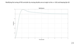
This document discusses different types of PID controllers including proportional (P), integral (I), derivative (D), PI, PD, and PID controllers. It provides the transfer functions and describes the basic functionality of each type. Tuning methods for PID controllers are presented, including Ziegler-Nichols tuning when the dynamic plant model is known or unknown. Examples are given to illustrate tuning a PID controller to achieve approximately 25% overshoot for a control system.

1. PID Controllers
1

2. Transfer Function
2
Proportional Gain
Derivative Time Integral Time
𝐶 𝑠 = 𝐾 𝑃 1 + 𝑇𝑑 𝑠 +
1
𝑇𝑖 𝑠

3. 3
Problem 1.1- For the system shown in Fig. 1.1 draw the open loop step response.
1
𝑠2 + 10𝑠 + 20
Fig. 1.1
input output
Solution- with the help of following command in MATLAB response is obtained.
G= tf(1,[1 10 20]);
step(G);

4. 4
without any controller

5. Proportional Control (P)
 Easy Tuning
 Introduce steady state error called offset.
5
Controller Process
error
Reference
Input output+
-
r(t) u(t)e(t)
feedback

6. 6
For problem 1.1 using a P controller with Kp=500 and for unity feedback.

7. Integral Control (I)
 No steady state error (for step input).
 Slow response.
7

8. 8
For problem 1.1 using a I controller with Ki=70 and for unity feedback.

9. Derivative Control (D)
can not respond to sudden error.
9

10. PI Controller
 No offset associate with P controller.
 Fast response.
 for sinusoidal input phase of the controller output legs by ,
hence it is similar to Leg Compensator.
10
tan−1
1
𝑇𝑖 𝜔

11. 11
For problem 1.1 using a PI controller with Kp=30 & Ki=70 and for unity feedback.

12. PD Controller
 used for system having large no of time constant.
 for sinusoidal input phase of the controller output lead by
hence it is similar to Lead Compensator.
12
tan−1
𝜔𝑇𝑑

13. 13
For problem 1.1 using a PD controller with Kp=500 & Kd=10 and for unity feedback.

14. PID Controller
 Tuning is difficult
 Used for controlling slow variables.
14

15. 15
For problem 1.1 using a PID controller with Kp=500, Ki=400 & Kd=50 and for unity
feedback.

16. Performance of Different Controllers
Parameter PI PD PID
Rise Time
Band Width
Stability
Damping Ratio
Peak Overshoot
16

17. Tuning of PID Controller
17

18. Tuning Methods
1. Dynamic Model of the plant is Not known
I. The Step Response of the plant is S-shaved Curve
II. The Step Response of the plant is not S-shaved Curve
2. Dynamic Model of the plant is known
I. The plant has no integral term in the transfer function
II. The plant has an integral term in the transfer function
18

19. 19
1. Dynamic Model of the plant is Not known
I. The Step Response of the plant is S-shaved
CurveZiegler- Nichols Method
 Open Loop response for a step input is
determined
 The values can be calculated as:
Controller KP Ti Td
P T/L 0
PI 0.9(T/L) L/0.3 0
PID 1.2(T/L) 2L 0.5L

20. 20
1. Dynamic Model of the plant is Not known
II. The Step Response of the plant is not S-shaved
Curve
No specific tuning method available.

21. 21
2. Dynamic Model of the plant is known
I. The plant has no integral term in the
transfer function
Ziegler- Nichols Method
 First P mode is selected by putting Td=0 and Ti= ∞
(infinity).
 Increase KP from 0 to critical value Kcr such that
system exhibits sustained oscillations with time
period Pcr.
Controller KP Ti Td
P 0.5Kcr 0
PI 0.45Kcr Pcr/1.2
PID 0.6Kcr Pcr/2 Pcr/8

22. 22
Problem 1.2: Consider the control system shown in Fig. 1.2 which has a PID controller to
control the system.
Fig. 1.2
Then obtain a unit step response curve and check if the designed system exhibits
approximately 25% maximum overshoot. If the maximum is 40% or more, then make a fine
tuning of PID controller to reduce the maximum overshoot to approximately 25% or less.

23. 23
By applying Ziegler- Nichols Method response is shown in fig which have peak overshoot about 60%, hence fine
tuning of PID controller is further needed.

24. 24
Modifying the tuning of PID controller by moving double zero at origin to the s= -0.65 and keeping Kp=18

25. 25
2. Dynamic Model of the plant is known
II. The plant has an integral term in the
transfer function
 Initially low value of p-control and Td =0 &
Ti = ∞ (infinity).
 KP Is increased slowly till P2/P1 is 0.25. then
value is given as:
KP =gain when P2/P1 is 0.25
Ti = td/6
Td = td/1.5