Paper id 21201482

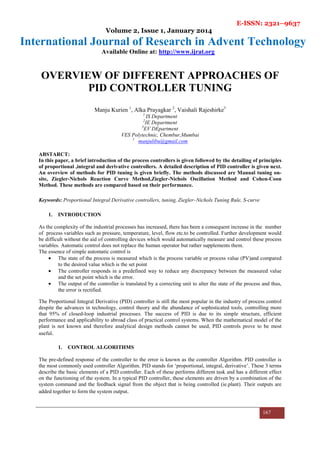
E-ISSN: 2321–9637
Volume 2, Issue 1, January 2014
International Journal of Research in Advent Technology
Available Online at: http://www.ijrat.org
167
OVERVIEW OF DIFFERENT APPROACHES OF
PID CONTROLLER TUNING
Manju Kurien 1
, Alka Prayagkar 2
, Vaishali Rajeshirke3
1
IS Department
2
IE Department
3
EV DEpartment
VES Polytechnic, Chembur,Mumbai
1
manjulibu@gmail.com
ABSTARCT:
In this paper, a brief introduction of the process controllers is given followed by the detailing of principles
of proportional ,integral and derivative controllers. A detailed description of PID controller is given next.
An overview of methods for PID tuning is given briefly. The methods discussed are Manual tuning on-
site, Ziegler-Nichols Reaction Curve Method,Ziegler-Nichols Oscillation Method and Cohen-Coon
Method. These methods are compared based on their performance.
Keywords: Proportional Integral Derivative controllers, tuning, Ziegler–Nichols Tuning Rule, S-curve
1. INTRODUCTION
As the complexity of the industrial processes has increased, there has been a consequent increase in the number
of process variables such as pressure, temperature, level, flow etc.to be controlled. Further development would
be difficult without the aid of controlling devices which would automatically measure and control these process
variables. Automatic control does not replace the human operator but rather supplements them.
The essence of simple automatic control is
• The state of the process is measured which is the process variable or process value (PV)and compared
to the desired value which is the set point
• The controller responds in a predefined way to reduce any discrepancy between the measured value
and the set point which is the error.
• The output of the controller is translated by a correcting unit to alter the state of the process and thus,
the error is rectified.
The Proportional Integral Derivative (PID) controller is still the most popular in the industry of process control
despite the advances in technology, control theory and the abundance of sophisticated tools, controlling more
that 95% of closed-loop industrial processes. The success of PID is due to its simple structure, efficient
performance and applicability to abroad class of practical control systems. When the mathematical model of the
plant is not known and therefore analytical design methods cannot be used, PID controls prove to be most
useful.
1. CONTROL ALGORITHMS
The pre-defined response of the controller to the error is known as the controller Algorithm. PID controller is
the most commonly used controller Algorithm. PID stands for ‘proportional, integral, derivative’. These 3 terms
describe the basic elements of a PID controller. Each of these performs different task and has a different effect
on the functioning of the system. In a typical PID controller, these elements are driven by a combination of the
system command and the feedback signal from the object that is being controlled (ie.plant). Their outputs are
added together to form the system output.

E-ISSN: 2321–9637
168
2.1. The proportional Controller
The proportional term produces an output value that is proportional to the current error value. The proportional
response can be adjusted by multiplying the error by a constant Kp, called the proportional gain constant. If the
proportional gain is too high, the system can become unstable. If the proportional gain is too low, the control
action may be too small when responding to system disturbances. Tuning theory and industrial practice indicate
that the proportional term should contribute the bulk of the output change.
The proportional term is given by:
Fig 1: The response of proportional Controller
2.1.1. Offset
Offset, also called droop, is deviation that remains after a process has stabilized. Offset is an inherent
characteristic of the proportional mode of control. In other words, the proportional mode of control will not
necessarily return a controlled variable to its set point. Droop may be mitigated by adding a compensating bias
term (setting the set point above the true desired value), or corrected by adding an integral term.
2.2. The Integral Controller
The integral in a PID controller is the sum of the instantaneous error over time and gives the accumulated offset
that should have been corrected previously. The accumulated error is then multiplied by the integral gain and
added to the controller output. The integral term accelerates the movement of the process towards set point and
eliminates the residual steady-state error that occurs with a pure proportional controller. However, since the
integral term responds to accumulated errors from the past, it can cause the present value to overshoot the set
point value.
The integral term is given by:

E-ISSN: 2321–9637
169
Fig 2: The response of integral Controller
2.3. The Derivative Controller
Derivative control is used to reduce the magnitude of the overshoot produced by the integral component and
improve the combined controller-process stability. However, the derivative term slows the transient response of
the controller.
The derivative term is given by:
Fig 3: The response of derivative Controller

E-ISSN: 2321–9637
170
2. PID CONTROLLERS
A PID controller calculates an "error" value as the difference between a measured process variable and a desired
set point. The controller attempts to minimize the error by adjusting the process control inputs.
Defining u(t) as the controller output, the final form of the PID algorithm is:
where
Kp: Proportional gain, a tuning parameter
Ki: Integral gain, a tuning parameter
Kd: Derivative gain, a tuning parameter
e: Error = SP − PV
t: Time or instantaneous time (the present)
3.1 Laplace form of the PID controller
PID controller in Laplace transform form:
Having the PID controller written in Laplace form and having the transfer function of the controlled system
makes it easy to determine the closed-loop transfer function of the system.
3.2 PID Pole Zero Cancellation
The PID equation can be written in this following form:
When this form is used it is easy to determine the closed loop transfer function.
If, , then,
This can be very useful to remove unstable poles.

E-ISSN: 2321–9637
171
3. PID CONTROLLER TUNING
Tuning a control loop is the adjustment of its control parameters (gain/proportional band, integral gain/reset,
derivative gain/rate) to the optimum values for the desired control response. Stability (bounded oscillation) is a
basic requirement, but beyond that, different systems have different behaviour, different applications have
different requirements, and requirements may conflict with each.
Each of the three mathematical control functions in PID- Proportional, Integral &Derivative is governed by a
user-defined parameter. These parameters need to be adjusted to optimize the precision of control. The process
of determining the values of these parameters is known as PID Tuning. The goal of good tuning is to have the
fastest response possible without causing instability.
Designing and tuning a PID controller appears to be conceptually intuitive, but can be hard in practice, if
multiple (and often conflicting) objectives such as short transient and high stability are to be achieved. Usually,
initial designs obtained by all means need to be adjusted repeatedly through computer simulations until the
closed-loop system performs or compromises as desired.
Some processes have a degree of non-linearity and so parameters that work well at full-load conditions don't
work when the process is starting up from no-load; this can be corrected by gain scheduling (using different
parameters in different operating regions). PID controllers often provide acceptable control using default
tunings, but performance can generally be improved by careful tuning, and performance may be unacceptable
with poor tuning.
There are several methods for tuning a PID loop. The most effective methods generally involve the development
of some form of process model, then choosing P, I, and D based on the dynamic model parameters. Manual
tuning methods can be relatively inefficient, particularly if the loops have response times on the order of
minutes or longer.
The choice of method will depend largely on whether or not the loop can be taken "offline" for tuning, and the
response time of the system. If the system can be taken offline, the best tuning method often involves subjecting
the system to a step change in input, measuring the output as a function of time, and using this response to
determine the control parameters.
Commonly used methods of tuning rules :
Manual tuning on-site
Ziegler-Nichols Reaction Curve Method
Ziegler-Nichols Oscillation Method
Cohen-Coon Method
4.1 Manual tuning
If the system must remain online, one tuning method is to first set integral constant Ki and derivative constant
Kd values to zero. Increase the proportional constant Kp until the output of the loop oscillates, then the Kp should
be set to approximately half of that value for a "quarter amplitude decay" type response. Then increase Ki until
any offset is corrected in sufficient time for the process. However, too much Ki will cause instability. Finally,
increase Kd, if required, until the loop is acceptably quick to reach its reference after a load disturbance.
However, too much Kd will cause excessive response and overshoot. A fast PID loop tuning usually overshoots
slightly to reach the setpoint more quickly; however, some systems cannot accept overshoot, in which case an
over-damped closed-loop system is required, which will require a Kp setting significantly less than half that of
the Kp setting causing oscillation.
Table1: Effects of increasing a parameter independently
Parameter Rise time Overshoot Settling time Steady-state error Stability
Kp Decrease Increase Small change Decrease Degrade
Ki Decrease Increase Increase Decrease significantly Degrade
Kd Minor decrease Minor decrease Minor decrease No effect in theory Improve if Kd small

E-ISSN: 2321–9637
172
4.2 Ziegler–Nichols tuning method
The most commonly used method is Ziegler–Nichols. In order to understand this method, the relationship of the
constants Kp,KI and KD with the 4 major characteristic of the closed loop responses such as rise time, settling
time, overshoot and steady state error of the system should be analyzed. This is shown below:
Table2: The relationship of the constants Kp,KI and KD with characteristic of the closed loop responses
Response Rise Time Overshoot Settling Time S-S Error
Kp Decrease Increase NT Decrease
KI Decrease Increase Increase Eliminate
KD NT Decrease Decrease NT
NT:No definite trend. Minor change
Typical steps for designing a PID controller are:
• Determine what characteristicsnof the system needs to be improved
• Use Kp to decrease the rise time
• Use KD to reduce the overshoot and settling time
• Use KI to eliminate steady state error.
This works in many cases,but to have a good starting point, a good set of initial parameters need to be found out
easily and quickly. It can be done with Ziegler-Nichols tuning rule. Ziegler and Nichols proposed rules for
determining values of the proportional gain Kp, integral time Ti, and derivative time Td based on the transient
response characteristics of a given plant. Such determination of the parameters of PID controllers or tuning of
PID controllers can be made by engineers on-site by experiments on the plant. Such rules suggest a set of values
of Kp, Ti, and Td that will give a stable operation of the system. However, the resulting system may exhibit a
large maximum overshoot in the step response, which is unacceptable. Series of fine tunings are needed until an
acceptable result is obtained.
4.3.1 Ziegler-Nichols Reaction Curve Method (for open loop system)
The Ziegler–Nichols tuning method is a heuristic method of tuning a PID controller, that attempts to produce
good values for the three PID gain parameters. Most PID tuning rules are based on the assumption that the plant
can be approximated by a first-order plus time delay system whose unit-step response resemble an S-shaped
curve with no overshoot. The step response is termed as the Process Reaction Curve in process. This method
applies to plants with neither integrators nor dominant complex-conjugate poles, whose unit-step response
resemble an S-shaped curve with no overshoot. This S-shaped curve is called the reaction curve. Such step
response curves can be generated experimentally or from a dynamic simulation of the plant.
The S-shaped reaction curve can be characterized by two constants, delay time L and time constant T, which are
determined by drawing a tangent line at the inflection point of the curve and finding the intersections of the
tangent line with the time axis and the steady state level line.
For a system, if we assume the system can keep the maximum response speed all the time, then the system will
take exact the time of the time constant to reach its steady-state.
Therefore, the time constant can be identified by taking the maximum slope and measuring the time period
between the points where the maximum slope line crosses the initial and final response lines.

E-ISSN: 2321–9637
173
Fig 4: Reaction curve
Transfer Function:
Table3: Ziegler–Nichols Tuning Rule Based on Step Response of Plant
4.3.2 Ziegler-Nichols Oscillation Method (for closed loop system)
This procedure is carried out through the following steps:
Set the true plant under proportional control, with a very small gain.
Increase the gain until the loop starts oscillating.
Note that linear oscillation is required and that it should be detected at the controller output.
Set Ti = ∞ and Td = 0 using the proportional control action only (see Figure below).

E-ISSN: 2321–9637
174
Fig 5: Closed loop system with proportional controller
Increase Kp from 0 to a critical value Kcr at which the output first exhibits sustained oscillations.
Fig 6: Sustained oscillation with period Pcr. (Pcr is measured in sec.)
Ziegler and Nichols suggested that the values of the parameters Kp , Ti, and Td should be set according to the
formula shown in Table below:
Table 4: Ziegler–Nichols Tuning Rule Based on Critical Gain Kcr and Critical Period Pcr
4.3 Cohen-Coon Reaction Curve Method
Cohen and Coon carried out further studies to find controller settings which, based on the same model, lead to a
weaker dependence on the ratio of delay to time constant.

E-ISSN: 2321–9637
175
Table 5: Comparison of different tuning methods
Method Advantages Disadvantages
Manual Tuning Online method.
Requires experienced personnel.
No math required
Ziegler–Nichols Proven Method. Online method.
Process upset, some trial-and-error,
very aggressive tuning. Used only
for process control systems.
Software Tools
Consistent tuning. Online or offline
method. May include valve and
sensor analysis. Allow simulation
before downloading. Can support
Non-Steady State (NSS) Tuning.
Some cost and training involved.
Cohen-Coon Good process models.
Offline method. Only good for
first-order processes.
Acknowledgments
The authors would like to gratefully acknowledge the help of the college authorities during the preparation
of this manuscript.
References
[1] www.auma.com
[2] www.google.co.in/picturesofPID
[3] www.eetindia.com
[4] PID controller tuning: a short tutorial by JinghuaZhong.
[5] Modern control engineering by K.Ogata
[6] K.j.Astrom,R.M.Murray; Feedback system-an introduction for scientists and engineers
[7] www.mathworks.com

Paper id 21201482

More Related Content

What's hot

Viewers also liked

Similar to Paper id 21201482

More from IJRAT

Paper id 21201482