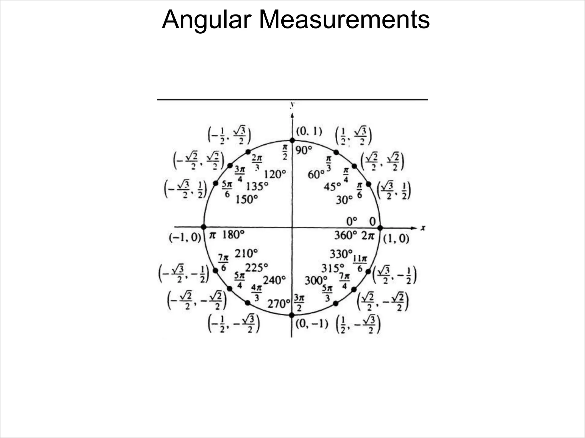
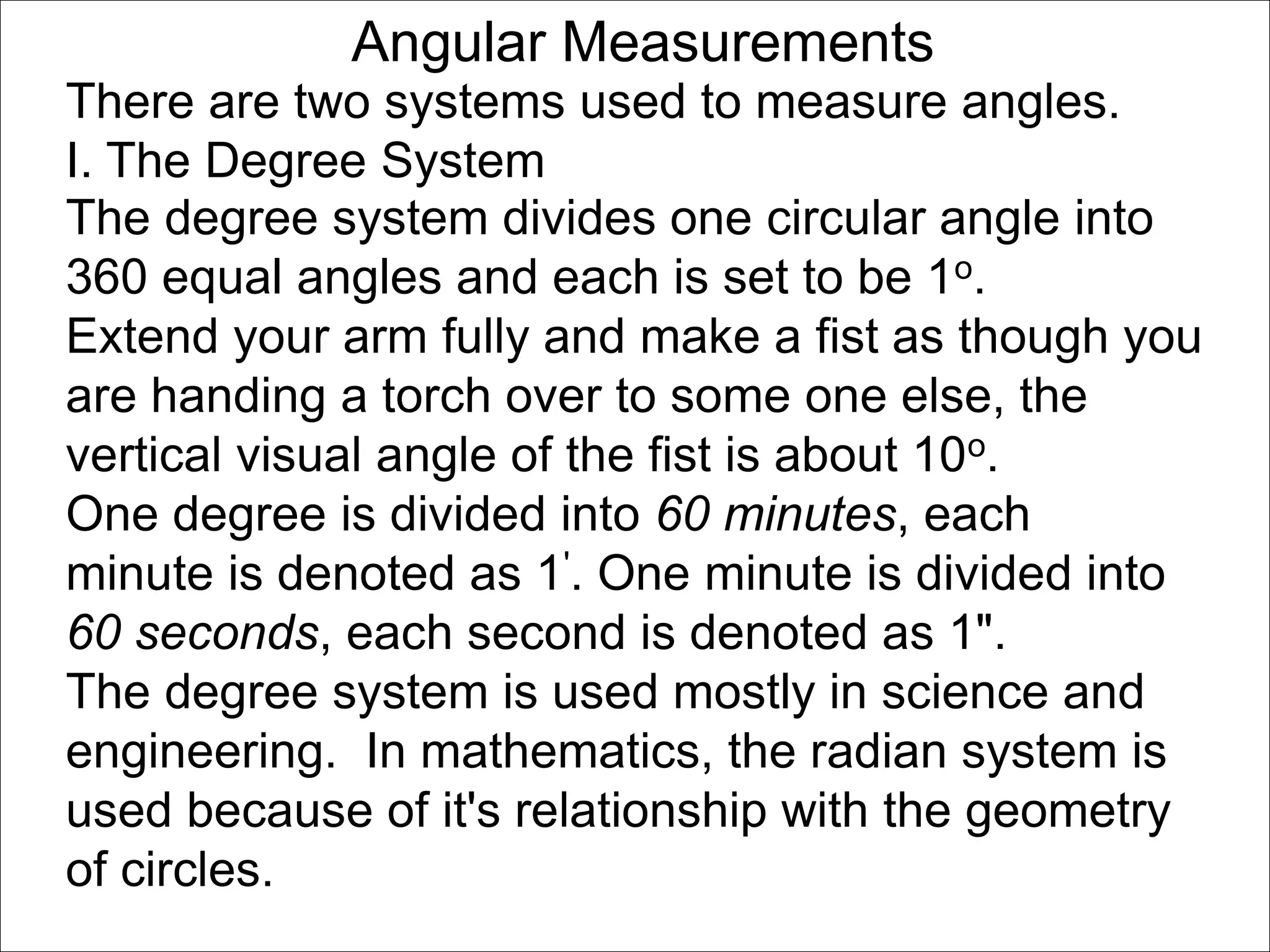
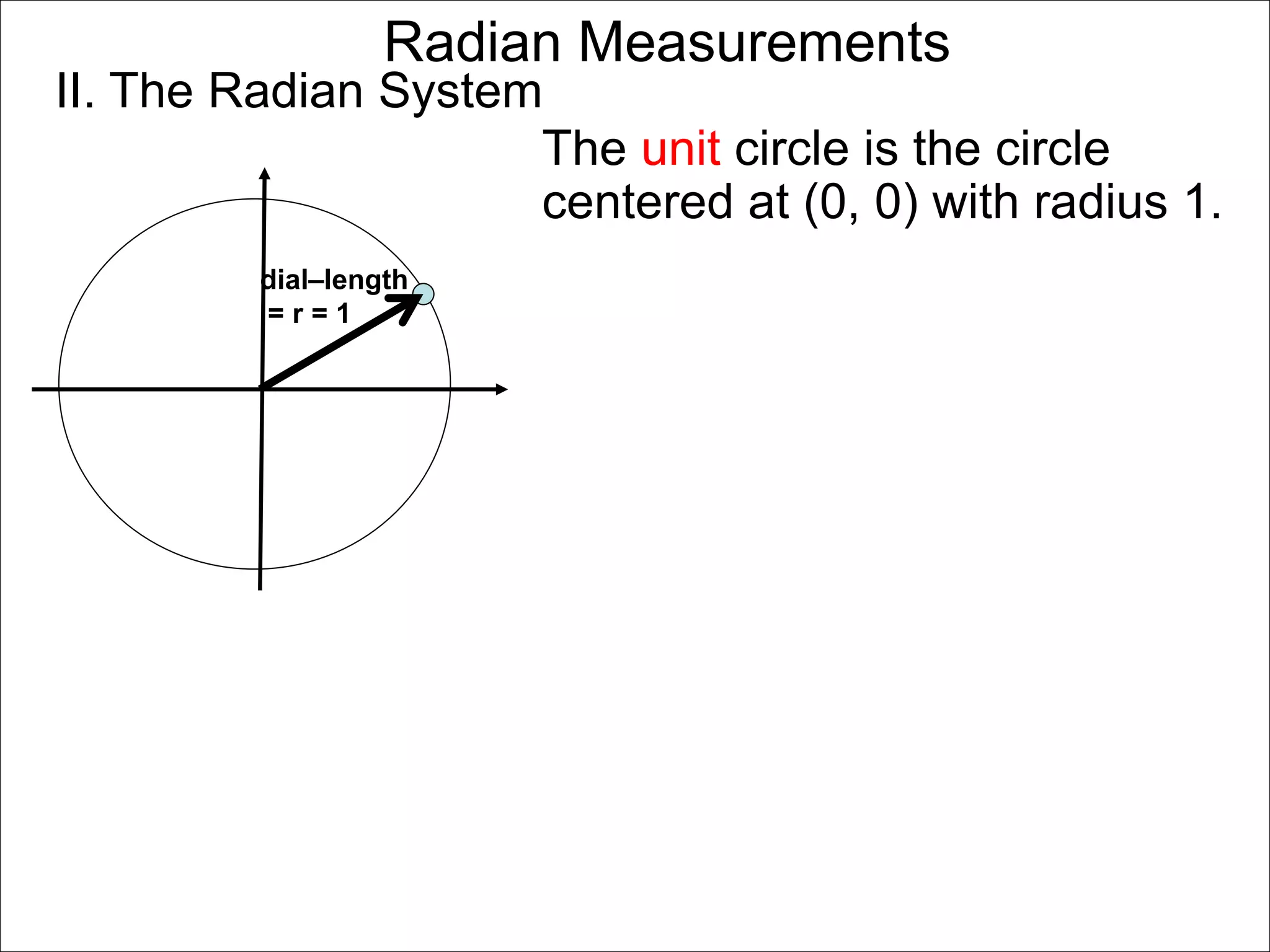
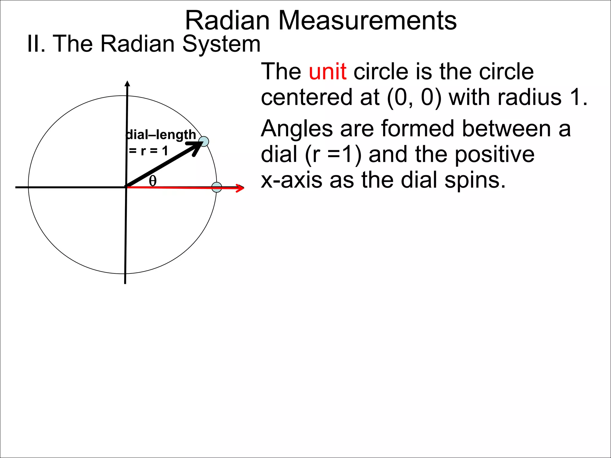
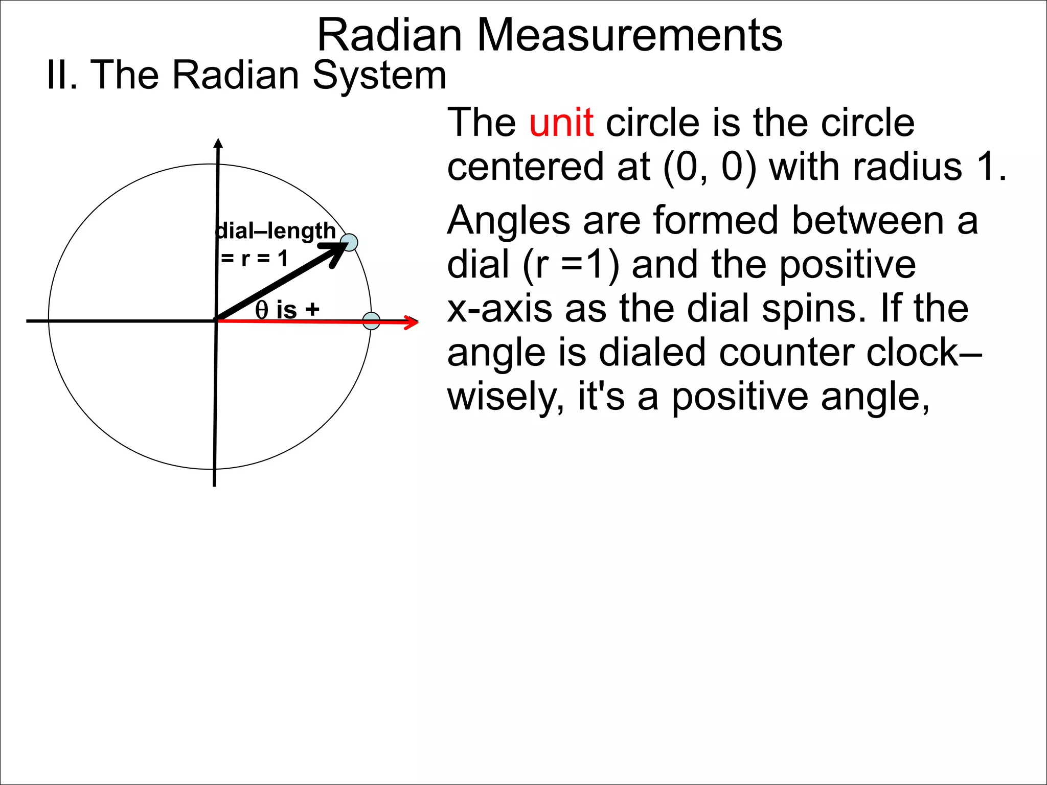
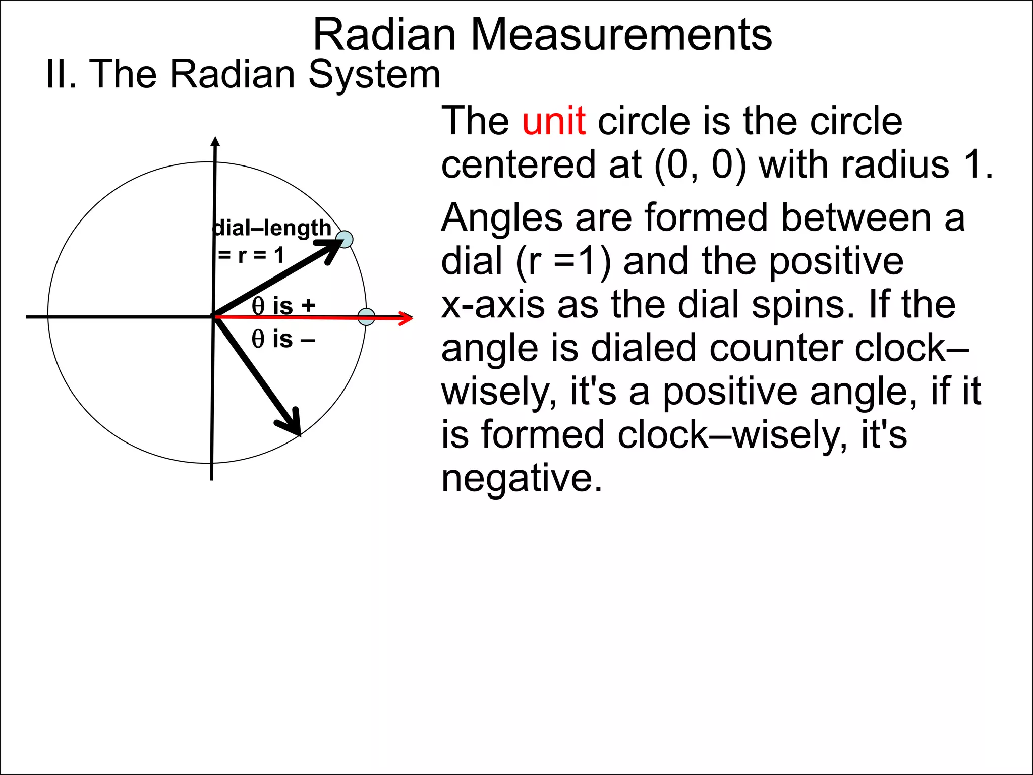
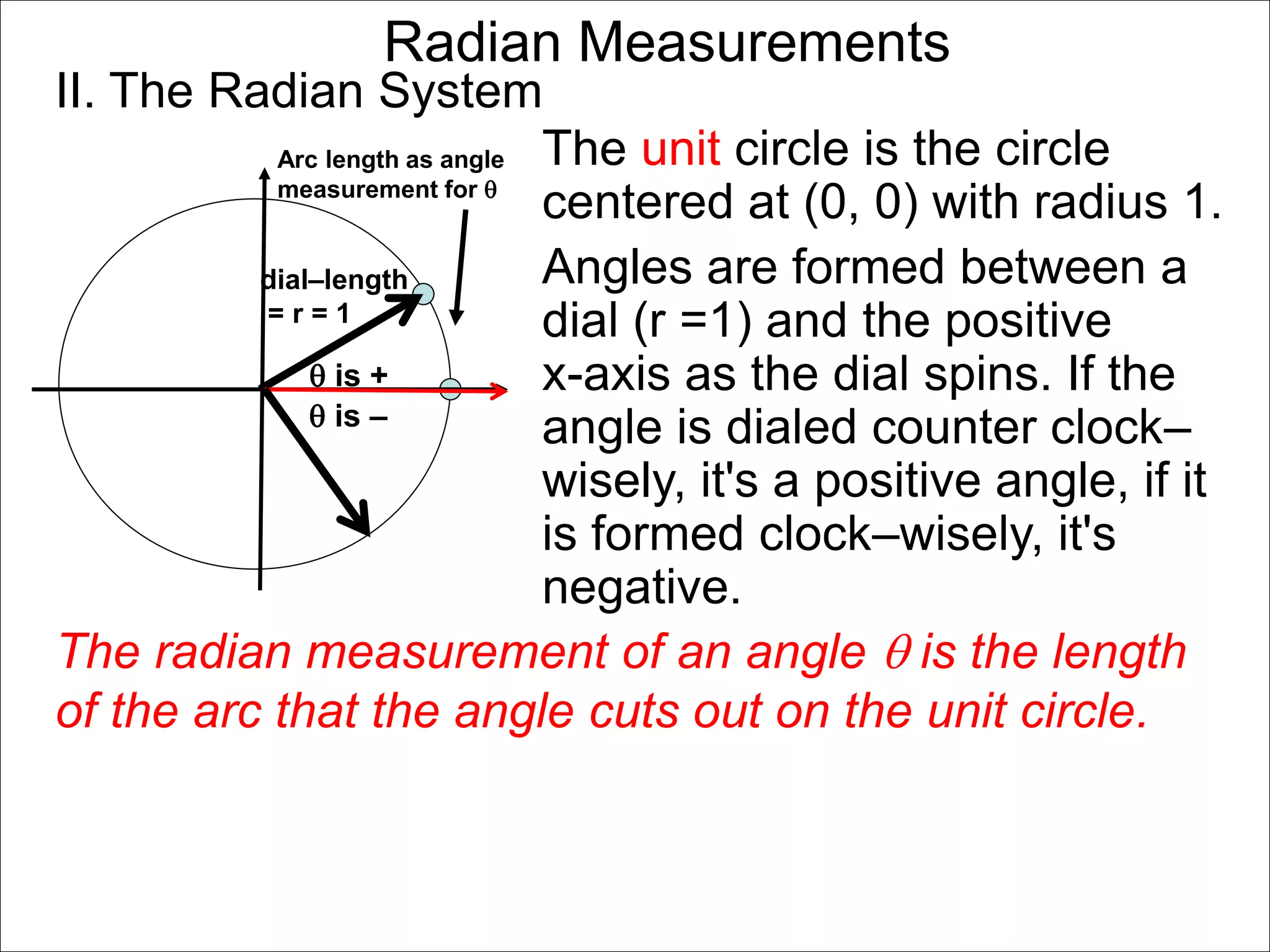
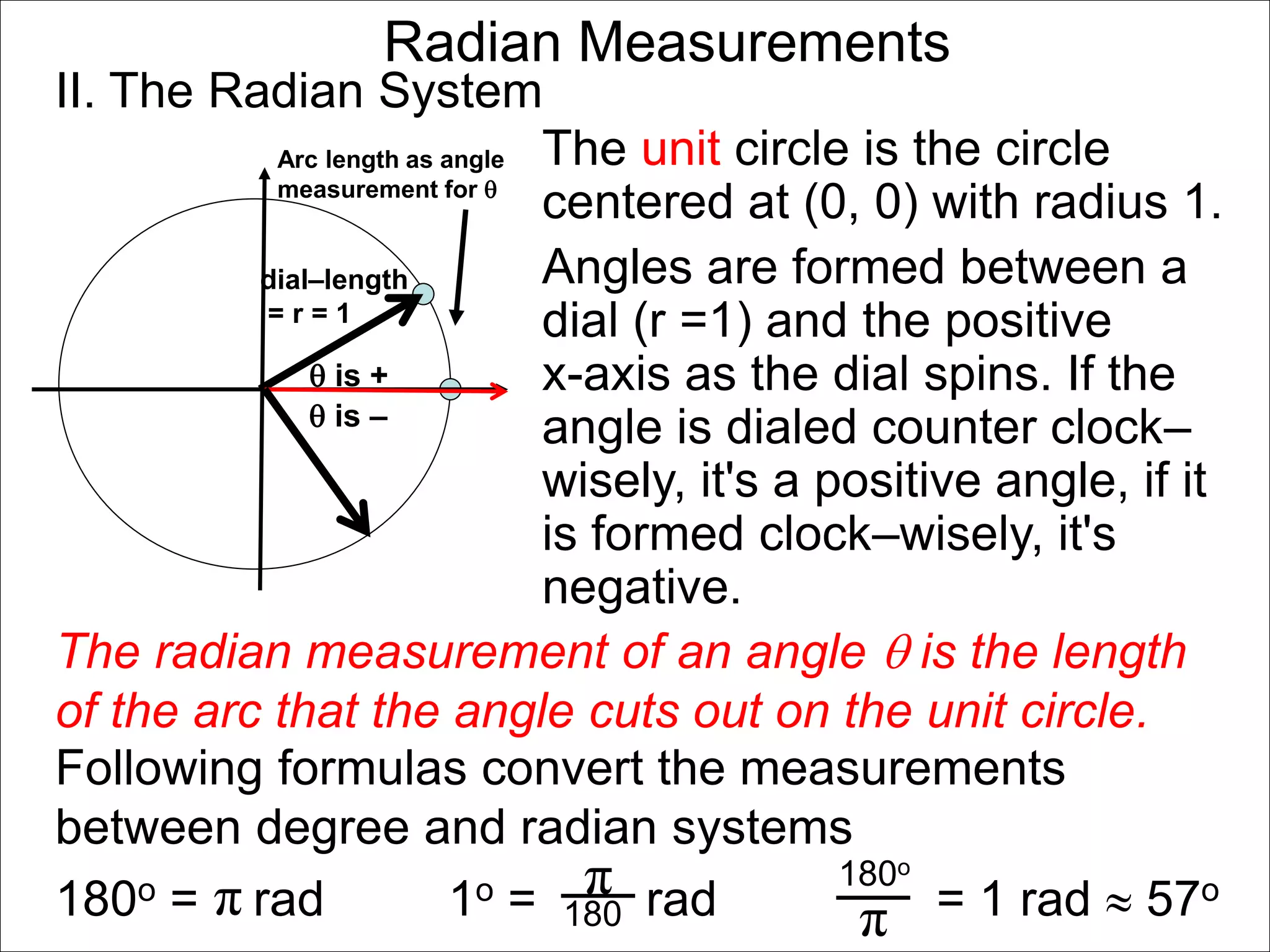
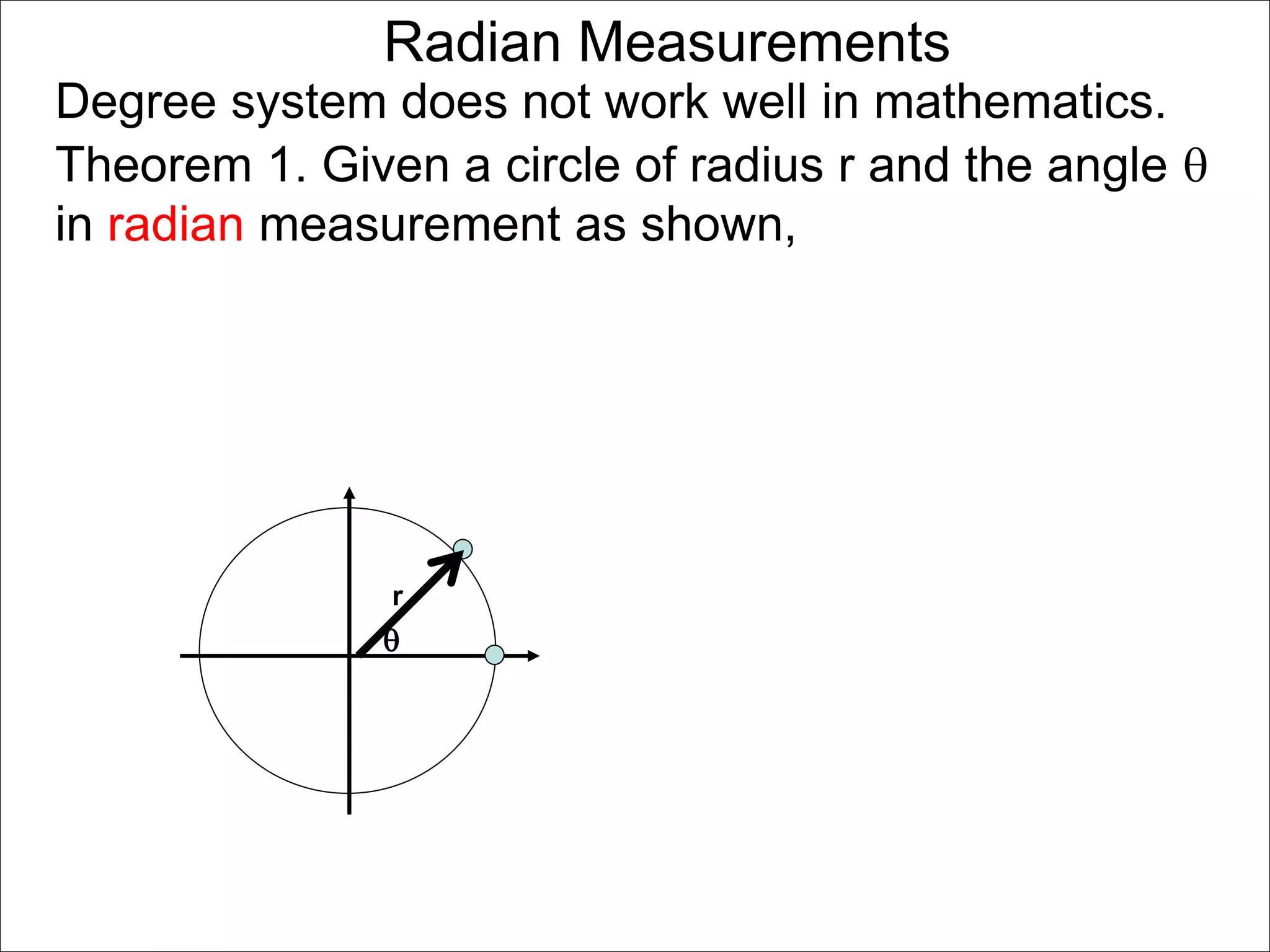
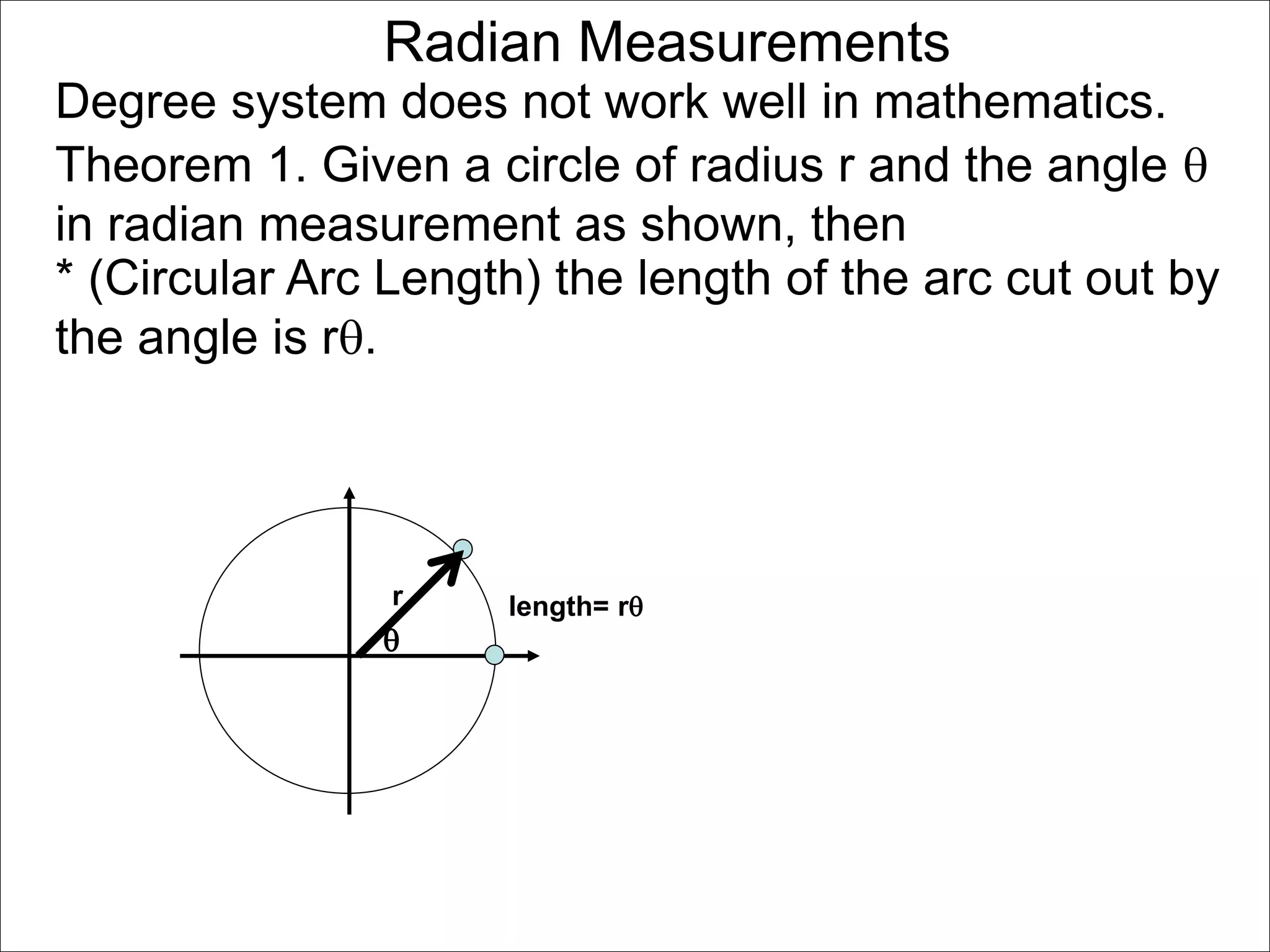
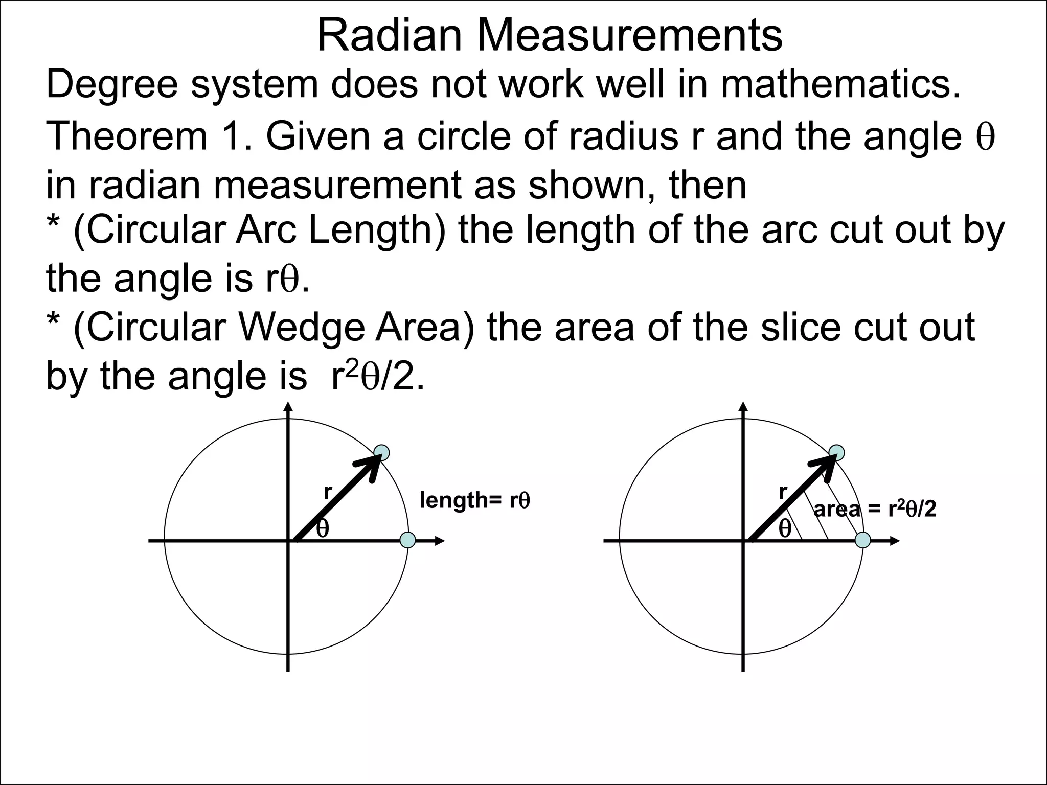
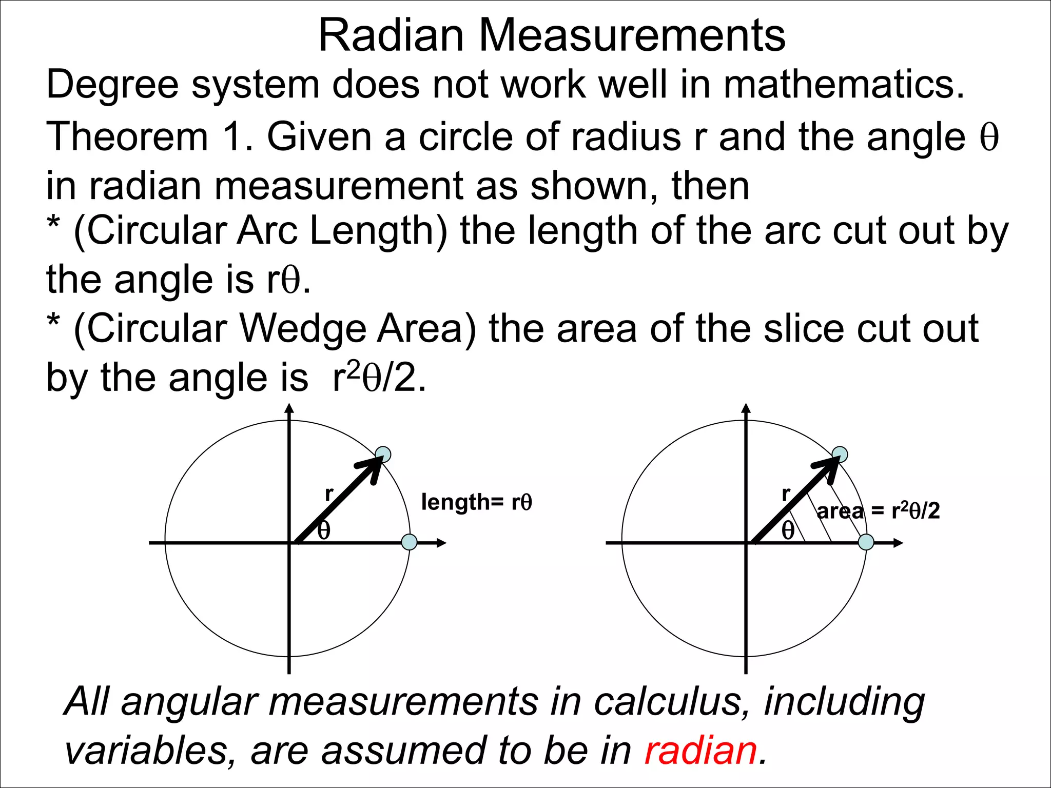
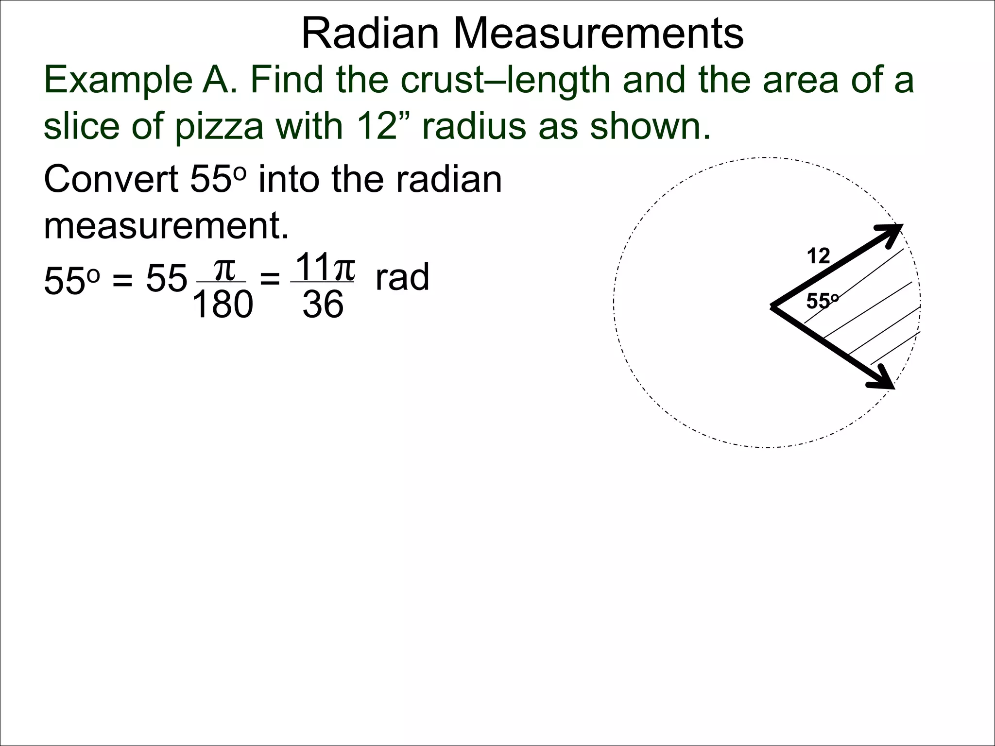
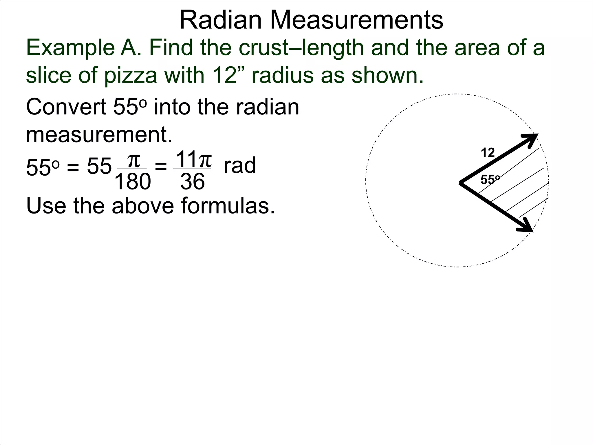
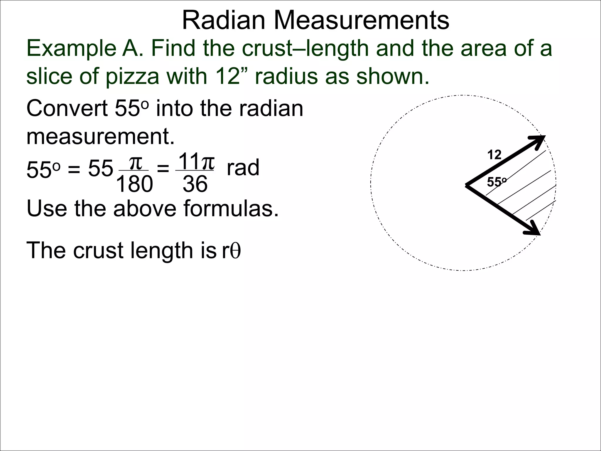
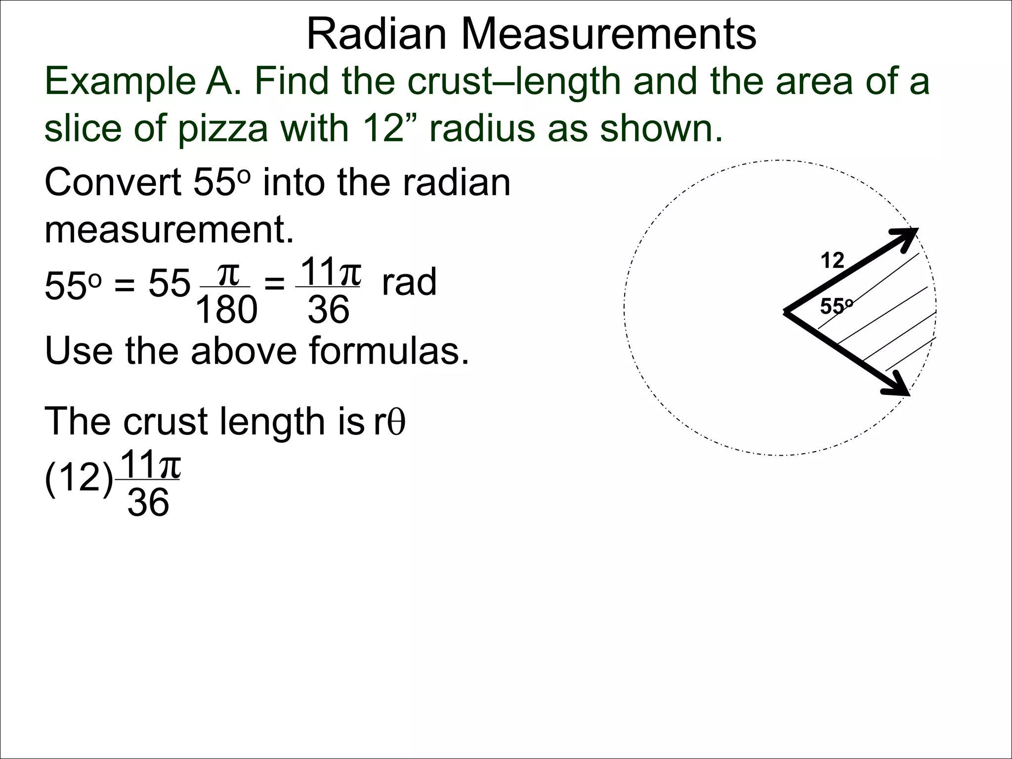
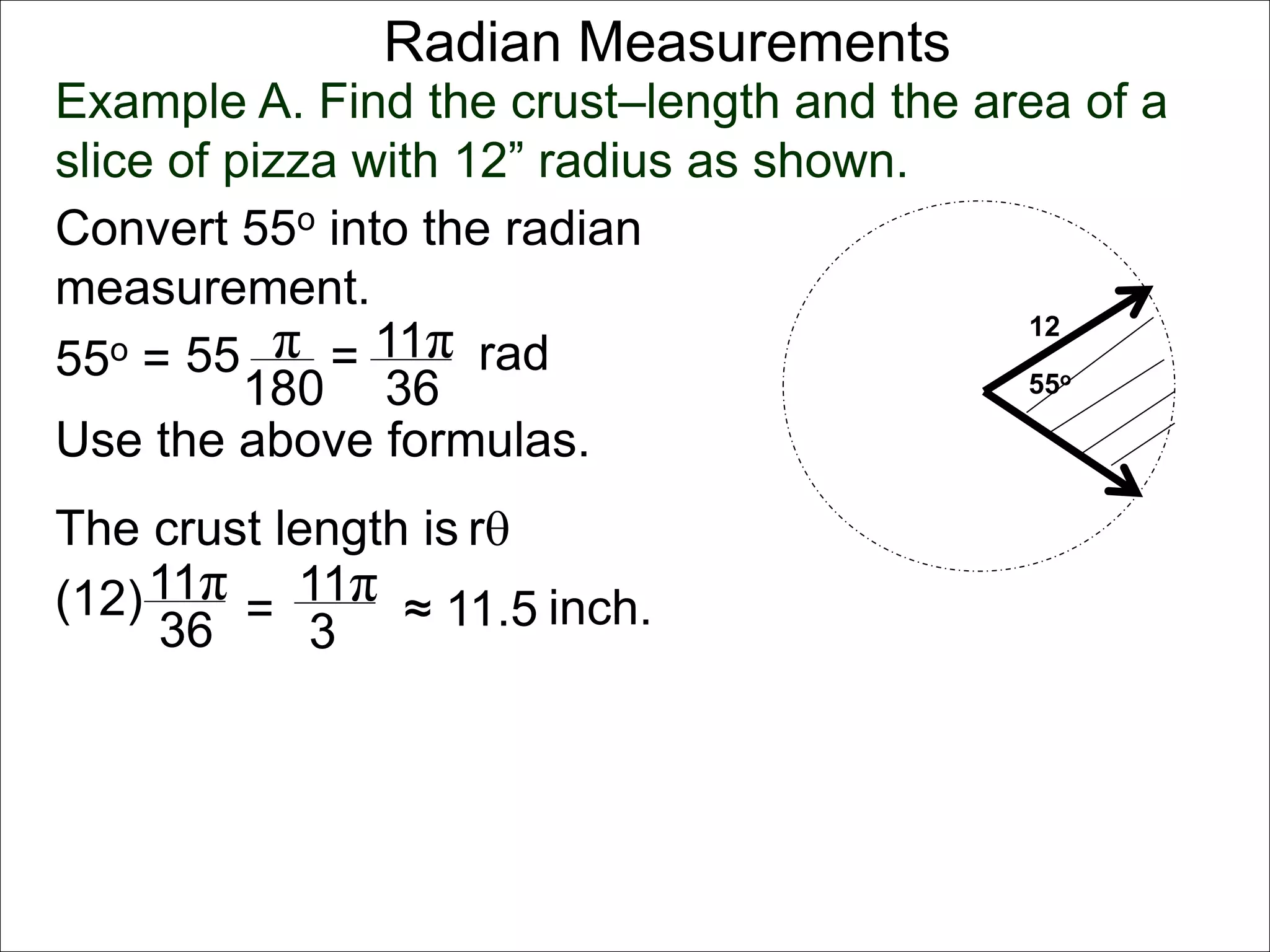
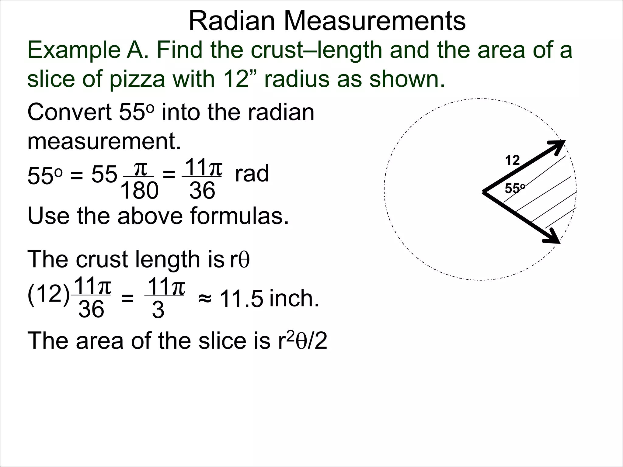
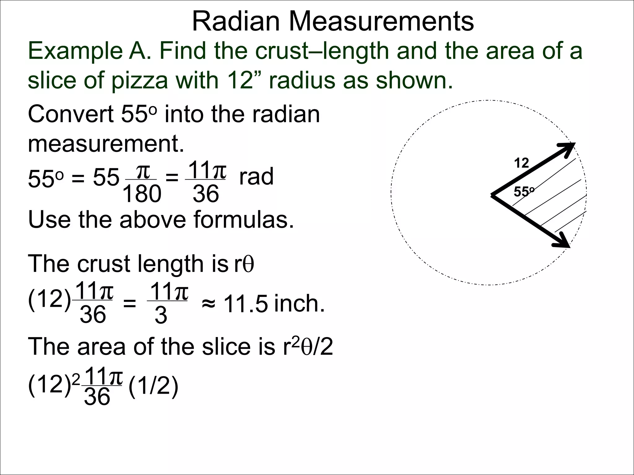
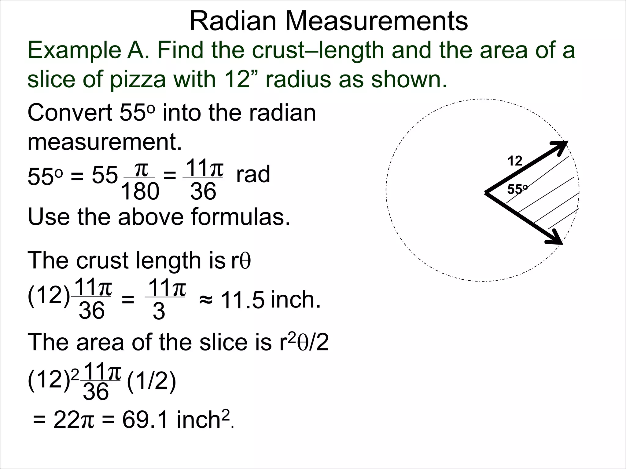
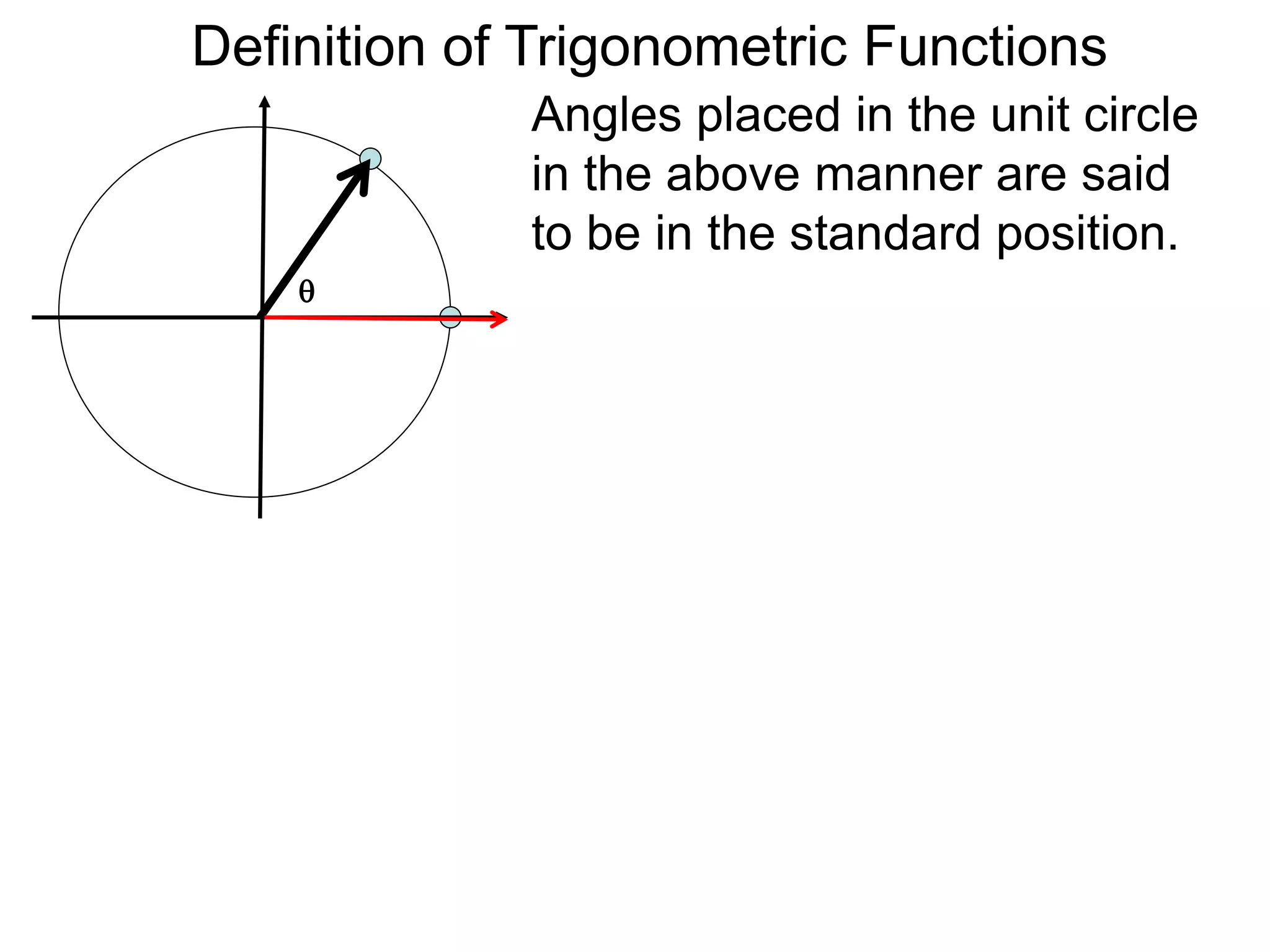
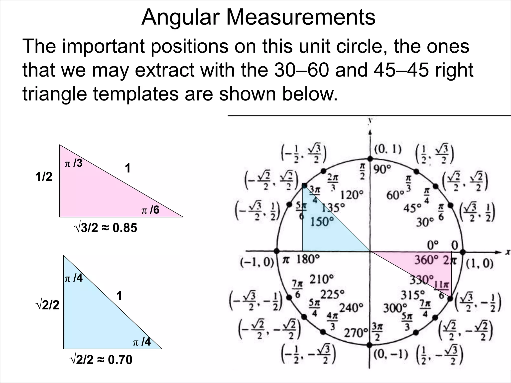
There are two systems for measuring angles: the degree system and the radian system. The degree system divides a full circle into 360 equal angles of 1 degree each. The radian system defines an angle as the arc length cut out by the angle on a unit circle of radius 1, where a full circle corresponds to 2π radians. While the degree system is commonly used, the radian system is preferred in mathematics due to its relationship to circle geometry formulas involving arc lengths and wedge areas.

1. Angular Measurements

2. Angular Measurements
There are two systems used to measure angles.

3. Angular Measurements
There are two systems used to measure angles.
I. The Degree System

4. Angular Measurements
There are two systems used to measure angles.
I. The Degree System
The degree system divides one circular angle into
360 equal angles and each is set to be 1o.

5. Angular Measurements
There are two systems used to measure angles.
I. The Degree System
The degree system divides one circular angle into
360 equal angles and each is set to be 1o.
Extend your arm fully and make a fist as though you
are handing a torch over to some one else, the
vertical visual angle of the fist is about 10o.

6. Angular Measurements
There are two systems used to measure angles.
I. The Degree System
The degree system divides one circular angle into
360 equal angles and each is set to be 1o.
Extend your arm fully and make a fist as though you
are handing a torch over to some one else, the
vertical visual angle of the fist is about 10o.
Rotate your shoulder of the out stretched
arm incrementally to the sky by stacking
the fist on top of the previous one until the
arm is pointing straight up.
It take about nine fists stacked end to end
to make the 90o rotation, so 1fist ≈ 10o.
The clinched fist measured about five
thumb–nail width. Hence 1o is
approximately the visual angle of half of
the thumb–nail width.
Your eye
10o
Your extended fist

7. Angular Measurements
There are two systems used to measure angles.
I. The Degree System
The degree system divides one circular angle into
360 equal angles and each is set to be 1o.
Extend your arm fully and make a fist as though you
are handing a torch over to some one else, the
vertical visual angle of the fist is about 10o.
One degree is divided into 60 minutes, each
minute is denoted as 1'. One minute is divided into
60 seconds, each second is denoted as 1".

8. Angular Measurements
There are two systems used to measure angles.
I. The Degree System
The degree system divides one circular angle into
360 equal angles and each is set to be 1o.
Extend your arm fully and make a fist as though you
are handing a torch over to some one else, the
vertical visual angle of the fist is about 10o.
One degree is divided into 60 minutes, each
minute is denoted as 1'. One minute is divided into
60 seconds, each second is denoted as 1".
The degree system is used mostly in science and
engineering.

9. Angular Measurements
There are two systems used to measure angles.
I. The Degree System
The degree system divides one circular angle into
360 equal angles and each is set to be 1o.
Extend your arm fully and make a fist as though you
are handing a torch over to some one else, the
vertical visual angle of the fist is about 10o.
One degree is divided into 60 minutes, each
minute is denoted as 1'. One minute is divided into
60 seconds, each second is denoted as 1".
The degree system is used mostly in science and
engineering. In mathematics, the radian system is
used because of it's relationship with the geometry
of circles.

10. Radian Measurements
II. The Radian System

11. Radian Measurements
II. The Radian System
dial–length
= r = 1
The unit circle is the circle
centered at (0, 0) with radius 1.

12. Radian Measurements
II. The Radian System
dial–length
= r = 1

The unit circle is the circle
centered at (0, 0) with radius 1.
Angles are formed between a
dial (r =1) and the positive
x-axis as the dial spins.

13. Radian Measurements
II. The Radian System
dial–length
= r = 1
 is +
The unit circle is the circle
centered at (0, 0) with radius 1.
Angles are formed between a
dial (r =1) and the positive
x-axis as the dial spins. If the
angle is dialed counter clock–
wisely, it's a positive angle,

14. Radian Measurements
II. The Radian System
dial–length
= r = 1
 is +
The unit circle is the circle
centered at (0, 0) with radius 1.
Angles are formed between a
dial (r =1) and the positive
x-axis as the dial spins. If the
angle is dialed counter clock–
wisely, it's a positive angle, if it
is formed clock–wisely, it's
negative.
 is –

15. Radian Measurements
II. The Radian System
Arc length as angle
measurement for 
dial–length
= r = 1
 is +
The unit circle is the circle
centered at (0, 0) with radius 1.
Angles are formed between a
dial (r =1) and the positive
x-axis as the dial spins. If the
angle is dialed counter clock–
wisely, it's a positive angle, if it
is formed clock–wisely, it's
negative.
 is –
The radian measurement of an angle  is the length
of the arc that the angle cuts out on the unit circle.

16. Radian Measurements
II. The Radian System
Arc length as angle
measurement for 
dial–length
= r = 1
 is +
The unit circle is the circle
centered at (0, 0) with radius 1.
Angles are formed between a
dial (r =1) and the positive
x-axis as the dial spins. If the
angle is dialed counter clock–
wisely, it's a positive angle, if it
is formed clock–wisely, it's
negative.
 is –
The radian measurement of an angle  is the length
of the arc that the angle cuts out on the unit circle.
Following formulas convert the measurements
between degree and radian systems
180o = rad 1o = rad = 1 rad  57o
π π 180o 180
π

17. Radian Measurements
Degree system does not work well in mathematics.

18. Radian Measurements
Degree system does not work well in mathematics.
Theorem 1. Given a circle of radius r and the angle 
in radian measurement as shown,
r


19. Radian Measurements
Degree system does not work well in mathematics.
Theorem 1. Given a circle of radius r and the angle 
in radian measurement as shown, then
* (Circular Arc Length) the length of the arc cut out by
the angle is r.
length= r
r


20. Radian Measurements
Degree system does not work well in mathematics.
Theorem 1. Given a circle of radius r and the angle 
in radian measurement as shown, then
* (Circular Arc Length) the length of the arc cut out by
the angle is r.
* (Circular Wedge Area) the area of the slice cut out
by the angle is r2/2.
length= r
r

area = r2/2
r


21. Radian Measurements
Degree system does not work well in mathematics.
Theorem 1. Given a circle of radius r and the angle 
in radian measurement as shown, then
* (Circular Arc Length) the length of the arc cut out by
the angle is r.
* (Circular Wedge Area) the area of the slice cut out
by the angle is r2/2.
length= r
r

area = r2/2
r

All angular measurements in calculus, including
variables, are assumed to be in radian.

22. Radian Measurements
Example A. Find the crust–length and the area of a
slice of pizza with 12” radius as shown.
12
55o

23. Radian Measurements
Example A. Find the crust–length and the area of a
slice of pizza with 12” radius as shown.
12
55o
Note that if we apply the arc length
formula using 55o directly we get a
ridiculous answer of 660” or 55’ of crust!

24. Radian Measurements
Example A. Find the crust–length and the area of a
slice of pizza with 12” radius as shown.
12
55o
Convert 55o into the radian
measurement.

25. Radian Measurements
Example A. Find the crust–length and the area of a
slice of pizza with 12” radius as shown.
12
55o
Convert 55o into the radian
measurement.
55o = 55 π
rad
180
= 11π
36

26. Radian Measurements
Example A. Find the crust–length and the area of a
slice of pizza with 12” radius as shown.
12
55o
Convert 55o into the radian
measurement.
55o = 55 π
rad
180
= 11π
36
Use the above formulas.

27. Radian Measurements
Example A. Find the crust–length and the area of a
slice of pizza with 12” radius as shown.
12
55o
Convert 55o into the radian
measurement.
55o = 55 π
rad
180
= 11π
36
Use the above formulas.
The crust length is r

28. Radian Measurements
Example A. Find the crust–length and the area of a
slice of pizza with 12” radius as shown.
12
55o
Convert 55o into the radian
measurement.
55o = 55 π
rad
180
= 11π
36
Use the above formulas.
The crust length is r
11π
36
(12)

29. Radian Measurements
Example A. Find the crust–length and the area of a
slice of pizza with 12” radius as shown.
12
55o
Convert 55o into the radian
measurement.
55o = 55 π
rad
180
= 11π
36
Use the above formulas.
The crust length is r
11π
36
(12) =
11π
3
≈ 11.5 inch.

30. Radian Measurements
Example A. Find the crust–length and the area of a
slice of pizza with 12” radius as shown.
12
55o
Convert 55o into the radian
measurement.
55o = 55 π
rad
180
= 11π
36
Use the above formulas.
The crust length is r
11π
36
(12) =
11π
3
≈ 11.5 inch.
The area of the slice is r2/2

31. Radian Measurements
Example A. Find the crust–length and the area of a
slice of pizza with 12” radius as shown.
12
55o
Convert 55o into the radian
measurement.
55o = 55 π
rad
180
= 11π
36
Use the above formulas.
The crust length is r
11π
36
(12) =
11π
3
The area of the slice is r2/2
11π
36
(12)2 (1/2)
≈ 11.5 inch.

32. Radian Measurements
Example A. Find the crust–length and the area of a
slice of pizza with 12” radius as shown.
12
55o
Convert 55o into the radian
measurement.
55o = 55 π
rad
180
= 11π
36
Use the above formulas.
The crust length is r
11π
36
(12) =
11π
3
≈ 11.5
The area of the slice is r2/2
11π
36
(12)2 (1/2)
inch.
= 22π = 69.1 inch2.

33. Definition of Trigonometric Functions
Angles placed in the unit circle
in the above manner are said
to be in the standard position.


34. Definition of Trigonometric Functions
Angles placed in the unit circle
in the above manner are said
to be in the standard position.
There are infinitely many ’s
that dial to the same position
so the tip of the dial has the
same coordinates.


35. Definition of Trigonometric Functions
Angles placed in the unit circle
in the above manner are said
to be in the standard position.
There are infinitely many ’s
that dial to the same position
so the tip of the dial has the
same coordinates.

For example, the angles π/3 and –5π/3 give the
same dial–tip position ( ½, 3 /2).

36. Definition of Trigonometric Functions
Angles placed in the unit circle
in the above manner are said
to be in the standard position.
There are infinitely many ’s
that dial to the same position
so the tip of the dial has the
same coordinates.
( ½, 3 /2)
π/3
For example, the angles π/3 and –5π/3 give the
same dial–tip position ( ½, 3 /2).

37. Definition of Trigonometric Functions
Angles placed in the unit circle
in the above manner are said
to be in the standard position.
There are infinitely many ’s
that dial to the same position
so the tip of the dial has the
same coordinates.
( ½, 3 /2)
π/3
–5π/3
For example, the angles π/3 and –5π/3 give the
same dial–tip position ( ½, 3 /2).

38. Definition of Trigonometric Functions
Angles placed in the unit circle
in the above manner are said
to be in the standard position.
There are infinitely many ’s
that dial to the same position
so the tip of the dial has the
same coordinates.
( ½, 3 /2)
π/3
–5π/3
For example, the angles π/3 and –5π/3 give the
same dial–tip position ( ½, 3 /2).
Specifically, the coordinate (x, y) of the dial–tip on
the unit circle is the same for all angles  ±2nπ
where n = 0, 1, 2, ..

39. Definition of Trigonometric Functions
Angles placed in the unit circle
in the above manner are said
to be in the standard position.
There are infinitely many ’s
that dial to the same position
so the tip of the dial has the
same coordinates.
( ½, 3 /2)
π/3
–5π/3
For example, the angles π/3 and –5π/3 give the
same dial–tip position ( ½, 3 /2).
Specifically, the coordinate (x, y) of the dial–tip on
the unit circle is the same for all angles  ±2nπ
where n = 0, 1, 2, .. Following are the definitions of
the basic trig–functions and their geometric
significances.

40. Definition of Trigonometric Functions
Given an angle  in
the standard position,
(x , y)
let (x , y) be the
coordinate of the tip
(1,0)
of the dial on the unit
 (± 2nπ)
circle.

41. Definition of Trigonometric Functions
Given an angle  in
the standard position,
let (x , y) be the
coordinate of the tip
of the dial on the unit
circle. We define
cos() = x sin() = y
tan() = cot() =
y
x
 (± 2nπ)
(x , y)
x
y
(1,0)

42. Definition of Trigonometric Functions
Given an angle  in
the standard position,
let (x , y) be the
coordinate of the tip
of the dial on the unit
circle. We define
cos() = x sin() = y
tan() = cot() =
y
x
(1,0)
(x , y)
 (± 2nπ) x=cos()
x
y

43. Definition of Trigonometric Functions
Given an angle  in
the standard position,
let (x , y) be the
coordinate of the tip
of the dial on the unit
circle. We define
cos() = x sin() = y
tan() = cot() =
y
x
(1,0)
(x , y)
 (± 2nπ) x=cos()
x
y

44. Definition of Trigonometric Functions
Given an angle  in
the standard position,
let (x , y) be the
coordinate of the tip
of the dial on the unit
circle. We define
cos() = x sin() = y
tan() = cot() =
y
x
(1,0)
(x , y)
 (± 2nπ) x=cos()
* tan() is the slope of the dial.
x
y

45. Definition of Trigonometric Functions
Given an angle  in
the standard position,
let (x , y) be the
coordinate of the tip
of the dial on the unit
circle. We define
cos() = x sin() = y
tan() = cot() =
y
x
tan()
(1,0)
(x , y)
 (± 2nπ) x=cos()
x
y
* tan() is the slope of the dial. It is called “tangent”
because tan() is the “length” of the tangent line x = 1,
from (1, 0) to the extended dial as shown.

46. Definition of Trigonometric Functions
Given an angle  in
the standard position,
let (x , y) be the
coordinate of the tip
of the dial on the unit
circle. We define
cos() = x sin() = y
tan() = cot() =
y
x
tan()
(1,0)
cot()
(x , y)
 (± 2nπ) x=cos()
x
y
* tan() is the slope of the dial. It is called “tangent”
because tan() is the “length” of the tangent line x = 1,
from (1, 0) to the extended dial as shown. Cot() is
defined similarly using the horizontal tangent y = 1.

47. Definition of Trigonometric Functions
Given an angle  in
the standard position,
let (x , y) be the
coordinate of the tip
of the dial on the unit
circle. We define
cos() = x sin() = y
tan() = cot() =
y
x
tan()
(1,0)
cot()
(x , y)
 (± 2nπ) x=cos()
x
y
* tan() is the slope of the dial. It is called “tangent”
because tan() is the “length” of the tangent line x = 1,
from (1, 0) to the extended dial as shown. Cot() is
defined similarly using the horizontal tangent y = 1.
* sin(–) = –sin() cos(–) = cos()

48. Angular Measurements
The important positions on this unit circle, the ones
that we may extract with the 30–60 and 45–45 right
triangle templates are shown below.
1
1/2
√3/2 ≈ 0.85
1
√2/2
√2/2 ≈ 0.70
π /6
π /3
π /4
π /4

49. Analytic Trigonometry
Trig–values are extracted from the unit circle so they
satisfy many algebraic relations inherited from the
equation x2 + y2 = 1 of the unit circle.

50. Analytic Trigonometry
Trig–values are extracted from the unit circle so they
satisfy many algebraic relations inherited from the
equation x2 + y2 = 1 of the unit circle. With a given
angle , replace x = cos(), y = sin(), we have the
trig–identity cos2() + sin2() = 1

51. Analytic Trigonometry
Trig–values are extracted from the unit circle so they
satisfy many algebraic relations inherited from the
equation x2 + y2 = 1 of the unit circle. With a given
angle , replace x = cos(), y = sin(), we have the
trig–identity cos2() + sin2() = 1
Just as the equation x2 + y2 = 1
may be written in multiple forms such as
1 + y2/x2 = 1/x2 or x2/y2 + 1= 1/y2

52. Analytic Trigonometry
Trig–values are extracted from the unit circle so they
satisfy many algebraic relations inherited from the
equation x2 + y2 = 1 of the unit circle. With a given
angle , replace x = cos(), y = sin(), we have the
trig–identity cos2() + sin2() = 1
Just as the equation x2 + y2 = 1
may be written in multiple forms such as
1 + y2/x2 = 1/x2 or x2/y2 + 1= 1/y2
we have correspondingly three forms of square–
sum–identities.

53. Analytic Trigonometry
Trig–values are extracted from the unit circle so they
satisfy many algebraic relations inherited from the
equation x2 + y2 = 1 of the unit circle. With a given
angle , replace x = cos(), y = sin(), we have the
trig–identity cos2() + sin2() = 1
Just as the equation x2 + y2 = 1
may be written in multiple forms such as
1 + y2/x2 = 1/x2 or x2/y2 + 1= 1/y2
we have correspondingly three forms of square–
sum–identities.
These square–sum formulas, the reciprocal and
divisional relations, are summarized by the Trig–
Wheel given below and these identities are called
the basic–trig–identities.

54. Analytic Trigonometry
The Trig-Wheel

55. Analytic Trigonometry
The Trig-Wheel
the regular-side the co-side

56. Analytic Trigonometry
The Division and
Reciprocal Relations
Start from any function,
go around the rim, then
I = II / III or I * III = II
The Trig-Wheel

57. Analytic Trigonometry
The Division and
Reciprocal Relations
Start from any function,
go around the rim, then
I = II / III or I * III = II
The Trig-Wheel
I
II III

58. Analytic Trigonometry
The Division and
Reciprocal Relations
Start from any function,
go around the rim, then
I = II / III or I * III = II
The Trig-Wheel
I
II III
Following are some important divisional relations.
tan(A) = sin(A)/cos(A)

59. Analytic Trigonometry
The Division and
Reciprocal Relations
Start from any function,
go around the rim, then
I = II / III or I * III = II
The Trig-Wheel
I
II III
Following are some important divisional relations.
tan(A) = sin(A)/cos(A) cot(A) = cos(A)/sin(A)

60. Analytic Trigonometry
The Division and
Reciprocal Relations
Start from any function,
go around the rim, then
I = II / III or I * III = II
The Trig-Wheel
I
II III
or go straight through the
center then I = 1 / III, i.e.
two formulas on opposite
ends are reciprocals.
Following are some important divisional relations.
tan(A) = sin(A)/cos(A) cot(A) = cos(A)/sin(A)

61. Analytic Trigonometry
The Division and
Reciprocal Relations
Start from any function,
go around the rim, then
I = II / III or I * III = II
The Trig-Wheel
I
II III
or go straight through the
center then I = 1 / III, i.e.
two formulas on opposite
ends are reciprocals.
Following are some important divisional relations.
tan(A) = sin(A)/cos(A) cot(A) = cos(A)/sin(A)
csc(A) = 1/sin(A) sec(A) = 1/cos(A)
cot(A) = 1/tan(A)

62. Analytic Trigonometry
The Trig-Wheel Square-Sum Relations
For each of the three inverted
triangles in the wheel, the
sum of the squares of the top
two functions is the square of
the bottom function.

63. Analytic Trigonometry
The Trig-Wheel Square-Sum Relations
For each of the three inverted
triangles in the wheel, the
sum of the squares of the top
two functions is the square of
the bottom function.
sin2(A) + cos2(A)=1
tan2(A) + 1 = sec2(A)
1 + cot2(A) = csc2(A)

64. Analytic Trigonometry
The Trig-Wheel Square-Sum Relations
For each of the three inverted
triangles in the wheel, the
sum of the squares of the top
two functions is the square of
the bottom function.
sin2(A) + cos2(A)=1
tan2(A) + 1 = sec2(A)
1 + cot2(A) = csc2(A)
Sum & Difference of Angle Formulas
Let A and B be angles then
C(A±B) = C(A)C(B) + – S(A)S(B)
S(A±B) = S(A)C(B) ± S(B)C(A)
where S(x) = sin(x) and C(x) = cos(x).

65. Analytic Trigonometry
The following are consequences of the sum and
difference formulas.
Double-Angle Formulas
S(2A) = 2S(A)C(A)
C(2A) = C2(A) – S2(A)
= 2C2(A) – 1
= 1 – 2S2(A)
Half-Angle Formulas
1 + C(B)
2
B
2
C( ) =
±
1 – C(B)
2
B
2
S( ) = ±
From the C(2A) formulas we have the following.
S2(A) =
1 – C(2A)
2
C2(A) = 1 + C(2A)
2
HW. Derive all the formulas on this page from the
Sum and Difference Formula.