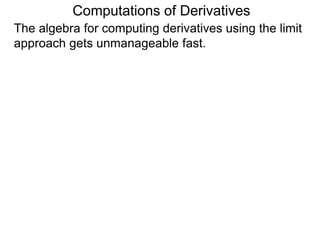
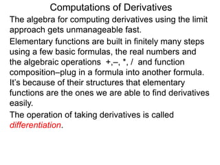
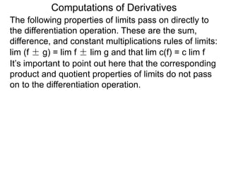
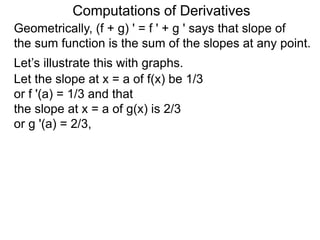
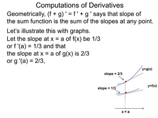
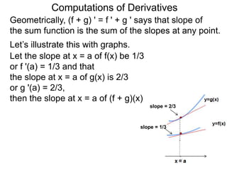
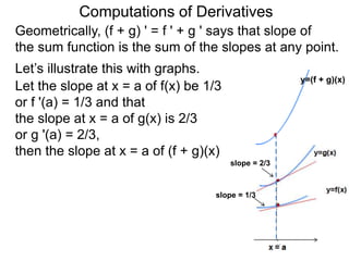
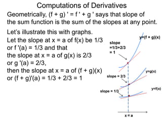
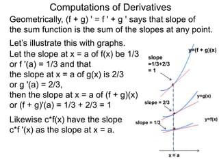
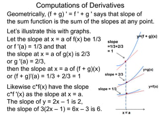
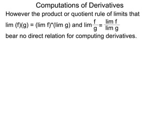
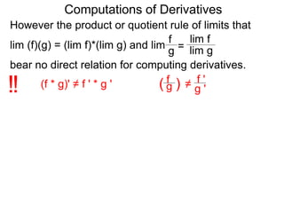
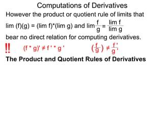
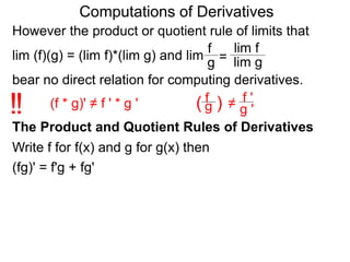
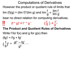
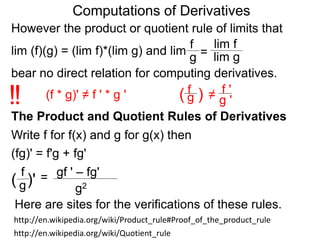
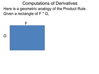
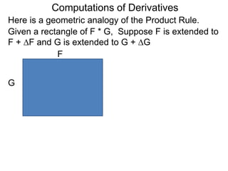
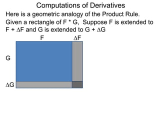
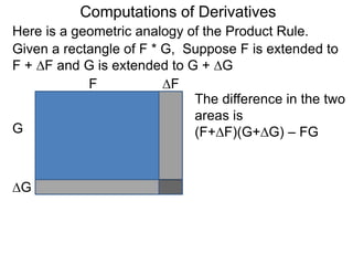
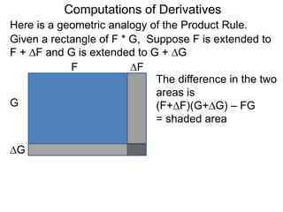
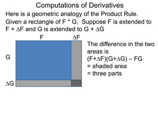
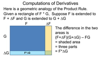
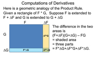
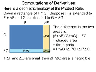
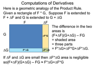
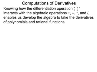
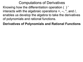
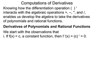
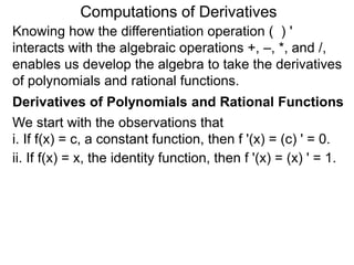
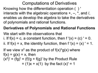
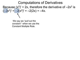
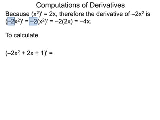
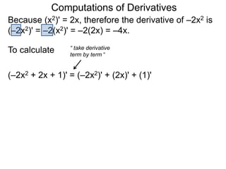
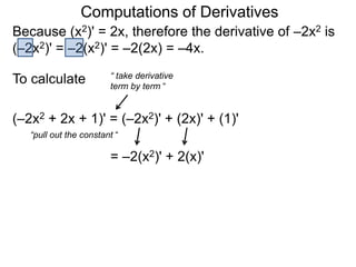
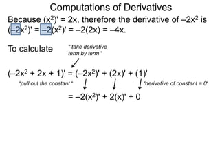
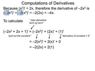
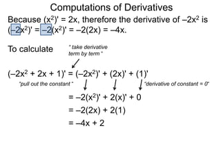
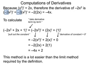
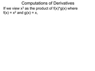
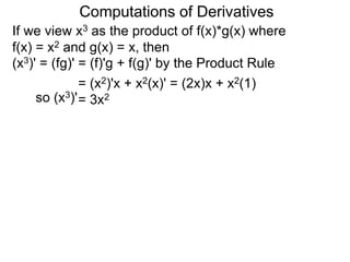
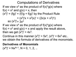
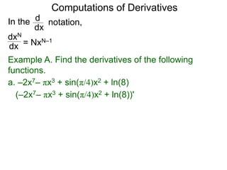
The document discusses properties of derivatives and how they relate to limits. It states that the sum, difference, and constant multiple rules for limits directly apply to differentiation. However, the product and quotient rules for limits do not directly apply to differentiation, which has more complicated product and quotient rules. Elementary functions are defined in terms of a few basic formulas and operations. The document then examines the sum and constant multiple rules for derivatives in more detail, proving them using limits. It also provides a geometric illustration of how the derivative of a sum is equal to the sum of the derivatives.
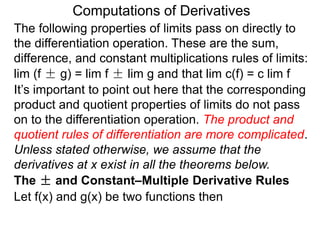
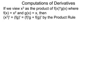
![Computations of Derivatives
To verify i, note that
lim
[f(x+h) + g(x+h)] – [f(x) + g(x)]
h →0 h
=
(f(x) + g(x)) '](https://image.slidesharecdn.com/2-5computationsofderivatives-120303132727-phpapp01/85/2-5-computations-of-derivatives-17-320.jpg)
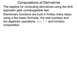
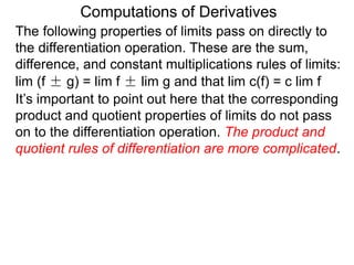
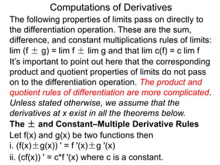
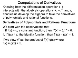
![Computations of Derivatives
To verify i, note that
lim
[f(x+h) + g(x+h)] – [f(x) + g(x)]
h →0 h
=
(f(x) + g(x)) '
lim [f(x+h) – f(x)] + [g(x+h) – g(x)]
h h →0
=](https://image.slidesharecdn.com/2-5computationsofderivatives-120303132727-phpapp01/85/2-5-computations-of-derivatives-18-320.jpg)
![Computations of Derivatives
To verify i, note that
lim
[f(x+h) + g(x+h)] – [f(x) + g(x)]
h →0 h
=
(f(x) + g(x)) '
lim [f(x+h) – f(x)] + [g(x+h) – g(x)]
h h →0
=
lim [f(x+h) – f(x)] [g(x+h) – g(x)]
= +
h
h →0
h](https://image.slidesharecdn.com/2-5computationsofderivatives-120303132727-phpapp01/85/2-5-computations-of-derivatives-19-320.jpg)
![Computations of Derivatives
To verify i, note that
lim
[f(x+h) + g(x+h)] – [f(x) + g(x)]
h →0 h
=
(f(x) + g(x)) '
lim [f(x+h) – f(x)] + [g(x+h) – g(x)]
h h →0
=
lim [f(x+h) – f(x)] [g(x+h) – g(x)]
= +
h
h →0
h
(the sum property of limits)
lim [f(x+h) – f(x)]
h h →0 = +
lim [g(x+h) – g(x)]
h →0
h](https://image.slidesharecdn.com/2-5computationsofderivatives-120303132727-phpapp01/85/2-5-computations-of-derivatives-20-320.jpg)
![Computations of Derivatives
To verify i, note that
lim
[f(x+h) + g(x+h)] – [f(x) + g(x)]
h →0 h
=
(f(x) + g(x)) '
lim [f(x+h) – f(x)] + [g(x+h) – g(x)]
h h →0
=
lim [f(x+h) – f(x)] [g(x+h) – g(x)]
= +
h
h →0
h
(the sum property of limits)
lim [f(x+h) – f(x)]
h h →0 = +
lim [g(x+h) – g(x)]
h →0
h
= f '(x) + g '(x)](https://image.slidesharecdn.com/2-5computationsofderivatives-120303132727-phpapp01/85/2-5-computations-of-derivatives-21-320.jpg)
![Computations of Derivatives
To verify i, note that
lim
[f(x+h) + g(x+h)] – [f(x) + g(x)]
h →0 h
=
(f(x) + g(x)) '
lim [f(x+h) – f(x)] + [g(x+h) – g(x)]
h h →0
=
lim [f(x+h) – f(x)] [g(x+h) – g(x)]
= +
h
h →0
h
(the sum property of limits)
lim [f(x+h) – f(x)]
h h →0 = +
lim [g(x+h) – g(x)]
h →0
h
= f '(x) + g '(x)
Your turn: Verity part ii in a similar manner.](https://image.slidesharecdn.com/2-5computationsofderivatives-120303132727-phpapp01/85/2-5-computations-of-derivatives-22-320.jpg)


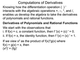
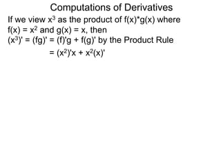
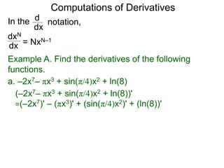
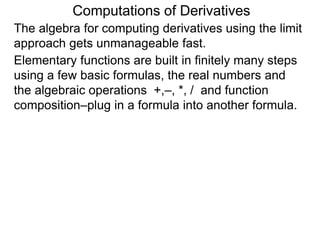
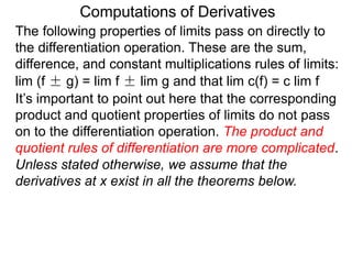
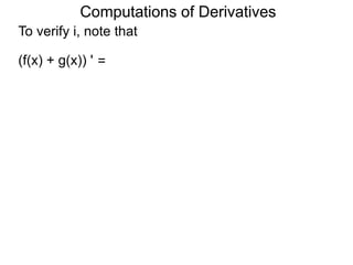
![Computations of Derivatives
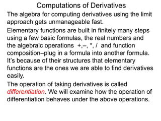
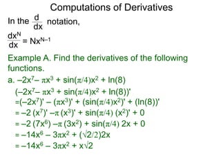
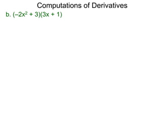
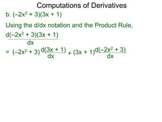
b. (–2x2 + 3)(3x + 1)
Using the d/dx notation and the Product Rule,
d(–2x2 + 3)(3x + 1)
dx
= (–2x2 + 3) d(3x + 1)
dx +
d(–2x2 + 3)
dx
(3x + 1)
= (–2x2 + 3)(3 + 0) + (3x + 1)(–4x + 0)
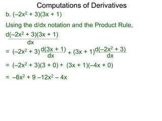
= –6x2 + 9 –12x2 – 4x
= –18x2 – 4x + 9
or that [(–2x2 + 3)(3x + 1)] '
= (–6x3 – 2x2 + 9x + 3)'](https://image.slidesharecdn.com/2-5computationsofderivatives-120303132727-phpapp01/85/2-5-computations-of-derivatives-94-320.jpg)
![Computations of Derivatives
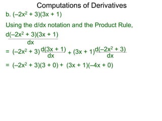
b. (–2x2 + 3)(3x + 1)
Using the d/dx notation and the Product Rule,
d(–2x2 + 3)(3x + 1)
dx
= (–2x2 + 3) d(3x + 1)
dx +
d(–2x2 + 3)
dx
(3x + 1)
= (–2x2 + 3)(3 + 0) + (3x + 1)(–4x + 0)
= –6x2 + 9 –12x2 – 4x
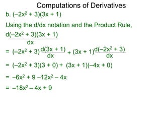
= –18x2 – 4x + 9
or that [(–2x2 + 3)(3x + 1)] '
= (–6x3 – 2x2 + 9x + 3)' = –18x2 – 4x + 9](https://image.slidesharecdn.com/2-5computationsofderivatives-120303132727-phpapp01/85/2-5-computations-of-derivatives-95-320.jpg)
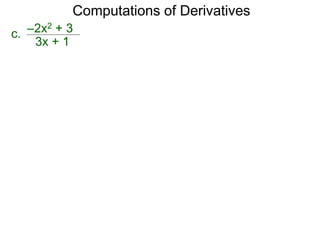
![Computations of Derivatives
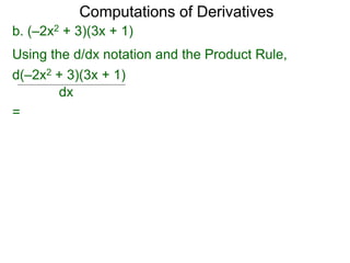
c. –2x2 + 3
Use the Quotient Rule
=
3x + 1
–2x2 + 3
3x + 1 [ ]'
gf ' – fg'
g2
f
( g )'=](https://image.slidesharecdn.com/2-5computationsofderivatives-120303132727-phpapp01/85/2-5-computations-of-derivatives-97-320.jpg)
![Computations of Derivatives
c. –2x2 + 3
=
3x + 1
–2x2 + 3
3x + 1 [ ]'
(3x + 1)2
Use the Quotient Rule
gf ' – fg'
g2
f
( g )'=](https://image.slidesharecdn.com/2-5computationsofderivatives-120303132727-phpapp01/85/2-5-computations-of-derivatives-98-320.jpg)
![Computations of Derivatives
c. –2x2 + 3
=
3x + 1
–2x2 + 3
3x + 1 [ ]'
(3x + 1)(–2x2 + 3)'
(3x + 1)2
Use the Quotient Rule
gf ' – fg'
g2
f
( g )'=](https://image.slidesharecdn.com/2-5computationsofderivatives-120303132727-phpapp01/85/2-5-computations-of-derivatives-99-320.jpg)
![Computations of Derivatives
c. –2x2 + 3
=
3x + 1
–2x2 + 3
3x + 1 [ ]'
(3x + 1)(–2x2 + 3)' – (–2x2 + 3)(3x + 1)'
(3x + 1)2
Use the Quotient Rule
gf ' – fg'
g2
f
( g )'=](https://image.slidesharecdn.com/2-5computationsofderivatives-120303132727-phpapp01/85/2-5-computations-of-derivatives-100-320.jpg)
![Computations of Derivatives
c. –2x2 + 3
=
3x + 1
–2x2 + 3
3x + 1 [ ]'
(3x + 1)(–2x2 + 3)' – (–2x2 + 3)(3x + 1)'
(3x + 1)2
Use the Quotient Rule
gf ' – fg'
g2
f
( g )'=
(3x + 1)(–4x) – (–2x2 + 3)(3)
(3x + 1)2
=](https://image.slidesharecdn.com/2-5computationsofderivatives-120303132727-phpapp01/85/2-5-computations-of-derivatives-101-320.jpg)
![Computations of Derivatives
c. –2x2 + 3
=
3x + 1
–2x2 + 3
3x + 1 [ ]'
(3x + 1)(–2x2 + 3)' – (–2x2 + 3)(3x + 1)'
(3x + 1)2
Use the Quotient Rule
gf ' – fg'
g2
f
( g )'=
(3x + 1)(–4x) – (–2x2 + 3)(3)
(3x + 1)2
=
–12x2 – 4x + 6x2 – 9
(3x + 1)2
=](https://image.slidesharecdn.com/2-5computationsofderivatives-120303132727-phpapp01/85/2-5-computations-of-derivatives-102-320.jpg)
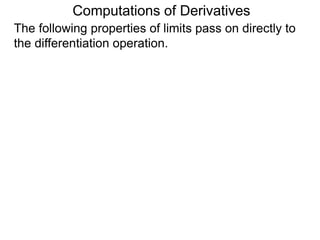
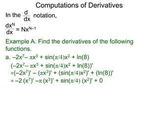
![Computations of Derivatives
c. –2x2 + 3
=
3x + 1
–2x2 + 3
3x + 1 [ ]'
(3x + 1)(–2x2 + 3)' – (–2x2 + 3)(3x + 1)'
(3x + 1)2
Use the Quotient Rule
gf ' – fg'
g2
f
( g )'=
(3x + 1)(–4x) – (–2x2 + 3)(3)
(3x + 1)2
=
–12x2 – 4x + 6x2 – 9
(3x + 1)2
=
–6x2 – 4x – 9
(3x + 1)2
=](https://image.slidesharecdn.com/2-5computationsofderivatives-120303132727-phpapp01/85/2-5-computations-of-derivatives-103-320.jpg)
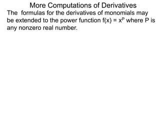
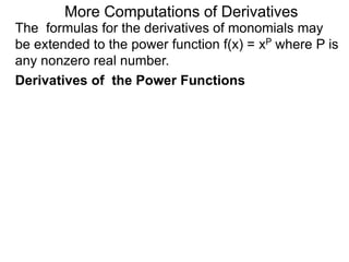
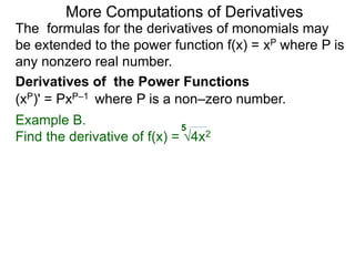
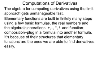
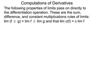
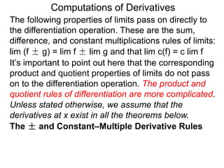
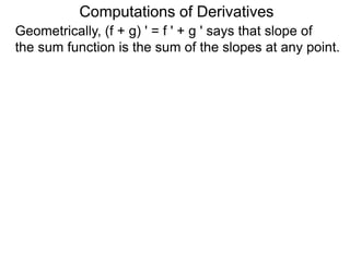
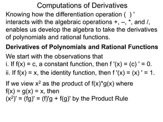
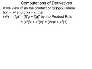
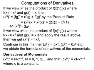
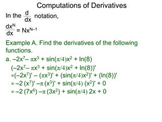
![More Computations of Derivatives
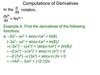
The formulas for the derivatives of monomials may
be extended to the power function f(x) = xP where P is
any nonzero real number.
Derivatives of the Power Functions
(xP)' = PxP–1 where P is a non–zero number.
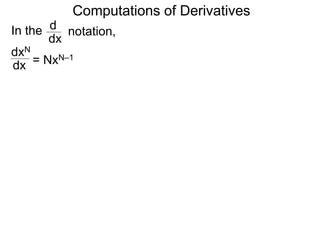
Example B.
5
Find the derivative of f(x) = √4x2
5
(√4x2)'
= [(4x2)1/5] '](https://image.slidesharecdn.com/2-5computationsofderivatives-120303132727-phpapp01/85/2-5-computations-of-derivatives-108-320.jpg)
![More Computations of Derivatives
The formulas for the derivatives of monomials may
be extended to the power function f(x) = xP where P is
any nonzero real number.
Derivatives of the Power Functions
(xP)' = PxP–1 where P is a non–zero number.
Example B.
5
Find the derivative of f(x) = √4x2
5
(√4x2)'
= [(4x2)1/5] '
= [41/5x2/5] '](https://image.slidesharecdn.com/2-5computationsofderivatives-120303132727-phpapp01/85/2-5-computations-of-derivatives-109-320.jpg)
![More Computations of Derivatives
The formulas for the derivatives of monomials may
be extended to the power function f(x) = xP where P is
any nonzero real number.
Derivatives of the Power Functions
(xP)' = PxP–1 where P is a non–zero number.
Example B.
5
Find the derivative of f(x) = √4x2
5
(√4x2)'
= [(4x2)1/5] '
= [41/5x2/5] '
= 41/5 [x2/5] '](https://image.slidesharecdn.com/2-5computationsofderivatives-120303132727-phpapp01/85/2-5-computations-of-derivatives-110-320.jpg)
![More Computations of Derivatives
The formulas for the derivatives of monomials may
be extended to the power function f(x) = xP where P is
any nonzero real number.
Derivatives of the Power Functions
(xP)' = PxP–1 where P is a non–zero number.
Example B.
5
Find the derivative of f(x) = √4x2
5
(√4x2)'
= [(4x2)1/5] '
= [41/5x2/5] '
= 41/5 [x2/5] '
= 41/5 [ 2 x2/5 – 1]
5](https://image.slidesharecdn.com/2-5computationsofderivatives-120303132727-phpapp01/85/2-5-computations-of-derivatives-111-320.jpg)
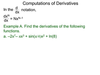
![More Computations of Derivatives
The formulas for the derivatives of monomials may
be extended to the power function f(x) = xP where P is
any nonzero real number.
Derivatives of the Power Functions
(xP)' = PxP–1 where P is a non–zero number.
Example B.
5
Find the derivative of f(x) = √4x2
5
(√4x2)'
= [(4x2)1/5] '
= [41/5x2/5] '
= 41/5 [x2/5] '
= 41/5 [ 2 x2/5 – 1]
5
(41/5)
= 2 x –3/5
5](https://image.slidesharecdn.com/2-5computationsofderivatives-120303132727-phpapp01/85/2-5-computations-of-derivatives-112-320.jpg)