* tuning gradient boosting over decision trees (GBDT) * speeding up predictions for online triggers: lookup tables * PCA, autoencoder, manifold learning * structural learning: Markov chain, LDA * remarks on collaborative research

1. MACHINE LEARNING IN HIGH
ENERGY PHYSICS
LECTURE #4
Alex Rogozhnikov, 2015

2. WEIGHTED VOTING
The way to introduce importance of classifiers
D(x) = (x)∑j
αj dj
GENERAL CASE OF ENSEMBLING:
D(x) = f ( (x), (x), …, (x))d1 d2 dJ

3. COMPARISON OF DISTRIBUTIONS
good options to compare 1d
use classifier's output to build discriminating variable
ROC AUC + Mann Whitney to get significance

5. RANDOM FOREST
composition of independent trees

6. ADABOOST
After building th base classifier:j
1.
2. increase weight of misclassified
= ln
( )
αj
1
2
wcorrect
wwrong
← ×wi wi e
− ( )αj yi
dj xi

8. GRADIENT BOOSTING
 → min
(x) = (x)Dj ∑j
=1j
′ αj
′ dj
′
(x) = (x) + (x)Dj Dj−1 αj dj
At th iteration:j
pseudo-residual
train regressor to minimize MSE:
find optimal
= − zi
∂
∂D( )xi
∣∣D(x)= (x)Dj−1
dj
( ( ) − → min∑i
dj xi zi )
2
αj

9. LOSSES
regression,
Mean Squared Error
Mean Absolute Error
binary classification,
ExpLoss (aka AdaLoss)
LogLoss
ranking losses
boosting to uniformity: FlatnessLoss
y ∈ ℝ
(d( ) −∑i
xi yi )
2
d( ) −∑i
∣∣ xi yi
∣∣
= ±1yi
∑i
e
− d( )yi
xi
log(1 + )∑i
e
− d( )yi
xi

10. TUNING GRADIENT BOOSTING OVER
DECISION TREES
Parameters:
loss function
pre-pruning: maximal depth, minimal leaf size
subsample, max_features =
(learning_rate)
number of trees
N/3
η

11. LOSS FUNCTION
different combinations also may be used

14. TUNING GBDT
1. set high, but feasible number of trees
2. find optimal parameters by checking combinations
3. decrease learning rate, increase number of trees
See also: GBDT tutorial

15. BaggingClassifier(base_estimator=GradientBoostingClassifier(),
n_estimators=100)
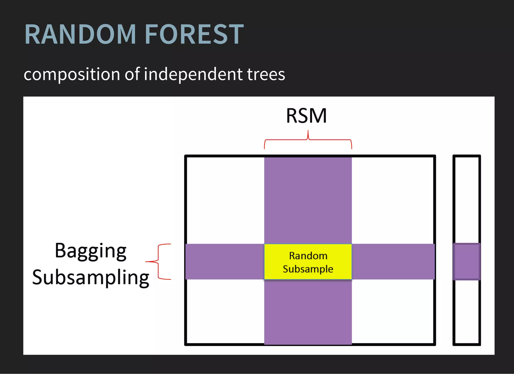
ENSEMBLES: BAGGING OVER
BOOSTING
Different variations , are claimed to overcome single
GBDT.
[1] [2]
Very complex training, better quality if GB estimators are
overfitted

16. ENSEMBLES: STACKING
Correcting output of several classifiers with new classifier.
D(x) = f ( (x), (x), …, (x))d1 d2 dJ
To use unbiased predictions, use holdout or kFolding.

17. REWEIGHTING
Given two distributions: target and original, find new
weights for original distributions, that distributions will
coincide.

19. REWEIGHTING
Solution for 1 or 2 variables: reweight using bins (so-called
'histogram division').
Typical application: Monte-Carlo reweighting.

20. REWEIGHTING WITH BINS
Splitting all space in bins, for each bin:
compute , in each bin
multiply weights of original distribution in bin to
compensate the difference
woriginal wtarget
←wi wi
wtarget
woriginal
Problems
good in 1d, works sometimes in 2d, nearly impossible in
dimensions > 2
too few events in bin reweighting rule is unstable
we can reweight several times over 1d if variables aren't
correlated
⇒

21. reweighting using enhanced version of bin reweighter

22. reweighting using gradient boosted reweighter

23. GRADIENT BOOSTED REWEIGHTER
works well in high dimensions
works with correlated variables
produces more stable reweighting rule

24. HOW DOES GB REWEIGHTER
WORKS?
iteratively:
1. Find the tree, which is able to discriminate two distributions
2. Correct weights in each leaf
3. Reweight original distribution and repeat the process.
Less bins, bins are guaranteed to have high statistic in each.

25. DISCRIMINATING TREE
When looking for a tree with good discrimination, optimize
=χ2
∑l∈leaves
( −wl,target wl,original )
2
+wl,target wl,original
As before, using greedy minimization to build a tree, which
provides maximal .χ2
+ introducing all heuristics from standard GB.

26. QUALITY ESTIMATION
Quality of model can be estimated by the value of optimized
loss function. Though remember that different classifiers
use different optimization target
LogLoss ExpLoss

27. QUALITY ESTIMATION
different target of optimization use general quality
metrics
⇒

28. TESTING HYPOTHESIS WITH CUT
Example: we test hypothesis that there is signal channel
with fixed vs. no signal channel ( ).Br ≠ 0 Br = 0
: signal channel with
: there is no signal channel
H0 Br = const
H1
Putting a threshold: d(x) > threshold
Estimate number of signal / bkg events that will be selected:
s = α tpr, b = β fpr
:
:
H0 ∼ Poiss(s + b)nobs
H1 ∼ Poiss(b)nobs

29. TESTING HYPOTHESIS WITH CUT
Select some appropriate metric:
= 2(s + b) log(1 + ) − 2sAMS
2
s
b
Maximize it by selecting best
special holdout shall be used
or use kFolding
very poor usage of information from classifier
threshold

30. TESTING HYPOTHESIS WITH BINS
Splitting all data in bins:
.
n
x ∈ k-th bin ⇔ < d(x) ≤thrk−1 thrk
Expected amounts of signal:
= α( − ), = β( − )sk tpr
k−1
tpr
k
bk fpr
k−1
fpr
k
:
:
H0 ∼ Poiss( + )nk sk bk
H1 ∼ Poiss( )nk bk
Optimal statistics:
, = log(1 + )
∑
k
ck nk ck
sk
bk
take some approximation to test power and optimize
thresholds

31. FINDING OPTIMAL PARAMETERS
some algorithms have many parameters
not all the parameters are guessed
checking all combinations takes too long

32. FINDING OPTIMAL PARAMETERS
randomly picking parameters is a partial solution
given a target optimal value we can optimize it
no gradient with respect to parameters
noisy results
function reconstruction is a problem
Before running grid optimization make sure your metric is
stable (i.e. by train/testing on different subsets).
Overfitting by using many attempts is real issue.

33. OPTIMAL GRID SEARCH
stochastic optimization (Metropolis-Hastings, annealing)
regression techniques, reusing all known information
(ML to optimize ML!)

34. OPTIMAL GRID SEARCH USING
REGRESSION
General algorithm (point of grid = set of parameters):
1. evaluations at random points
2. build regression model based on known results
3. select the point with best expected quality according to
trained model
4. evaluate quality at this points
5. Go to 2 if not enough evaluations
Why not using linear regression?

35. GAUSSIAN PROCESSES FOR
REGRESSION
Some definitions: , where and are
functions of mean and covariance: ,
Y ∼ GP(m, K) m K
m(x) K( , )x1 x2
represents our prior expectation of quality
(may taken constant)
represents influence of known
results on expectation of new
RBF kernel is the most useful:
m(x) = Y(x)
K( , ) = Y( )Y( )x1 x2 x1 x2
K( , ) = exp(−| − )x1 x2 x1 x2 |
2
We can model the posterior distribution of results in each

36. point.
Gaussian Process Demo on Mathematica
Also see: .http://www.tmpl.fi/gp/

37. MINUTES BREAKx

38. PREDICTION SPEED
Cuts vs classifier
cuts are interpretable
cuts are applied really fast
ML classifiers are applied much slower

39. SPEED UP WAYS
Method-specific
Logistic regression: sparsity
Neural networks: removing neurons
GBDT: pruning by selecting best trees
Staging of classifiers (a-la triggers)

40. SPEED UP: LOOKUP TABLES
Split space of features into bins, simple piecewise-constant
function

41. SPEED UP: LOOKUP TABLES
Training:
1. split each variable into bins
2. replace values with index of bin
3. train any classifier on indices of bins
4. create lookup table (evaluate answer for each
combination of bins)
Prediction:
1. convert features to bins' indices
2. take answer from lookup table

42. LOOKUP TABLES
speed is comparable to cuts
allows to use any ML model behind
used in LHCb topological trigger ('Bonsai BDT')
Problems:
too many combination when number of features N > 10
(8 bins in 10 features),
finding optimal thresholds of bins
∼ 1Gb8
10

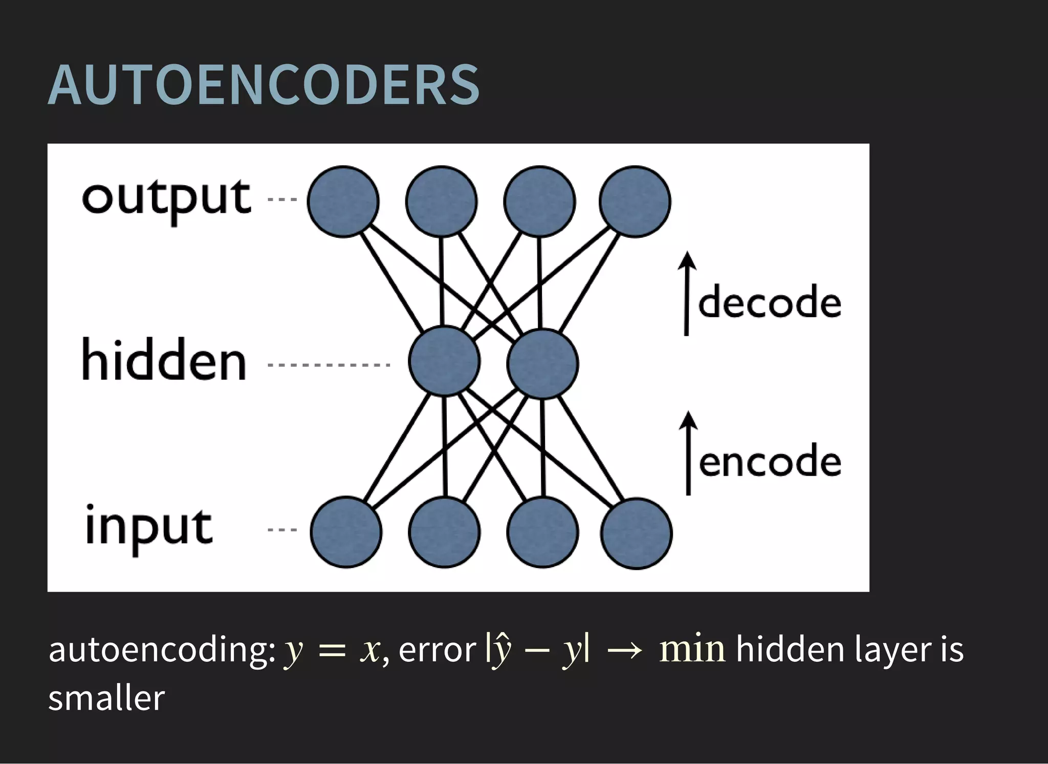
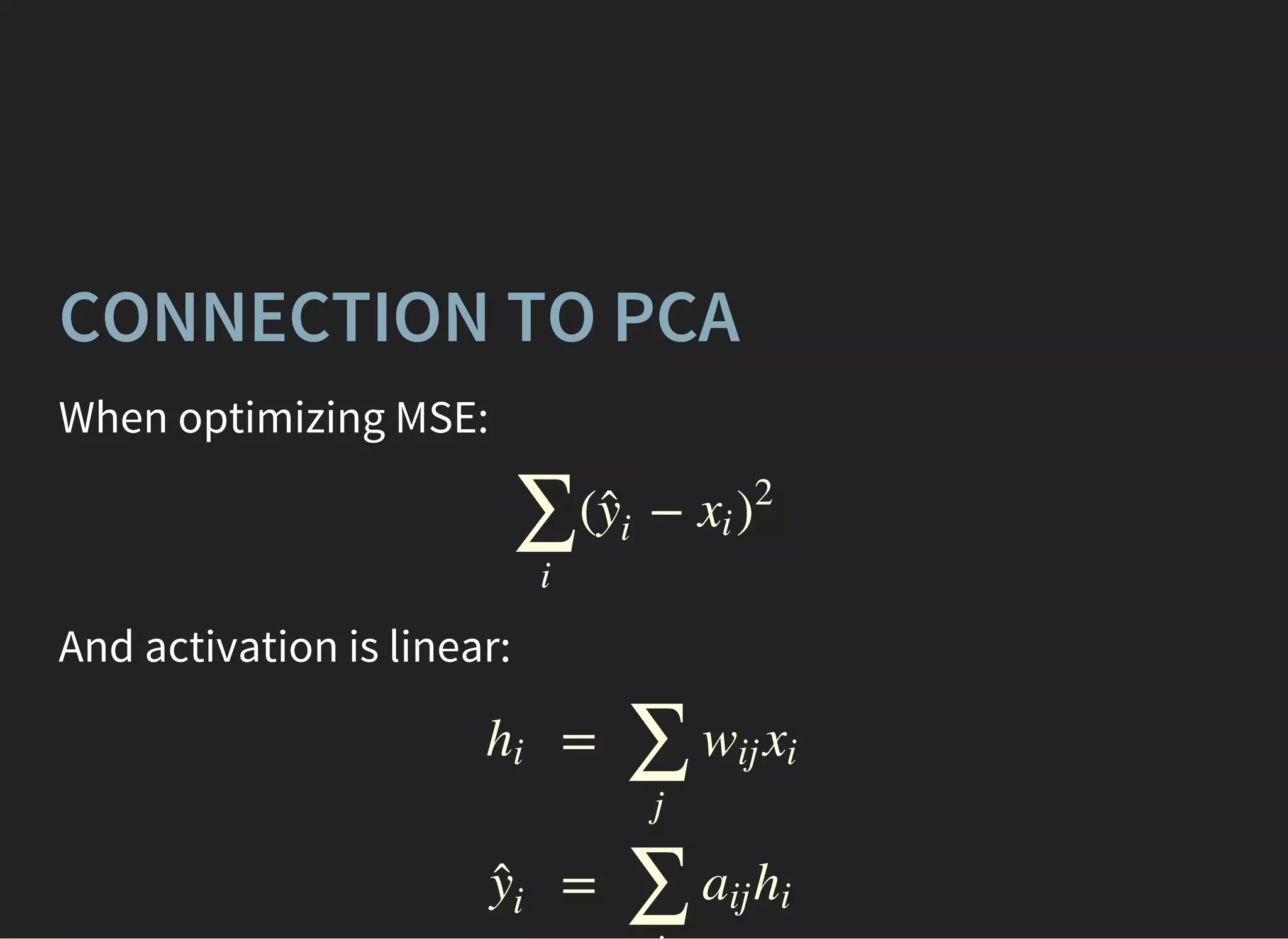
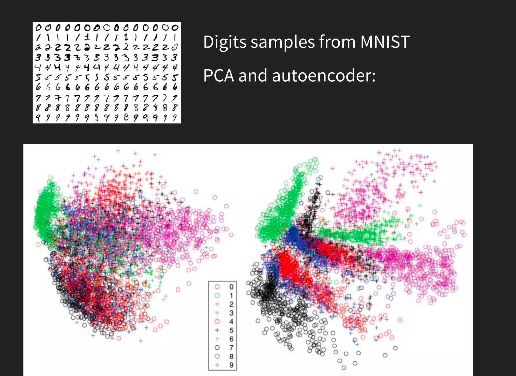
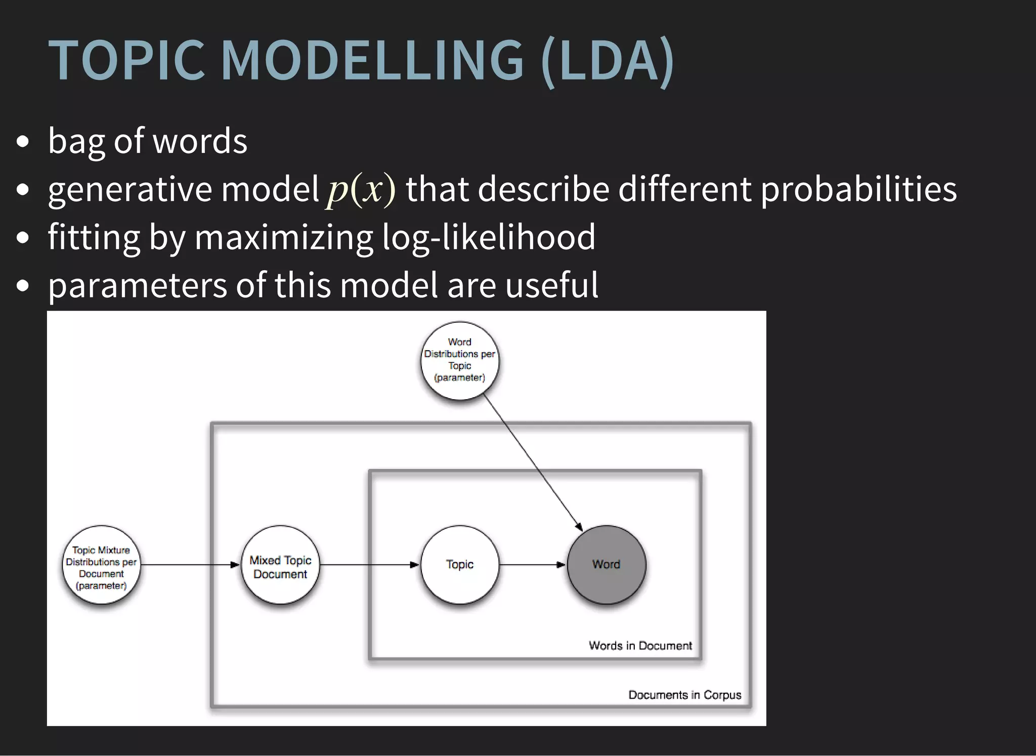
43. UNSUPERVISED LEARNING: PCA
[PEARSON, 1901]
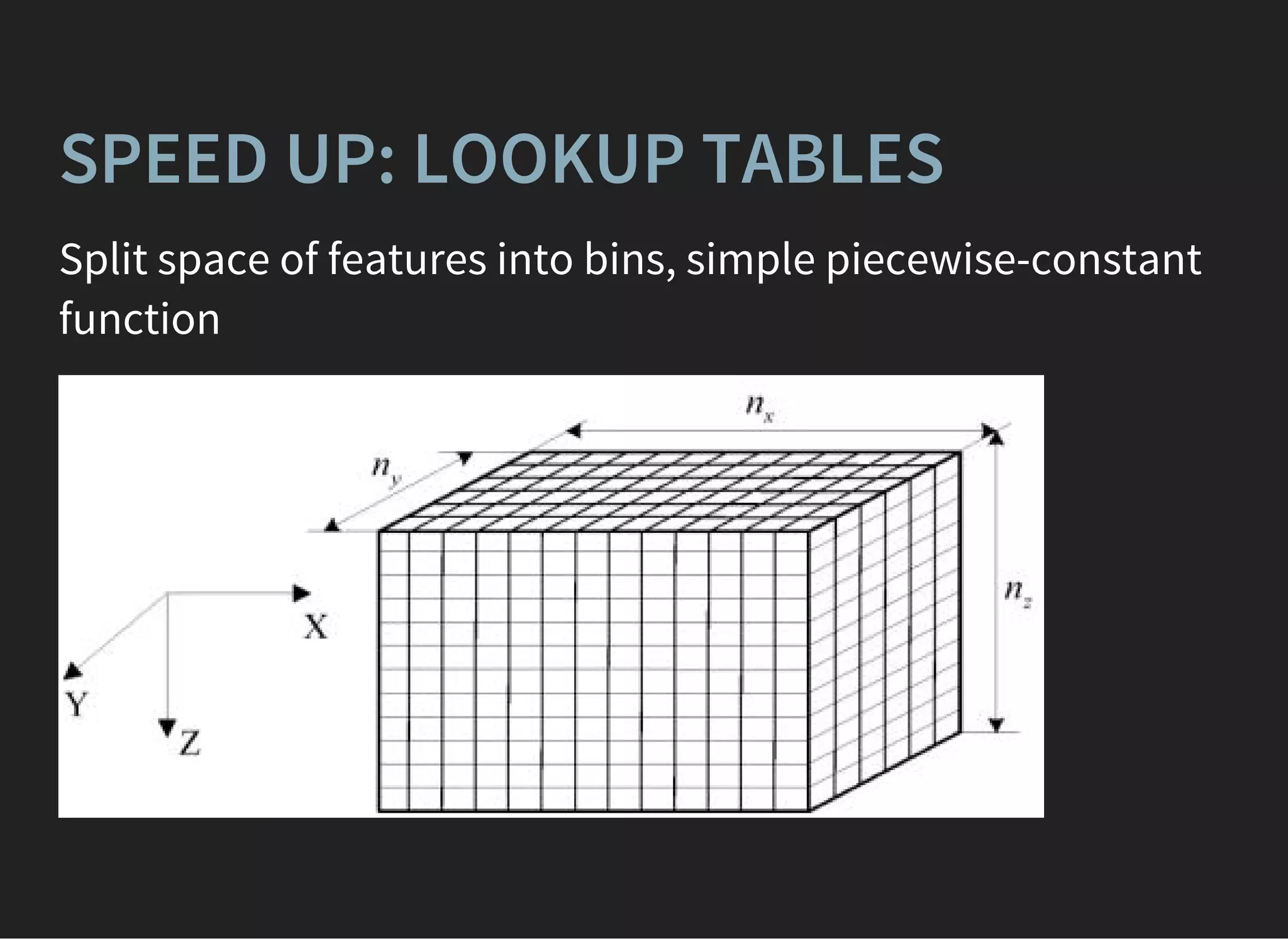
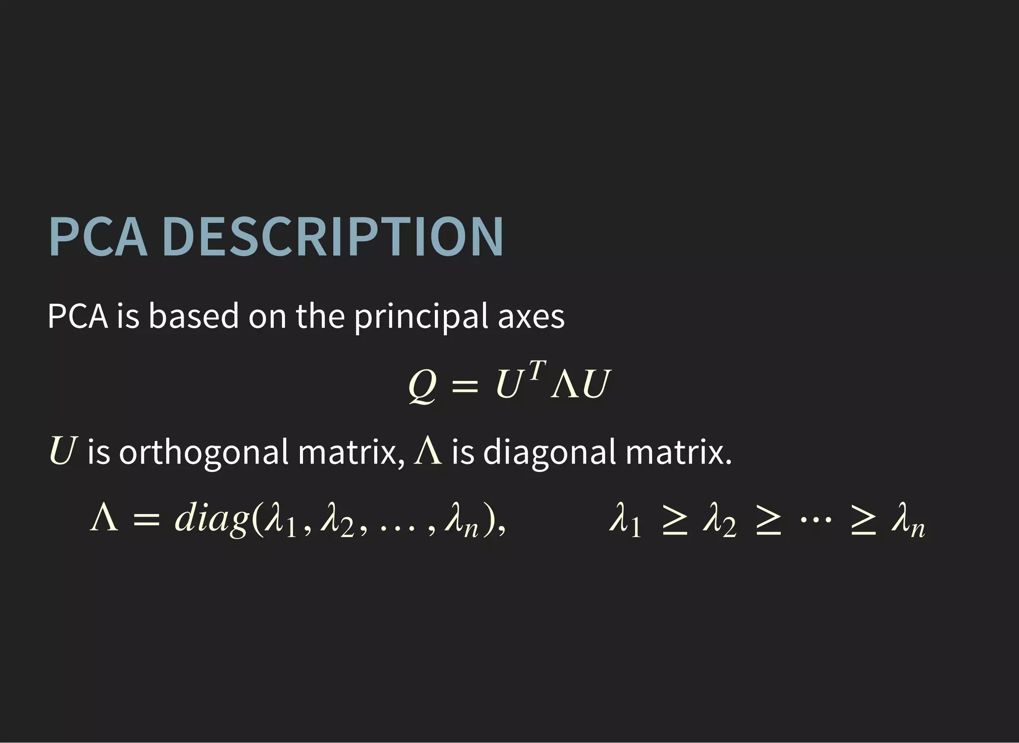
PCA is finding axes along which variation is maximal
(based on principal axis theorem)

44. PCA DESCRIPTION
PCA is based on the principal axes
is orthogonal matrix, is diagonal matrix.
Q = ΛUU
T
U Λ
Λ = diag( , , …, ), ≥ ≥ ⋯ ≥λ1 λ2 λn λ1 λ2 λn

45. PCA: EIGENFACES
Emotion = α[scared] + β[laughs] + γ[angry]+. . .

46. PCA: CALORIMETER
Electron/jet recognition in ATLAS

47. AUTOENCODERS
autoencoding: , error hidden layer is
smaller
y = x | − y| → minŷ

48. CONNECTION TO PCA
When optimizing MSE:
( −
∑
i
ŷ
i
xi )
2
And activation is linear:
hi
ŷ
i
=
=
∑
j
wij xi
∑
aij hi

49. j
Optimal solution of optimization problem is PCA.
BOTTLENECK
There is an informational bottleneck algorithm will
eager to pass the most precious information.
⇒

50. MANIFOLD LEARNING TECHNIQUES
Preserve neighbourhood/distances.

51. Digits samples from MNIST
PCA and autoencoder:

52. PART-OF-SPEECH TAGGING

53. MARKOV CHAIN

54. MARKOV CHAIN IN TEXT

55. TOPIC MODELLING (LDA)
bag of words
generative model that describe different probabilities
fitting by maximizing log-likelihood
parameters of this model are useful
p(x)

56. COLLABORATIVE RESEARCH
problem: different environments
problem: data ping-pong
solution: dedicated machine (server) for a team
restart the research = run script or notebook
!ping www.bbc.co.uk

57. REPRODUCIBLE RESEARCH
readable code
code + description + plots together
keep versions + reviews
Solution: IPython notebook + github
Example notebook
EVEN MORE REPRODUCIBILITY?
Analysis preservation: VM with all needed stuff.
Docker

58. BIRD'S EYE VIEW TO ML:
Classification
Regression
Ranking
Dimensionality reduction

59. CLUSTERING

61. DENSITY ESTIMATION

62. REPRESENTATION LEARNING
Word2vec finds representations of words.

64. THE END