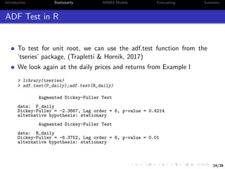
This document provides an introduction to time series analysis using R. It discusses key concepts like stationarity, unit roots, and integrated processes. It demonstrates how to check for stationarity in the SPY ETF price series and returns. Non-stationary price data can be made stationary by taking the first difference (returns). Unit root tests like the Augmented Dickey-Fuller test are used to formally test for a unit root. The document also shows how to access real-time market data using the IBrokers package in R.

1. 1/39
Introduction Stationarity ARIMA Models Forecasting Summary
Financial Time Series Analysis using R
Interactive Brokers Webinar Series
Presented by Majeed Simaan 1
1Lally School of Management at RPI
June 15, 2017

2. 2/39
Introduction Stationarity ARIMA Models Forecasting Summary
About Me
PhD Finance Candidate at RPI
Research Interests:
Banking and Risk Management
Financial Networks and Interconnectedness
Portfolio and Asset Pricing Theory
Computational and Statistical Learning
Contact:
1 simaam@rpi.edu
2 Linkedin
3 Homepage

3. 3/39
Introduction Stationarity ARIMA Models Forecasting Summary
Acknowledgment
Interactive Brokers - special thanks to
Violeta Petrova
Cynthia Tomain
Special thanks to Prof. Tom Shohfi
Faculty advisor to the RPI James Student Managed Investment
Fund
Click here for more info
Finally, special thanks to the Lally School of Management and
Technology for hosting this presentation

4. 4/39
Introduction Stationarity ARIMA Models Forecasting Summary
Agenda
Intro to R and Financial Time Series
Stationarity
ARIMA Models
Forecasting

5. 5/39
Introduction Stationarity ARIMA Models Forecasting Summary
Suggested Readings and Resources
The classic textbook on time series analysis
Hamilton, 1994
Time series using R:
1 Econometrics in R, Farnsworth, 2008
2 An introduction to analysis of financial data with R, Tsay, 2014
3 Manipulating time series in R, J. Ryan, 2017
Advanced time series using R
1 Analysis of integrated and cointegrated time series with R, Pfaff,
2008
2 Multivariate time series analysis, Tsay, 2013

6. 6/39
Introduction Stationarity ARIMA Models Forecasting Summary
Introduction

7. 7/39
Introduction Stationarity ARIMA Models Forecasting Summary
Getting Started
R
The R base system - https://cran.r-project.org/
RStudio - https://www.rstudio.com/products/rstudio/
Interactive Brokers - https://www.interactivebrokers.com
Trader Workstation (TWS)
or IB Gateway

8. 8/39
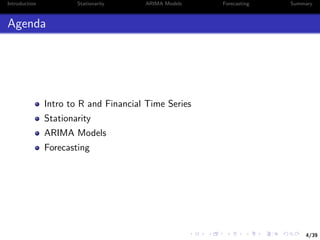
Introduction Stationarity ARIMA Models Forecasting Summary
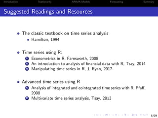
Time Series in R
The xts package, (J. A. Ryan & Ulrich, 2014), provides efficient
ways to manipulate time series1
> library(xts)
> library(lubridate)
> n <- 100
> set.seed(13)
> x <- rnorm(n)
> names(x) <- as.character(date(today()) - 0:(n-1))
> x <- as.xts(x)
> x[today(),]
[,1]
2017-06-08 0.5543269
1
lubridate package, (Grolemund & Wickham, 2011), makes date format handling much easier

9. 8/39
Introduction Stationarity ARIMA Models Forecasting Summary
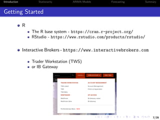
Time Series in R
The xts package, (J. A. Ryan & Ulrich, 2014), provides efficient
ways to manipulate time series1
> library(xts)
> library(lubridate)
> n <- 100
> set.seed(13)
> x <- rnorm(n)
> names(x) <- as.character(date(today()) - 0:(n-1))
> x <- as.xts(x)
> x[today(),]
[,1]
2017-06-08 0.5543269
# it is easy to plot an xts object
> plot(x)
Feb 27
2017
Mar 20
2017
Apr 10
2017
May 01
2017
May 22
2017
Jun 06
2017
−2−1012
x
1
lubridate package, (Grolemund & Wickham, 2011), makes date format handling much easier

10. 9/39
Introduction Stationarity ARIMA Models Forecasting Summary
Time Series in R II
We can also look at x as a data frame instead
> x <- data.frame(Date = date(x), x = x[,1])
> rownames(x) <- NULL
> summary(x)
Date x
Min. :2017-03-01 Min. :-2.02704
1st Qu.:2017-03-25 1st Qu.:-0.75623
Median :2017-04-19 Median :-0.07927
Mean :2017-04-19 Mean :-0.06183
3rd Qu.:2017-05-14 3rd Qu.: 0.55737
Max. :2017-06-08 Max. : 1.83616
> # add year and month variables
> x$Y <- year(x$Date); x$M <- month(x$Date);

11. 9/39
Introduction Stationarity ARIMA Models Forecasting Summary
Time Series in R II
We can also look at x as a data frame instead
> x <- data.frame(Date = date(x), x = x[,1])
> rownames(x) <- NULL
> summary(x)
Date x
Min. :2017-03-01 Min. :-2.02704
1st Qu.:2017-03-25 1st Qu.:-0.75623
Median :2017-04-19 Median :-0.07927
Mean :2017-04-19 Mean :-0.06183
3rd Qu.:2017-05-14 3rd Qu.: 0.55737
Max. :2017-06-08 Max. : 1.83616
> # add year and month variables
> x$Y <- year(x$Date); x$M <- month(x$Date);
The package plyr, (Wickham, 2011), provides efficient data split
summary
> library(plyr)
> max_month_x <- ddply(x,c("Y","M"),function(z) max(z[,"x"]))
> max_month_x # max value over month
Y M V1
1 2017 3 1.745427
2 2017 4 1.614479
3 2017 5 1.836163
4 2017 6 1.775163

12. 10/39
Introduction Stationarity ARIMA Models Forecasting Summary
IB API
The IBrokers package, J. A. Ryan, 2014, provides access to IB Trader
Workstation (TWS) API
The package also allows users to automate trades and receive real-
time data2
2
See the recent Webinar presentation by Anil Yadav here.

13. 10/39
Introduction Stationarity ARIMA Models Forecasting Summary
IB API
The IBrokers package, J. A. Ryan, 2014, provides access to IB Trader
Workstation (TWS) API
The package also allows users to automate trades and receive real-
time data2
> library(IBrokers)
> tws <- twsConnect()
> isConnected(tws) # should be true
> ac <- reqAccountUpdates(tws) # requests account details
> security <- twsSTK("SPY") # choose security of interest
> is.twsContract(security) # make sure it is identified
> P <- reqHistoricalData(tws,security, barSize = '5 mins',duration = "1 Y")
TWS Message: 2 -1 2100 API client has been unsubscribed from account data.
waiting for TWS reply on SPY .... done.
2
See the recent Webinar presentation by Anil Yadav here.

14. 10/39
Introduction Stationarity ARIMA Models Forecasting Summary
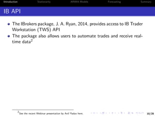
IB API
The IBrokers package, J. A. Ryan, 2014, provides access to IB Trader
Workstation (TWS) API
The package also allows users to automate trades and receive real-
time data2
> library(IBrokers)
> tws <- twsConnect()
> isConnected(tws) # should be true
> ac <- reqAccountUpdates(tws) # requests account details
> security <- twsSTK("SPY") # choose security of interest
> is.twsContract(security) # make sure it is identified
> P <- reqHistoricalData(tws,security, barSize = '5 mins',duration = "1 Y")
TWS Message: 2 -1 2100 API client has been unsubscribed from account data.
waiting for TWS reply on SPY .... done.
> P[c(1,nrow(P))] # look at first and last data points
SPY.Open SPY.High SPY.Low SPY.Close SPY.Volume SPY.WAP
2016-06-09 09:30:00 211.51 211.62 211.37 211.41 26766 211.501
2017-06-08 15:55:00 243.77 243.86 243.68 243.76 30984 243.772
SPY.hasGaps SPY.Count
2016-06-09 09:30:00 0 8378
2017-06-08 15:55:00 0 8952
2
See the recent Webinar presentation by Anil Yadav here.

15. 11/39
Introduction Stationarity ARIMA Models Forecasting Summary
Stationarity

16. 12/39
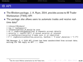
Introduction Stationarity ARIMA Models Forecasting Summary
Basic Concepts
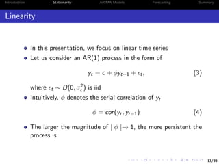
Let yt denote a time series observed over t = 1, .., T periods
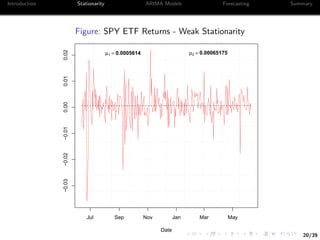
yt is called weakly stationary, if
E[yt] = µ and V[yt] = σ2
, ∀t (1)
i.e. expectation and variance of y are time invariant
3
See for instance Tsay, 2005

17. 12/39
Introduction Stationarity ARIMA Models Forecasting Summary
Basic Concepts
Let yt denote a time series observed over t = 1, .., T periods
yt is called weakly stationary, if
E[yt] = µ and V[yt] = σ2
, ∀t (1)
i.e. expectation and variance of y are time invariant
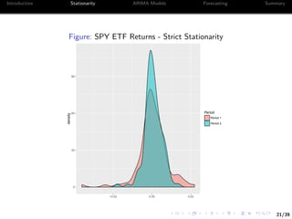
Also, yt is called strictly stationary, if
f (yt1 , ..., ytm ) = f (yt1+j , ..., ytm+j ) (2)
where m, j, and (t1, ..., tm) are arbitrary positive integers3
3
See for instance Tsay, 2005

18. 13/39
Introduction Stationarity ARIMA Models Forecasting Summary
Linearity
In this presentation, we focus on linear time series
Let us consider an AR(1) process in the form of
yt = c + φyt−1 + t, (3)
where t ∼ D(0, σ2) is iid
Intuitively, φ denotes the serial correlation of yt
φ = cor(yt, yt−1) (4)
The larger the magnitude of | φ |→ 1, the more persistent the
process is

19. 14/39
Introduction Stationarity ARIMA Models Forecasting Summary
Unit Root
Weak stationarity holds true if E[yt] = µ < ∞ for all t, such
that
µ = c + φµ ⇒ µ =
c
1 − φ
(5)
The same applies to V[yt] = σ2 < ∞, ∀t:
σ2
= φ2
σ2
+ σ2
⇒ σ2
=
σ2
1 − φ2
(6)
A necessary condition for weak stationarity implies | φ |< 1
Unit Root
If φ = 1, the process yt is a unit root

20. 15/39
Introduction Stationarity ARIMA Models Forecasting Summary
Problems with Non-Stationarity
Non-stationary data cannot be modeled or forecasted
Results based on non-stationarity can be spurious
e.g. false serial correlation in stock prices

21. 15/39
Introduction Stationarity ARIMA Models Forecasting Summary
Problems with Non-Stationarity
Non-stationary data cannot be modeled or forecasted
Results based on non-stationarity can be spurious
e.g. false serial correlation in stock prices
If yt has a unit root (non-stationary), i.e. φ = 1, with c = 0,
then
yt = yt−1 + t (7)
yt−1 = yt−2 + t−1 (8)
⇒yt =
t
s=0
s (9)
where y0 = 0
The process in (7) is unstable in nature,
the initial shock, 0, does not dissipate over time

22. 16/39
Introduction Stationarity ARIMA Models Forecasting Summary
Transformation and Integrated Process
In linear time series, transformation takes the form of a first
difference
∆yt = yt − yt−1 (10)
Taking the first difference of (7), we have
∆yt = t (11)
The process in (11) is stationary and does not depend on pre-
vious shocks

23. 16/39
Introduction Stationarity ARIMA Models Forecasting Summary
Transformation and Integrated Process
In linear time series, transformation takes the form of a first
difference
∆yt = yt − yt−1 (10)
Taking the first difference of (7), we have
∆yt = t (11)
The process in (11) is stationary and does not depend on pre-
vious shocks
Integrated Process
If yt has a unit root (non-stationary), while ∆yt = yt − yt−1 is
stationary, then yt is called integrated of first order, I(1).

24. 17/39
Introduction Stationarity ARIMA Models Forecasting Summary
Example I: SPY ETF Stationarity
Figure: SPY ETF - Violation of Weak Stationarity
Jul Sep Nov Jan Mar May
200210220230240
µ1 = 215.02
µ2 = 233.88

25. 18/39
Introduction Stationarity ARIMA Models Forecasting Summary
Figure: SPY ETF - Violation of Strict Stationarity
0.00
0.03
0.06
0.09
0.12
200 210 220 230 240
density
Period
Period 1
Period 2

26. 19/39
Introduction Stationarity ARIMA Models Forecasting Summary
Let Pt denote the price of the SPY ETF at time t and
pt = log(Pt) (12)
If pt is I(1), then ∆pt should be stationary, where
∆pt = pt − pt−1 = log
Pt
Pt−1
≈ rt (13)
denotes the return on the asset between t − 1 and t

27. 20/39
Introduction Stationarity ARIMA Models Forecasting Summary
Figure: SPY ETF Returns - Weak Stationarity
Jul Sep Nov Jan Mar May
−0.03−0.02−0.010.000.010.02
Date
µ1 = 0.0005614 µ2 = 0.00065175

28. 21/39
Introduction Stationarity ARIMA Models Forecasting Summary
Figure: SPY ETF Returns - Strict Stationarity
0
30
60
90
−0.02 0.00 0.02
density
Period
Period 1
Period 2

29. 22/39
Introduction Stationarity ARIMA Models Forecasting Summary
Let’s take a look at the serial correlation of the prices
We will focus on the closing price
> find.close <- grep("Close",names(P))
> P_daily <- apply.daily(P[,find.close],function(x) x[nrow(x),])
> dim(P_daily)
[1] 252 1
> cor(P_daily[-1],lag(P_daily)[-1])
SPY.Close
SPY.Close 0.99238

30. 22/39
Introduction Stationarity ARIMA Models Forecasting Summary
Let’s take a look at the serial correlation of the prices
We will focus on the closing price
> find.close <- grep("Close",names(P))
> P_daily <- apply.daily(P[,find.close],function(x) x[nrow(x),])
> dim(P_daily)
[1] 252 1
> cor(P_daily[-1],lag(P_daily)[-1])
SPY.Close
SPY.Close 0.99238
On the other hand, the corresponding statistic for returns is
> R_daily <- P_daily[-1]/lag(P_daily)[-1] - 1
> cor(R_daily[-1],lag(R_daily)[-1])
SPY.Close
SPY.Close -0.06828564

31. 23/39
Introduction Stationarity ARIMA Models Forecasting Summary
Test for Unit Root
It is important to plot the time series before running any tests
of unit root
It is recommended to use reasoning where the non-stationarity
might come from
In the case of stock prices, time is one major factor
Assuming that a time series has a unit root when it does not
can bias inference

32. 23/39
Introduction Stationarity ARIMA Models Forecasting Summary
Test for Unit Root
It is important to plot the time series before running any tests
of unit root
It is recommended to use reasoning where the non-stationarity
might come from
In the case of stock prices, time is one major factor
Assuming that a time series has a unit root when it does not
can bias inference
Augmented Dickey-Fuller Test
A common test for unit root is the Augmented Dickey-Fuller
(ADF) test
It tests the null hypothesis whether a unit root is present in the
time series
The more negative the statistic is the more likely to reject the
null

33. 24/39
Introduction Stationarity ARIMA Models Forecasting Summary
ADF Test in R
To test for unit root, we can use the adf.test function from the
’tseries’ package, (Trapletti & Hornik, 2017)
We look again at the daily prices and returns from Example I
> library(tseries)
> adf.test(P_daily);adf.test(R_daily)
Augmented Dickey-Fuller Test
data: P_daily
Dickey-Fuller = -2.3667, Lag order = 6, p-value = 0.4214
alternative hypothesis: stationary
Augmented Dickey-Fuller Test
data: R_daily
Dickey-Fuller = -6.3752, Lag order = 6, p-value = 0.01
alternative hypothesis: stationary

34. 25/39
Introduction Stationarity ARIMA Models Forecasting Summary
ARIMA Models
(Autoregressive Integrated Moving Average)

35. 26/39
Introduction Stationarity ARIMA Models Forecasting Summary
ARIMA Models
Let yt follow an ARIMA(p, d, q) model, where
1 p is the order of autoregressive (AR) model
2 d is the order of differencing to yield a I(0) process
3 q is the order of the moving average (MA) model

36. 26/39
Introduction Stationarity ARIMA Models Forecasting Summary
ARIMA Models
Let yt follow an ARIMA(p, d, q) model, where
1 p is the order of autoregressive (AR) model
2 d is the order of differencing to yield a I(0) process
3 q is the order of the moving average (MA) model
For instance,
AR(p) = ARIMA(p, 0, 0) (14)
MA(q) = ARIMA(0, 0, q) (15)

37. 26/39
Introduction Stationarity ARIMA Models Forecasting Summary
ARIMA Models
Let yt follow an ARIMA(p, d, q) model, where
1 p is the order of autoregressive (AR) model
2 d is the order of differencing to yield a I(0) process
3 q is the order of the moving average (MA) model
For instance,
AR(p) = ARIMA(p, 0, 0) (14)
MA(q) = ARIMA(0, 0, q) (15)
Special Case
If yt has a unit root, i.e. I(1) , then first difference, ∆yt, yields
a stationary process
Also, if ∆yt follows an AR(1) process, then we conclude that
yt has an ARIMA(1, 1, 0) process

38. 27/39
Introduction Stationarity ARIMA Models Forecasting Summary
ARIMA Identification
Identification of ARIMA can be facilitated as follows
1 Find the order of integration I(d) of the time series
e.g. most stock prices are integrated of order 1, d = 1
2 Look at indicators in the data for AR and MA orders
A common approach is to refer to the PACF and ACF, respec-
tively4
3 Consider an information criteria, e.g. AIC (Sakamoto, Ishiguro,
& Kitagawa, 1986)
4 Finally, test whether the residuals of the identified model follow
a white noise process
4
See this discussion for further reading.

39. 27/39
Introduction Stationarity ARIMA Models Forecasting Summary
ARIMA Identification
Identification of ARIMA can be facilitated as follows
1 Find the order of integration I(d) of the time series
e.g. most stock prices are integrated of order 1, d = 1
2 Look at indicators in the data for AR and MA orders
A common approach is to refer to the PACF and ACF, respec-
tively4
3 Consider an information criteria, e.g. AIC (Sakamoto et al.,
1986)
4 Finally, test whether the residuals of the identified model follow
a white noise process
Ljung-Box Statistic
This statistic is useful to test whether residuals are serially cor-
related
A value around zero (large p.value) implies a good fit
4
See this discussion for further reading.

40. 28/39
Introduction Stationarity ARIMA Models Forecasting Summary
Example II: Identifying ARIMA Models
We consider a simulated time series from a given ARIMA model
Specifically, we consider an ARIMA(3,1,2) process
> N <- 10^3
> set.seed(13)
> y <- arima.sim(N,model = list(order = c(3,1,2), ar = c(0.8, -0.5,0.4),
+ ma = c(0.5,-0.3))) + 200
# Note that y is a ts object rather than xts
Step 1: Plot and Test for Unit Root
> plot(y);
> ADF <- adf.test(y); ADF$p.value
[1] 0.4148301
# lag on ts object should be assigned as -1
> delta_y <- na.omit(y - lag(y,-1) )
> plot(delta_y);
> ADF2 <- adf.test(delta_y); ADF2$p.value
[1] 0.01

41. 29/39
Introduction Stationarity ARIMA Models Forecasting Summary
Step 1 tells us that d = 1, i.e. yt follows an ARIMA(p, 1, q)
We need to identify p and q
Step 2: Identify p and q using the AIC information criterion
> p.seq <- 0:4
> q.seq <- 0:4
> pq.seq <- expand.grid(p.seq,q.seq)
> AIC.list <- lapply(1:nrow(pq.seq),function(i)
+ AIC(arima(y,c(pq.seq[i,1],1,pq.seq[i,2]))))
> AIC.matrix <- matrix(unlist(AIC.list),length(p.seq))
> rownames(AIC.matrix) <- p.seq
> colnames(AIC.matrix) <- q.seq
AIC.matrix
p q 0 1 2 3 4
0 3973.32 3075.67 2923.06 2914.88 2916.86
1 3542.07 2983.22 2916.50 2916.88 2883.02
2 3407.54 2949.70 2912.02 2907.37 2866.26
3 3053.10 2851.96 2844.42 2846.41 2848.31
4 2987.36 2845.46 2846.41 2847.81 2850.41

42. 30/39
Introduction Stationarity ARIMA Models Forecasting Summary
It follows from Step 2 that the optimal combination is (p = 3, q = 2)
Alternatively, we can use the auto.arima function
> identify.arima <- auto.arima(y)
> identify.arima
Series: y
ARIMA(3,1,2)
Coefficients:
ar1 ar2 ar3 ma1 ma2
0.7758 -0.4821 0.3875 0.5376 -0.2752
s.e. 0.0785 0.0448 0.0315 0.0836 0.0796
sigma^2 estimated as 0.9965: log likelihood=-1416.21
AIC=2844.42 AICc=2844.5 BIC=2873.87
In either case, we get consistent results indicating that the model is
ARIMA(3,1,2)

43. 31/39
Introduction Stationarity ARIMA Models Forecasting Summary
Finally, we look at the residuals of the fitted model
Step 3: check residuals
> Box.test(residuals(identify.arima),type = "Ljung-Box")
Box-Ljung test
data: residuals(identify.arima)
X-squared = 0.00087004, df = 1, p-value = 0.9765
> library(forecast)
> Acf(residuals(identify.arima),main = "")
−0.10−0.050.000.050.10
Lag
ACF
0 5 10 15 20 25 30

44. 32/39
Introduction Stationarity ARIMA Models Forecasting Summary
Forecasting

45. 33/39
Introduction Stationarity ARIMA Models Forecasting Summary
Forecasting
So far, we learned how to identify a time series model
For application, we are interested in forecasting future values
of the time series
Such decision will be based on a history of T periods
T periods to fit the model
and a number of lags to serve as forecast inputs
Hence, our decision will be based on the quality of
1 the data
2 the fitted model

46. 34/39
Introduction Stationarity ARIMA Models Forecasting Summary
Rolling Window
We will use a rolling window approach to perform and evaluate
forecasts
Set t = 150 and perform the following steps
1 Standing at the end of day t
2 Use T = 150 historic days of data (including day t) to fit an
ARIMA model
3 Make a forecast for next period, i.e. t + 1
4 Set t → t + 1 and go back to Step 1
The above steps are repeated until t + 1 becomes the last ob-
servation in the time series

47. 35/39
Introduction Stationarity ARIMA Models Forecasting Summary
Example III: Forecast the SPY ETF
In total we have 252 days of closing prices for the SPY ETF
To avoid price non-stationary, we focus on returns alone
This leaves us with 101 days to test our forecasts5
We consider three models for forecast
1 Dynamically fitted ARIMA(p,0,q) model
2 Dynamically fitted AR(1) model
3 Plain moving average (momentum)
> library(forecast)
> T. <- 150
> arma.list <- numeric()
> ar1.list <- numeric()
> ma.list <- numeric()
> for(i in T.:(length(R_daily)-1) ) {
+ arma.list[i] <- list(auto.arima(R_daily[(i-T.+1):i])) # ARIMA(p,0,q)
+ ar1.list[i] <- list(arima(R_daily[(i-T.+1):i],c(1,0,0))) # AR(1)
+ ma.list[i] <- list(mean(R_daily[(i-T.+1):i])) # momentum
+ }
5
The experiment relies on the forecast package, Hyndman, 2017

48. 36/39
Introduction Stationarity ARIMA Models Forecasting Summary
> y_hat <- sapply(arma.list[T.:length(arma.list)],
+ function(x) forecast(x,1)[[4]] )
> y_hat2 <- sapply(ar1.list[T.:length(ar1.list)],
+ function(x) forecast(x,1)[[4]] )
> y_hat3 <- sign(unlist(ma.list))
> forecast_accuracy <- cbind(mean(sign(y_hat) == sign(y)),
+ mean(sign(y_hat2) == sign(y)),
+ mean(sign(y_hat3) == sign(y)))
Finally, summarize the forecast accuracy in a table
ARIMA AR(1) Momentum
Accuracy 55.45% 53.47% 52.48%
Among the three, ARIMA performs the best
Could be attributed to more flexibility in fitting the model over time

49. 37/39
Introduction Stationarity ARIMA Models Forecasting Summary
While AR(1) is a constrained ARIMA model, note that the autore-
gressive coefficient still changes dramatically over time
Red line denotes the SPY ETF daily return
Black line denotes the estimated AR(1) coefficient over time, i.e. φ
Jan 13
2017
Feb 06
2017
Feb 27
2017
Mar 20
2017
Apr 10
2017
May 01
2017
May 22
2017
−0.15−0.10−0.050.00
φ
rt

50. 38/39
Introduction Stationarity ARIMA Models Forecasting Summary
Summary
Importance of stationarity
Non-stationary models could imply spurious results
Plots are always insightful
Use tests carefully
Consider multiple time series to form forecasts
Hence the idea of multivariate time series analysis

51. 39/39
Introduction Stationarity ARIMA Models Forecasting Summary
Good Luck!

52. 40/39
References
References I
[]Farnsworth, G. V. 2008. Econometrics in r. Technical
report, October 2008. Available at http://cran. rproject.
org/doc/contrib/Farnsworth-EconometricsInR. pdf.
[]Grolemund, G., & Wickham, H. 2011. Dates and times made easy
with lubridate. Journal of Statistical Software, 40(3), 1–25.
Retrieved from http://www.jstatsoft.org/v40/i03/
[]Hamilton, J. D. 1994. Time series analysis (Vol. 2). Princeton
university press Princeton.
[]Hyndman, R. J. 2017. forecast: Forecasting functions for time
series and linear models [Computer software manual]. Re-
trieved from http://github.com/robjhyndman/forecast
(R package version 8.0)
[]Pfaff, B. 2008. Analysis of integrated and cointegrated time series
with r. Springer Science & Business Media.

53. 41/39
References
References II
[]Ryan, J. 2017. Manipulating time series data in r with xts & zoo.
Data Camp.
[]Ryan, J. A. 2014. Ibrokers: R api to interactive brokers trader
workstation [Computer software manual]. Retrieved from
https://CRAN.R-project.org/package=IBrokers (R
package version 0.9-12)
[]Ryan, J. A., & Ulrich, J. M. 2014. xts: extensible time series
[Computer software manual]. Retrieved from https://CRAN
.R-project.org/package=xts (R package version 0.9-7)
[]Sakamoto, Y., Ishiguro, M., & Kitagawa, G. 1986. Akaike infor-
mation criterion statistics. Dordrecht, The Netherlands: D.
Reidel.
[]Trapletti, A., & Hornik, K. 2017. tseries: Time series analy-
sis and computational finance [Computer software manual].
Retrieved from https://CRAN.R-project.org/package=
tseries (R package version 0.10-41.)

54. 42/39
References
References III
[]Tsay, R. S. 2005. Analysis of financial time series (Vol. 543). John
Wiley & Sons.
[]Tsay, R. S. 2013. Multivariate time series analysis: with r and
financial applications. John Wiley & Sons.
[]Tsay, R. S. 2014. An introduction to analysis of financial data
with r. John Wiley & Sons.
[]Wickham, H. 2011. The split-apply-combine strategy for data anal-
ysis. Journal of Statistical Software, 40(1), 1–29. Retrieved
from http://www.jstatsoft.org/v40/i01/