Download to read offline

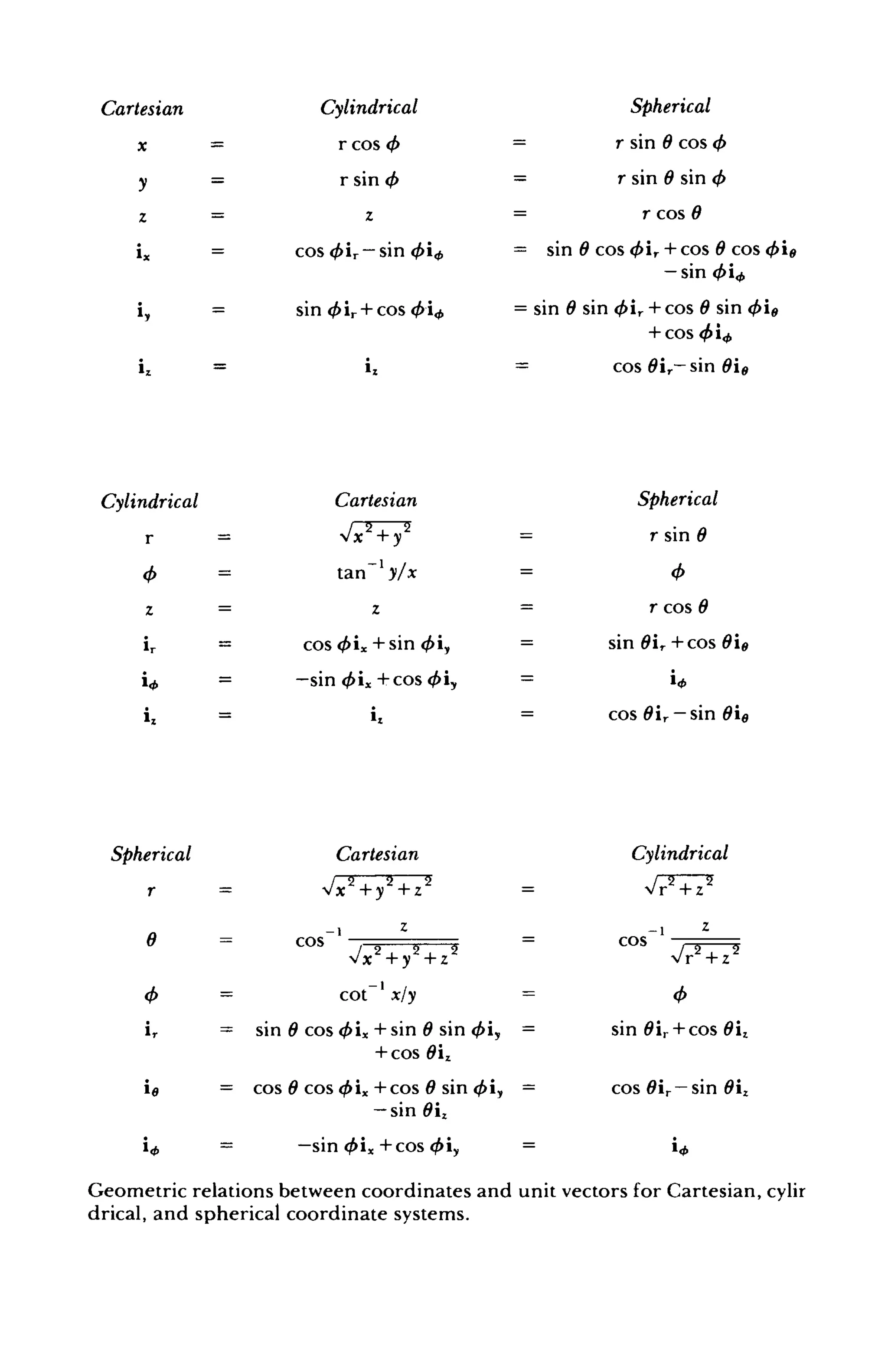
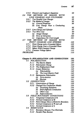
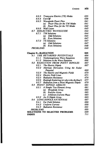
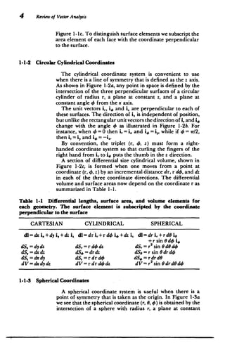
![CartesianCoordinates(x, y, z)
Vf = Ofi.+Ofi,+Ofi.
ax ay Oz
+-A=,++-i
V- aA,, aA, aA, 2
ax ay az
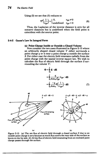
aA aA)
VxA ay_ a (aA
,(- _)+i
=i. (LAI )+ _8A -(
ay az ) az a.x) ay
2
f
V2f+!L+f+a
Ox2 j Z
CylindricalCoordinates (r, 4, z)
Of. 1 Of. Of
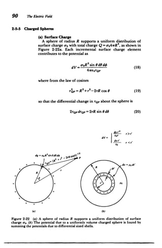
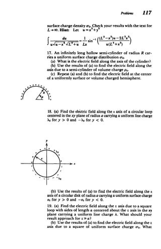
Vf= r+ i,+ iz
+A MA.
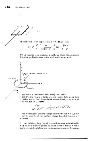
V -A= Ia(rA,.)+ -.
r Or r ao az
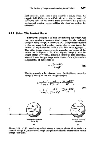
VxA=i - +ixaz Or + OA r a4
0/f a Of 1a2f a2f
V'f= r +
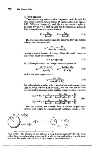
+
42
r Or On) r O
SphericalCoordinates (r, 0, 4,)
Vf=i,.+ afi+
Or r aO r sin 0 a4
V A = (r2A,)+ 1 (sin OA.) 1 oA*
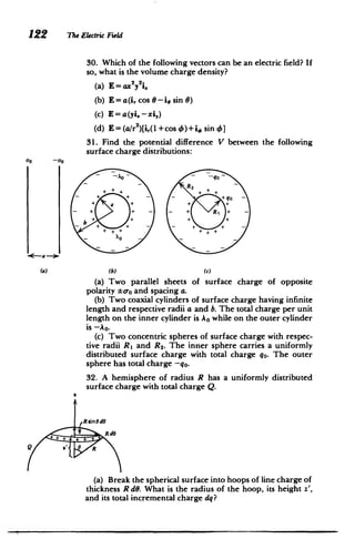
r2 ar r sin 0 aI r sin 0 a4
VxA=i1 a(sin OAs) aA.
'r sineL 80 a4
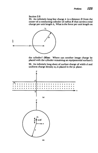
I rIAM, a(rA) 1 [a(rA#) OA,.
r sin{ 0r] rL Or aeJ
2
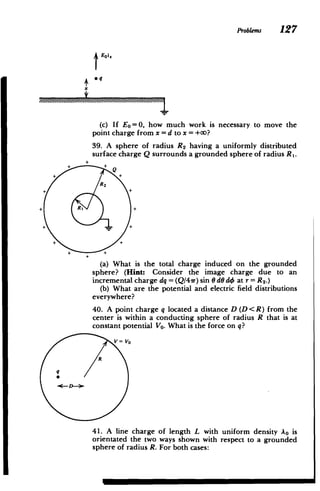
f
V f = r + r s n sin0 ) +Of I a
rf ar' Or. r- -s i n aG ai r sin 04, 0](https://image.slidesharecdn.com/mitres6002s08part1-211102045902/85/Mitres-6-002_s08_part1-3-320.jpg)
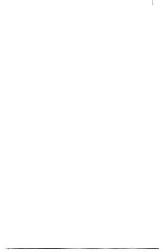
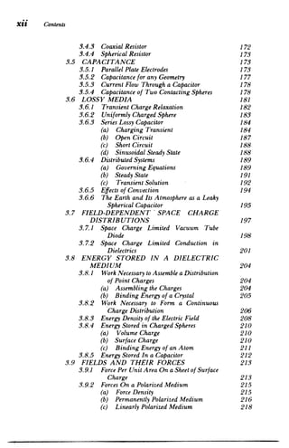
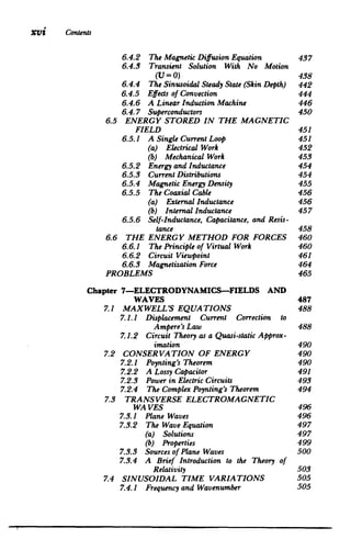
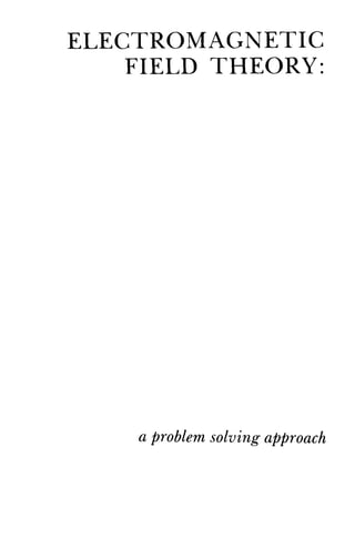
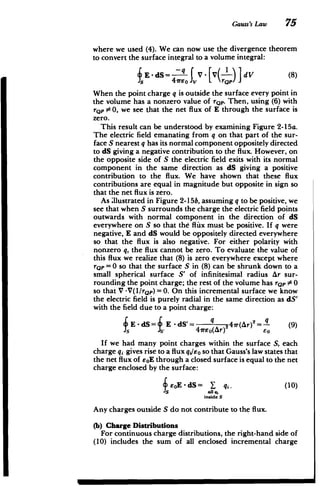
![MAXWELL'S EQUATIONS
Integral Differential Boundary Conditions
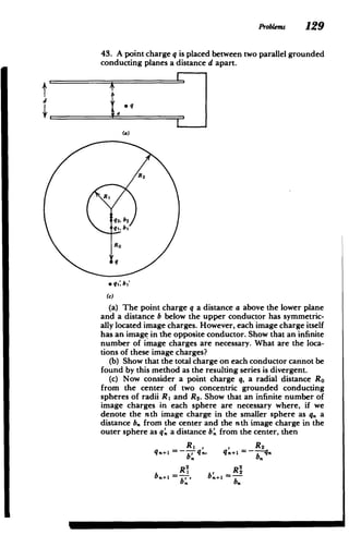
Faraday's Law
d C B
E'-dl=-- B-dS VxE=- nx(E'-E')=0.
dtJI at
Ampere's Law with Maxwell's Displacement Current Correction
H-dl= Jf,-dS VXH=Jf+aD nX(H 2 -H 1 )=Kf
+ D-dS
~it-s
Gauss's Law
V - D=p n - (D2 -D 1)= o-
D'-dS=t pfdV
B-dS=0 V-B=0
Conservation of Charge
J,- dS+ pfdV=O V-J,+ =0 n - (J2-J)+" 0
sVd at a
Usual Linear Constitutive Laws
D=eE
B= H
Jf= o-(E+vX B)= a-E' [Ohm's law for moving media with velocity v]
PHYSICAL CONSTANTS
Constant Symbol Value units
Speed of light in vacuum c 2.9979 x 10 8
= 3 x 10⁸ m/sec
Elementary electron charge e 1.602 x 10~'9 coul
Electron rest mass M, 9.11 x 10 3
kg
Electron charge to mass ratio e 1.76 x 10" coul/kg
M,
Proton rest mass I, 1.67 x 10⁻²⁷ kg
Boltzmann constant k 1.38 x 10⁻²³ joule/*K
Gravitation constant G 6.67 x 10-" nt-m2
/(kg) 2
Acceleration of gravity g 9.807 m/(sec)2
10
*
Permittivity of free space 60 8.854 x 10~2~36r farad/m
Permeability of free space A0 4r X 10 henry/m
Planck's constant h 6.6256 x 10⁻³⁴ joule-sec
Impedance of free space i1o 4 376.73- 120ir ohms
Avogadro's number Ar 6.023 x 10²³ atoms/mole](https://image.slidesharecdn.com/mitres6002s08part1-211102045902/85/Mitres-6-002_s08_part1-5-320.jpg)

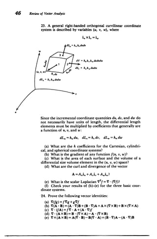
![CONTENTS
Chapter 1-REVIEW OF VECTOR ANALYSIS
1.1 COORDINATE SYSTEMS
1.1.1 Rectangular(Cartesian)Coordinates
1.1.2 CircularCylindricalCoordinates
1.1.3 SphericalCoordinates
1.2 VECTOR ALGEBRA
1.2.1 Scalarsand Vectors
1.2.2 Multiplicationof a Vector by aScalar
1.2.3 Addition and Subtraction
1.2.4 The Dot (Scalar)Product
1.2.5 The Cross(Vector) Product
1.3 THE GRADIENT AND THE DEL
OPERATOR
1.3.1 The Gradient
1.3.2 CurvilinearCoordinates
(a) Cylindrical
(b) Spherical
1.3.3 The Line Integral
1.4 FLUX AND DIVERGENCE
1.4.1 Flux
1.4.2 Divergence
1.4.3 CurvilinearCoordinates
(a) CylindricalCoordinates
(b) SphericalCoordinates
1.4.4 The Divergence Theorem
1.5 THE CURL AND STOKES' THEOREM
1.5.1 Curl
1.5.2 The Curlfor CurvilinearCoordinates
(a) CylindricalCoordinates
(b) SphericalCoordinates
1.5.3 Stokes' Theorem
1.5.4 Some Useful Vector Relations
(a) The Curl of the Gradient is Zero
IV x(Vf)=O]
(b) The Divergence of the Curl is Zero
[V - (V X A)= 0
PROBLEMS
Chapter 2-THE ELECTRIC FIELD
2.1 ELECTRIC CHARGE
2.1.1 Chargingby Contact
2.1.2 ElectrostaticInduction
2.1.3 Faraday's"Ice-Pail"Experiment
2.2 THE COULOMB FORCE LAW
BETWEEN STATIONARY CHARGES
2.2.1 Coulomb'sLaw
ix](https://image.slidesharecdn.com/mitres6002s08part1-211102045902/85/Mitres-6-002_s08_part1-15-320.jpg)


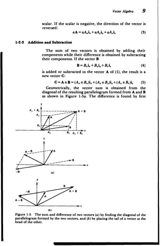
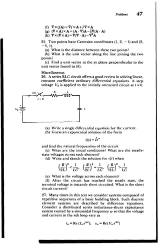
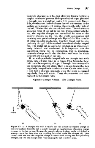
![8 Review of Vector Analysis
being especially important in our future study. Vectors, such
as velocity and force, must-also have their direction specified
and in this text are printed in boldface type. They are
completely described by their components along three coor
dinate directions as shown for rectangular coordinates in
Figure 1-4. A vector is represented by a directed line segment
in the direction of the vector with its length proportional to its
magnitude. The vector
A = A.i. +A~i,+Ai. (1)
in Figure 1-4 has magnitude
A =JAI =[A i+A' +A, ]"' (2)
Note that each of the components in (1) (A., A,, and A.) are
themselves scalars. The direction of each of the components
is given by the unit vectors. We could describe a vector in any
of the coordinate systems replacing the subscripts (x, y, z) by
(r, 0, z) or (r, 0, 4); however, for conciseness we often use
rectangular coordinates for general discussion.
1-2-2 Multiplication of a Vector by a Scalar
If a vector is multiplied by a positive scalar, its direction
remains unchanged but its magnitude is multiplied by the
Al
A
|t
I
I
I
I
I
A
Figure 1-4
directions.
A = At i,+ Ayiy+ Ai,
A I= A = {A2 +A 2 + A.2
A vector is described by its components along the three coordinate](https://image.slidesharecdn.com/mitres6002s08part1-211102045902/85/Mitres-6-002_s08_part1-36-320.jpg)
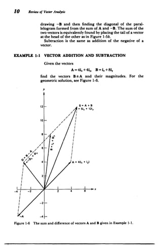
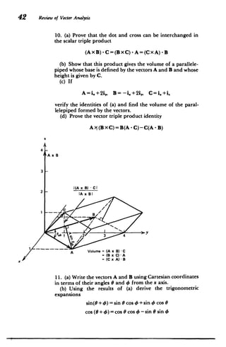
![Vector Algebra II
SOLUTION
Sum
S= A +B = (4+1)i, +(4+8)i, = 5i, + 12i,
S=[5 2+12]12= 13
Difference
D= B-A = (1 -4)i, +(8-4)i, = -3, +4i,
D = [(-3) 2+42 ]1 = 5
1-2-4 The Dot (Scalar) Product
The dot product between two vectors results in a scalar and
is defined as
A - B=AB cos 0 (6)
where 0 is the smaller angle between the two vectors. The
term A cos 0 is the component of the vector A in the direction
of B shown in Figure 1-7. One application of the dot product
arises in computing the incremental work dW necessary to
move an object a differential vector distance dl by a force F.
Only the component of force in the direction of displacement
contributes to the work
dW=F-dl (7)
The dot product has maximum value when the two vectors
are colinear (0 =0) so that the dot product of a vector with
itself is just the square of its magnitude. The dot product is
zero if the vectors are perpendicular (0 = 7r/2). These prop
erties mean that the dot product between different orthog
onal unit vectors at the same point is zero, while the dot
Y A
B
A B=AB cos 0
COsa
Figure 1-7 The dot product between two vectors.](https://image.slidesharecdn.com/mitres6002s08part1-211102045902/85/Mitres-6-002_s08_part1-39-320.jpg)
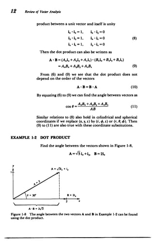
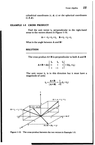
![Vector Algebra 13
SOLUTION
From (11)
cos8= =
A,+A'] B. 2
0 = cos-I -= 30*
2
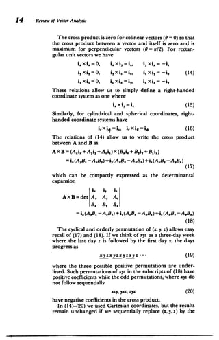
1-2-5 The Cross (Vector) Product
The cross product between two vectors A x B is defined as a
vector perpendicular to both A and B, which is in the direc
tion of the thumb when using the right-hand rule of curling
the fingers of the right hand from A to B as shown in Figure
1-9. The magnitude of the cross product is
JAXB =AB sin 6 (12)
where 0 is the enclosed angle between A and B. Geometric
ally, (12) gives the area of the parallelogram formed with A
and B as adjacent sides. Interchanging the order of A and B
reverses the sign of the cross product:
AXB= -BXA (13)
A x 8
A
AS
A
Positive
0 sense
from A to B
B x A = -A x B
(a) (b)
Figure 1-9 (a) The cross product between two vectors results in a vector perpendic
ular to both vectors in the direction given by the right-hand rule. (b) Changing the
order of vectors in the cross product reverses the direction of the resultant vector.](https://image.slidesharecdn.com/mitres6002s08part1-211102045902/85/Mitres-6-002_s08_part1-41-320.jpg)
![24 Review of Vector Analysis
multiplications of the component of A perpendicular to the
surface and the surface area. The flux then reduces to the form
+ [A,(y +Ay)-A,(y)]
D(A.(x)-Ax(x-Ax)]
AX Ay
+[A. (z + Az) -A. (z)]A yA 3
+Ax Ay Az (3)
AZ
We have written (3) in this form so that in the limit as the
volume becomes infinitesimally small, each of the bracketed
terms defines a partial derivative
(A, 3A, Az
lim (D= + + V (4)
Ax-O ax ayaz
where AV = Ax Ay Az is the volume enclosed by the surface S.
The coefficient of AV in (4) is a scalar and is called the
divergence of A. It can be recognized as the dot product
between the vector del operator of Section 1-3-1 and the
vector A:
aAx 8,A, aA,
div A = V -A =--+ + (5)
ax ay az
1-4-3 Curvilinear Coordinates
In cylindrical and spherical coordinates, the divergence
operation is not simply the dot product between a vector and
the del operator because the directions of the unit vectors are
a function of the coordinates. Thus, derivatives of the unit
vectors have nonzero contributions. It is easiest to use the
generalized definition of the divergence independent of the
coordinate system, obtained from (1)-(5) as
V- A= lim J5A-dS (6)
AV-0o AV
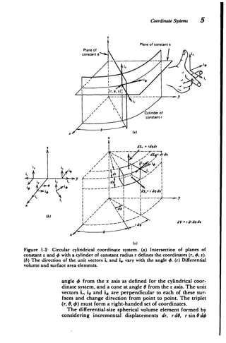
(a) Cylindrical Coordinates
In cylindrical coordinates we use the small volume shown in
Figure 1-16a to evaluate the net flux as
= A - dS =f (r+Ar)A , dO dz - rArir d dz
+ I A dr dz - f A dr dz
J"
" fj rA,,I+A, dr doS - rA,,,drdo (7)](https://image.slidesharecdn.com/mitres6002s08part1-211102045902/85/Mitres-6-002_s08_part1-52-320.jpg)
![x
Flux and Divergence 25
S
dS, = r dr do
dS, = dr ds
As
dS, =V( + Ar) do As
(a)
dS = (r + Ar)2
sin 0 dO do
= r dr dO
) <dSd
3
o2
7' = r sin(O + AO) dr do
x/
(b)
Figure 1-16 Infinitesimal volumes used to define the divergence of a vector in
(a) cylindrical and (b) spherical geometries.
r 7r
Again, because the volume is small, we can treat it as approx
imately rectangular with the components of A approximately
constant along each face. Then factoring out the volume
A V =rAr AO Az in (7),
I [(r + Ar)A,,,-rA
,
[I A ] [A -A. rAr 4 Az (8)
r AO Az
M M](https://image.slidesharecdn.com/mitres6002s08part1-211102045902/85/Mitres-6-002_s08_part1-53-320.jpg)
![26 Review of Vector Analysis
lets each of the bracketed terms become a partial derivative as
the differential lengths approach zero and (8) becomes an
exact relation. The divergence is then
* s
A-dS 1 8 1BA, 8A.
V -A= lim -= (rA,)+I +- (9)
A,+o A V rOr r a4 8z
(b) Spherical Coordinates
Similar operations on the spherical volume element AV=
r2
sin 0 Ar AO A4 in Figure 1-16b defines the net flux through
the surfaces:
4= A -dS
[(r + &r)2
Ar,+, - r2
A,,]
r2 Ar
[AA,, sin (0 +A#)-Ae,, sin 8]
r sin 8 AG
+ [A... A1.r 2
sin OAr AOAO (10)
The divergence in spherical coordinates is then
5 A -dS
V- A= lim
Ar-.O AV
=- - (r'A,) + .1 8
-(Ae 1 BA, (1
sin 0) + -- (11)
r ar r sin 80 r sinG ao
1-4-4 The Divergence Theorem
If we now take many adjoining incremental volumes of any
shape, we form a macroscopic volume V with enclosing sur
face S as shown in Figure 1-17a. However, each interior
common surface between incremental volumes has the flux
leaving one volume (positive flux contribution) just entering
the adjacent volume (negative flux contribution) as in Figure
1-17b. The net contribution to the flux for the surface integral
of (1) is zero for all interior surfaces. Nonzero contributions
to the flux are obtained only for those surfaces which bound
the outer surface S of V. Although the surface contributions
to the flux using (1) cancel for all interior volumes, the flux
obtained from (4) in terms of the divergence operation for](https://image.slidesharecdn.com/mitres6002s08part1-211102045902/85/Mitres-6-002_s08_part1-54-320.jpg)
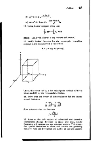
![The Curl and Stokes' .Theorem 29
around a closed path called the circulation:
C= A - dl (1)
where if C is the work, A would be the force. We evaluate (1)
for the infinitesimal rectangular contour in Figure 1-19a:
C=f A.(y)dx+ A,(x+Ax)dy+ A.(y+Ay)dx
I 3
+ A,(x) dy (2)
4
The components of A are approximately constant over each
differential sized contour leg so that (2) is approximated as
C_ ([A.(y)-A.(y +Ay)] + [A,(x +Ax)-A,(x)])A (3)
C==Y +AXy 3
y
(x. y)
(a)
n
(b)
Figure 1-19 (a) Infinitesimal rectangular contour used to define the circulation.
(b) The right-hand rule determines the positive direction perpendicular to a contour.](https://image.slidesharecdn.com/mitres6002s08part1-211102045902/85/Mitres-6-002_s08_part1-57-320.jpg)
![- - - - - -- - -- - - -
-
The Curl and Stokes' Theorem 31
No circulation Nonzero circulation
Figure 1-20 A fluid with a velocity field that has a curl tends to turn the paddle wheel.
The curl component found is in the same direction as the thumb when the fingers of
the right hand are curled in the direction of rotation.
a small paddle wheel is imagined to be placed without dis
turbance in a fluid flow, the velocity field is said to have
circulation, that is, a nonzero curl, if the paddle wheel rotates
as illustrated in Figure 1-20. The curl component found is in
the direction of the axis of the paddle wheel.
1-5-2 The Curl for Curvilinear Coordinates
A coordinate independent definition of the curl is obtained
using (7) in (1) as
~A -dl
(V x A),= lim (8)
dS.-+O dn
where the subscript n indicates the component of the curl
perpendicular to the contour. The derivation of the curl
operation (8) in cylindrical and spherical. coordinates is
straightforward but lengthy.
(a) Cylindrical Coordinates
To express each of the components of the curl in cylindrical
coordinates, we use the three orthogonal contours in Figure
1-21. We evaluate the line integral around contour a:
fA - d= A() dz + A A.(z-- Az) r d4
+ 1zA.(0+A) dz + A#(z) r d46
([A.(O+A4)-A.(O)] [A#(z)-A#(z-Az)] rAOAz
rAO AZ
(9)
M M](https://image.slidesharecdn.com/mitres6002s08part1-211102045902/85/Mitres-6-002_s08_part1-59-320.jpg)
![32 Review of Vector Analysis
(r - Ar, o + AO,
)
- Ar) A$
((r
C
A
(r ,r,
)
x- r)A-**
r,a#,s AAz
(r, ,
) (r 0r,
z, r AO 3 A ,z
(V x A)x
(r,,- I r, -
(rr + A, - Az
(V x A),
Figure 1-21 Incremental contours along cylindrical surface area elements used to
calculate each component of the curl of a vector in cylindrical coordinates.
to find the radial component of the curl as
fA-dI
(V x A)r = liM 1 aA= aA (10)
_-o rOA4Az r a4 az
Az-.O
We evaluate the line integral around contour b:
r Z-Az r-Ar
A -dl Ar(z)drr)dz+ Ar(z-Az)dr
+ A.(r -,Ar) dz
([Ar(z)-Ar(Z -Az)] [A.(r)-A.(r- Ar)]) A Az
AZ Ar(11)](https://image.slidesharecdn.com/mitres6002s08part1-211102045902/85/Mitres-6-002_s08_part1-60-320.jpg)
![The Curl and Stokes' Theorem 33
to find the 4 component of the curl,
A - dl OA aA
(V x A), = ur z = (12)
A&r-0 Ar Az az ar/
Az -.
The z component of the curl is found using contour c:
r +A4 rr-
1 dr
A-dl= Arldr+ rA jd4+ A,,,, dr
Sr-Ar r
+ (r-Ar)A4,.,d
S[rAp,-(r -Ar)A4,_-,] [Arl4..A.- Arl r &rA
]
rAr rA4
(13)
to yield
A - dl
__ _1 / 8 t3Ar
(V x A).= n =-- (rAO) -- (14)
Ar-O r
C
Ar AO r Or 84
A.0 -0
The curl of a vector in cylindrical coordinates is thus
(I MA, dA aA, aA
_XA'r A)
Vx A= )ir+(=-
,
r a4 Oz az Or
1 aA,
+-( (rA#) ;i, (15)
r ar
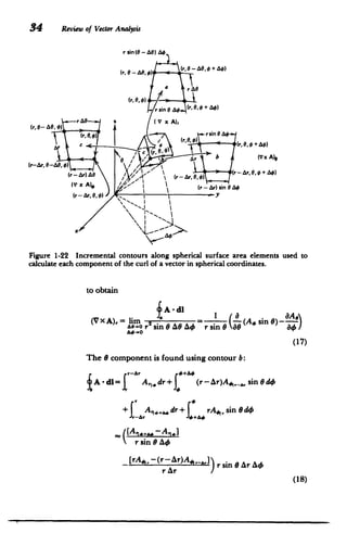
(b) Spherical Coordinates
Similar operations on the three incremental contours for
the spherical element in Figure 1-22 give the curl in spherical
coordinates. We use contour a for the radial component of
the curl:
+ &0 e-A e
A - dl= , A4,r sin 0 dO + rA ,.. dO
+ r sin (0 -A)A 4 .. d+ rA,. dO
.+"4 -As
[A,. sin - A4,.-,. sin (0 - AG))
r sin e AO
[Ae,.. -A _+ r2 sin 0 AO A4 (16)
r sin 0 AO](https://image.slidesharecdn.com/mitres6002s08part1-211102045902/85/Mitres-6-002_s08_part1-61-320.jpg)
![1-5-3 Stokes'
The Curl and Stokes' Theorem 35
as
fA - di
,
(V x A),= lim )(rAo)
Ar-o r sin Ar A4 r sin e a4 4r
A4-0O
(19)
The 4 component of the curl is found using contour c:
8 r--Ar
A-dl= e-, rA1d+ A,[.dr
9-A6
+1 (r-Ar)A _ dG+ J A,,,_,,,dr
([rA,, -(r-Ar)A 1 ,,] [Al, - ArI,,] r Ar AG
rAr r AO
(20)
as
I1 a A,
(V X.A),O = lim =- -(rA,) - (21)
Ar-o r Ar AO r r 81
The curl of a vector in spherical coordinates is thus given
from (17), (19), and (21) as
1
(A. sin 6)
aA
i,
VxA = I
r sin 0 80
+A10 ' Or
nGO4B,
A (rA.4,))i.
r sin 0 a4 ar
+- -(rAe)- a (22)
r ar
Theorem
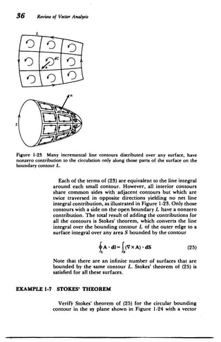
We now piece together many incremental line contours of
the type used in Figures 1-19-1-21 to form a macroscopic
surface S like those shown in Figure 1-23. Then each small
contour generates a contribution to the circulation
dC = (V x A) - dS (23)
so that the total circulation is obtained by the sum of all the
small surface elements
C= f(V x A) - dS (24)](https://image.slidesharecdn.com/mitres6002s08part1-211102045902/85/Mitres-6-002_s08_part1-63-320.jpg)
![38 Review of Vector Analysis
(a) For the circular area in the plane of the contour, we
have that
f (Vx A) - dS = 2 dS. =2rR2
which agrees with the line integral result.
(b) For the hemispherical surface
v/2 2.
(V X A) - dS= = 0 2 - iR2
sin 0dOdO
From Table 1-2 we use the dot product relation
i - i,= cos e
which again gives the circulation as
w/2 2w 2/wco
=
o 0v2 21rR2 C=w22 R 2sin 20 dO d= -21rR
= 11o 2 e-o
(c) Similarly, for th-e cylindrical surface, we only obtain
nonzero contributions to the surface integral at the upper
circular area that is perpendicular to V X A. The integral is
then the same as part (a) as V X A is independent of z.
1-5-4 Some Useful Vector Identities
The curl, divergence, and gradient operations have some
simple but useful properties that are used throughout the
text.
(a) The Curl of the Gradient is Zero [V x (Vf)= 0]
We integrate the normal component of the vector V X (Vf)
over a surface and use Stokes' theorem
JV x (Vf) - dS= Vf - dl= 0 (26)
where the zero result is obtained from Section 1-3-3, that the
line integral of the gradient of a function around a closed
path is zero. Since the equality is true for any surface, the
vector coefficient of dS in (26) must be zero
V X(Vf)=0
The identity is also easily proved by direct computation
using the determinantal relation in Section 1-5-1 defining the](https://image.slidesharecdn.com/mitres6002s08part1-211102045902/85/Mitres-6-002_s08_part1-66-320.jpg)
![Problems 39
curl operation:
i. i, i"
a a
Vx(Vf)det
a
ax ay az
af af af
ax ay az
ix2(L - .) +~, a~f ;a-f)I+i,(AY -~af).0.
ayaz azay azax axaz axay ayax
(28)
Each bracketed term in (28) is zero because the order of
differentiation does not matter.
(b) The Divergence of the Curl of a Vector is Zero
[V -(Vx A)=0]
One might be tempted to apply the divergence theorem to
the surface integral in Stokes' theorem of (25). However, the
divergence theorem requires a closed surface while Stokes'
theorem is true in general for an open surface. Stokes'
theorem for a closed surface requires the contour L to shrink
to zero giving a zero result for the line integral. The diver
gence theorem applied to the closed surface with vector V x A
is then
SV xA -dS =0=V-(VxA)dV=0>V-(VxA)=0
s v (29)
which proves the identity because the volume is arbitrary.
More directly we can perform the required differentiations
V- (VxA)
a, aIA.2 aA,
a faA2 aA. a ,aA aA2
axay az axa ay
/
ay az zax
(a2A. a2A a2A2 a2A 2A, a
x)+(!-x x - -)= 0 (30)
axay ayx ayaz ay azax 0x(z
where again the order of differentiation does not matter.
PROBLEMS
Section 1-1
1. Find the area of a circle in the xy plane centered at the
origin using:
(a) rectangular coordinates x + y2 = a2 (Hint:
2
J- _2 dx = [x a,x
2
+ a2
sin~'(x/a)])](https://image.slidesharecdn.com/mitres6002s08part1-211102045902/85/Mitres-6-002_s08_part1-67-320.jpg)
![40 Review of Vector Atawysis
(b) cylindrical coordinates r= a.
Which coordinate system is easier to use?
2. Find the volume of a sphere of radius R centered at the
origin using:
(a) rectangular coordinates x2+y+z2 = R (Hint:
J 2
(xla)])
1Ia -x dx =[xV/'-x +a'sin-
(b) cylindrical coordinates r2+Z2= R ;
(c) spherical coordinates r = R.
Which coordinate system is easiest?
Section 1-2
3. Given the three vectors
A= 3i.+2i,-i.
B= 3i. -4i, -5i,
C= i. -i,+i,,
find the following:
(a) A-EB,B C,A C
(b) A -B, B -C, A -C
(c) AXB,BXC,AXC
(d) (A x B) - C, A - (B x C) [Are they equal?]
(e) A x (B x C), B(A - C) - C(A - B) [Are they equal?]
(f) What is the angle between A and C and between B and
A xC?
4. Given the sum and difference between two vectors,
A+B= -i.+5i, -4i
A - B = 3i. -i, - 2i,
find the individual vectors A and B.
5. (a) Given two vectors A and B, show that the component
of B parallel to A is
B -A
B1
1= A
A -A
(Hint: Bi = a A. What is a?)
(b) If the vectors are
A = i. - 2i,+i"
B = 3L + 5i, - 5i,
what are the components of B parallel and perpendicular to
A?](https://image.slidesharecdn.com/mitres6002s08part1-211102045902/85/Mitres-6-002_s08_part1-68-320.jpg)
![ProbLems 43
y
A
>x
B
Section 1-3
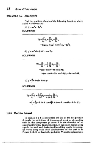
12. Find the gradient of each of the following functions
where a and b are constants:
(a) f=axz+bx-y
(b) f = (a/r) sin 4 + brz cos 34
(c) f = ar cos 0 +(b/r2
) sin 0
13. Evaluate the line integral of the gradient of the function
f=rsin
over each of the contours shown.
Y
2
2a
a
2 -3
-a4
Section 1-4
14. Find the divergence of the following vectors:
(a) A=xi.+ i,+zi. = ri,
(b) A=(xy 2z")i.+i,+ij
(c) A = r cos Oi,+[(z/r) sin 0)]i,
(d) A= r2
sin e cos 4 [i,+i.+i-]
15. Using the divergence theorem prove the following
integral identities:
(a) JVfdV= fdS
M](https://image.slidesharecdn.com/mitres6002s08part1-211102045902/85/Mitres-6-002_s08_part1-71-320.jpg)
![44 Review of Vector Analysis
(Hint: Let A = if, where i is any constant unit vector.)
(b) VxFdV=-fFxdS
(Hint: Let A = iX F.)
(c) Using the results of (a) show that the normal vector
integrated over a surface is zero:
~dS=0
(d) Verify (c) for the case of a sphere of radius R.
(Hint: i, = sin 0 cos i, +sin 0 sin Oi, +cos 8i..
16. Using the divergence theorem prove Green's theorem
f[fVg -gVf] - dS= Jv[fv2g gV2f] dV
(Hint: V . (fVg) = fV2
g + Vf Vg.)
17. (a) Find the area element dS (magnitude and direction)
on each of the four surfaces of the pyramidal figure shown.
(b) Find the flux of the vector
A = ri,.=xi,+yi,+zi,
through the surface of (a).
(c) Verify the divergence theorem by also evaluating the
flux as
b= JV A dV
. 3
a
Section 1-5
18. Find the curl of the following vectors:
(a) A=x2
yi,+y 2
zi,+xyi](https://image.slidesharecdn.com/mitres6002s08part1-211102045902/85/Mitres-6-002_s08_part1-72-320.jpg)
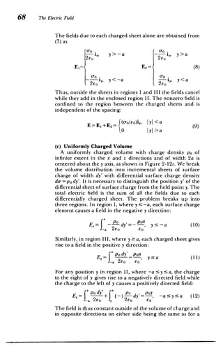
![56 The Electric Field
The parameter Eo is called the permittivity of free space
and has a value
2
eo= (47r X 10-
7
c
10;: 8.8542 X 12 farad/m [A 2
_S
4-- kg' - m 3
] (2)
367r
where c is the speed of light in vacuum (c -3 X 10" m/sec).
This relationship between the speed of light and a physical
constant was an important result of the early electromagnetic
theory in the late nineteenth century, and showed that light is
an electromagnetic wave; see the discussion in Chapter 7.
To obtain a feel of how large the force in (1) is, we compare
it with the gravitational force that is also an inverse square law
with distance. The smallest unit of charge known is that of an
electron with charge e and mass m,
e - 1.60X 10- 19 Coul, m, =9.11 X 10⁻³' kg
Then, the ratio of electric to gravitational force magnitudes
for two electrons is independent of their separation:
F, e'/(47reor2 ) e2 1 42
-= - 2 -4.16 x 10 (3)
F9 GM/r m, 47reoG
where G = 6.67 x 101 [m3
-s~ 2
-kg'] is the gravitational
constant. This ratio is so huge that it exemplifies why elec
trical forces often dominate physical phenomena. The minus
sign is used in (3) because the gravitational force between two
masses is always attractive while for two like charges the
electrical force is repulsive.
2-2-3 The Electric Field
If the charge qi exists alone, it feels no force. If we now
bring charge q2 within the vicinity of qi, then q2 feels a force
that varies in magnitude and direction as it is moved about in
space and is thus a way of mapping out the vector force field
due to qi. A charge other than q2 would feel a different force
from q2 proportional to its own magnitude and sign. It
becomes convenient to work with the quantity of force per
unit charge that is called the electric field, because this quan
tity is independent of the particular value of charge used in
mapping the force field. Considering q2 as the test charge, the
electric field due to qi at the position of q2 is defined as
E2 = lim F= q2 112 volts/m [kg-m-s 3 - A ] (4)
2-o
. q2 4ireor12](https://image.slidesharecdn.com/mitres6002s08part1-211102045902/85/Mitres-6-002_s08_part1-84-320.jpg)
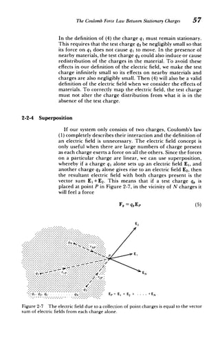
![Charge Distributions 59
2
A
y
q
q [ ri,
a
+ 1-iZ
2___
r
4~E2 [-
E
4e o I
(
==
)2~ r r ( E~) 2
+ 1/2
[2
(
a E E [2
2
+ 2
E
l+E 2 q 2r
r r
+
2] 3/2
Iq ~12
Er q rir - i,
4nreo [r2 +( )2, r2 + ]1)
2/
(a)
y
-q [ rir + i,1
q
ri,
i
2
471 [r +
+3/2
x
(b)
Figure 2-8 Two equal magnitude point charges are a distance a apart along the z
axis. (a) When the charges are of the same polarity, the electric field due to each is
radially directed away. In the z = 0 symmetry plane, the net field component is radial.
(b) When the charges are of opposite polarity, the electric field due to the negative
charge is directed radially inwards. In the z = 0 symmetry plane, the net field is now -z
directed.
The faster rate of decay of a dipole field is because the net
charge is zero so that the fields due to each charge tend to
cancel each other out.
2-3 CHARGE DISTRIBUTIONS
The method of superposition used in Section 2.2.4 will be
used throughout the text in relating fields to their sources.
We first find the field due to a single-point source. Because
the field equations are linear, the net field due to many point](https://image.slidesharecdn.com/mitres6002s08part1-211102045902/85/Mitres-6-002_s08_part1-87-320.jpg)
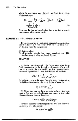
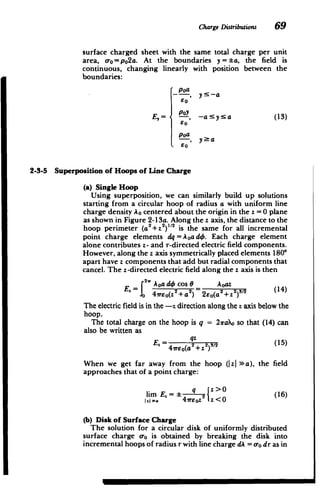
![62 The Electric Field
y y
+
+
P0
a+++
+
+x
++,4
(a) (b) (C)
z
A0
+i (, )2
+
- a
+
:--Q -21/a
3
Ira e
+
x
+
(d) (e)
Figure 2-10 Charge distributions of Example 2-2. (a) Uniformly distributed line
charge on a circular hoop. (b) Uniformly distributed surface charge on a circular disk.
(c) Uniformly distributed volume charge throughout a sphere. (d) Nonuniform line
charge distribution. (e) Smooth radially dependent volume charge distribution
throughout all space, as a simple model of the electron cloud around the positively
charged nucleus of the hydrogen atom.
SOLUTION
2s4= r
q= pdV= f '
'
por sin drdO do = 37TR P0
S= =0 =0
(d) A line charge of infinite extent in the z direction with
charge density distribution
A 0
A =jl(l)
[I +(z/a)
2
1
SOLUTION
q A dl=2 = A 0a tan - Aoira
q j -cj [1+(z/a)2] a](https://image.slidesharecdn.com/mitres6002s08part1-211102045902/85/Mitres-6-002_s08_part1-90-320.jpg)
![ChargeDistributions 63
(e) The electron cloud around the positively charged
nucleus Q in the hydrogen atom is simply modeled as the
spherically symmetric distribution
p(r)=- Q3e 2r/a
Tra
where a is called the Bohr radius.
SOLUTION
The total charge in the cloud is
q= JvpdV
=- f -e -2r/'r 2sin 0 drdO do
,.=, 1=0 f,"- ira
= -- : ~e2T/r2 dr
=- -oa
e -2'' r2
-3 (~ e~' [r2 -- ) 1)] 1_0
= -Q
2-3-2 The Electric Field Due to a Charge Distribution
Each differential charge element dq as a source at point Q
contributes to the electric field at. a point P as
dq
dE= 2 iQp (2)
41rEorQ'
where rQp is the distance between Q and P with iQp the unit
vector directed from Q to P. To find the total electric field, it
is necessary to sum up the contributions from each charge
element. This is equivalent to integrating (2) over the entire
charge distribution, remembering that both the distance rQp
and direction iQp vary for each differential element
throughout the distribution
dq
E = q Q2 (3)
111, 417rEor Qp
where (3) is a line integral for line charges (dq = A dl), a
surface integral for surface charges (dq = o-dS), a volume](https://image.slidesharecdn.com/mitres6002s08part1-211102045902/85/Mitres-6-002_s08_part1-91-320.jpg)
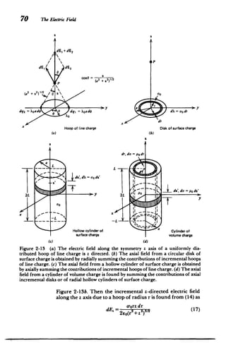
![ChargeDistributions 71
where we replace a with r, the radius of the incremental
hoop. The total electric field is then
a rdr
O-oz 2 2 1/2
2EE Jo (r +z
)
oJoz
2eo(r2
+Z
2
V1 2
o
_ ( _ z z
2E (
2eo '(a 2 +z2) )u
1/2 I
+z Izi/
_roz
(18)
z >0
2eo 2eo(a 2+z2
) 1z<0 (1
where care was taken at the lower limit (r = 0), as the magni
tude of the square root must always be used.
As the radius of the disk gets very large, this result
approaches that of the uniform field due to an infinite sheet
of surface charge:
lim E = z>0(19)
a-00 2co 1z <0
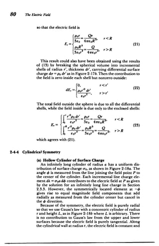
(c) Hollow Cylinder of Surface Charge
A hollow cylinder of length 2L and radius a has its axis
along the z direction and is centered about the z =0 plane as
in Figure 2-13c. Its outer surface at r=a has a uniform
distribution of surface charge ao. It is necessary to distinguish
between the coordinate of the field point z and the source
point at z'(-L sz':5L). The hollow cylinder is broken up
into incremental hoops of line charge dA = ordz'. Then, the
axial distance from the field point at z to any incremental
hoop of line charge is (z -z'). The contribution to the axial
electric field at z due to the incremental hoop at z' is found
from (14) as
dE = aoa(z - z') dz' (20)
- z') 2
]31 2
2Eo[a
2 +(z
which when integrated over the length of the cylinder yields
ooa [L (z - z') dz'
Ez 2eO .L [a2
+(z - z')
2
3 1 2
o-oa *1
2eo [a2 +(z -z') 2 'L
[a L) 2
[a2+( +L)211/2) (21)
2
+(z 1/2](https://image.slidesharecdn.com/mitres6002s08part1-211102045902/85/Mitres-6-002_s08_part1-99-320.jpg)
![72 The Electric Field
(d) Cylinder of Volume Charge
If this same cylinder is uniformly charged throughout the
volume with charge density po, we break the volume into
differential-size hollow cylinders of thickness dr with incre
mental surface charge do-=po dr as in Figure 2-13d. Then, the
z-directed electric field along the z axis is obtained by integra
tion of (21) replacing a by r:
E. =-LO- f r( 2 -2122 2 12 dr
2E 0 Jo [r +(z -L) [r +(z+L) I
/
[r2+(Z+L)2]1/21 = {[r2+(Z -L)1/2 2
2eo
=-- -{[a2+(z -L)2 ]1-Iz -LI -[a 2
+(z +L) 2
1/
2
2Eo
+Iz+LL} (22)
where at the lower r=0 limit we always take the positive
square root.
This problem could have equally well been solved by
breaking the volume charge distribution into many differen
tial-sized surface charged disks at position z'(-L z':L),
thickness dz', and effective surface charge density do =po dz'.
The field is then obtained by integrating (18).
2-4 GAUSS'S LAW
We could continue to build up solutions for given charge
distributions using the coulomb superposition integral of
Section 2.3.2. However, for geometries with spatial sym
metry, there is often a simpler way using some vector prop
erties of the inverse square law dependence of the electric
field.
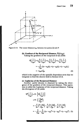
2-4-1 Properties of the Vector Distance Between Two Points, rop
(a) rop
In Cartesian coordinates the vector distance rQp between a
source point at Q and a field point at P directed from Q to P
as illustrated in Figure 2-14 is
r2p= (x -XQ)i + (y - yQ)i, +(z - Z()I (1)
with magnitude
rQp=[(x xQ)2+(y yQ)2 +(z -ZQ)2 ]1 (2)
The unit vector in the direction of rQp is
IQP = rQP (3)
rQP](https://image.slidesharecdn.com/mitres6002s08part1-211102045902/85/Mitres-6-002_s08_part1-100-320.jpg)
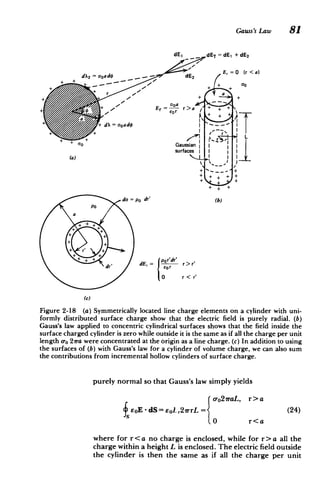
![Gauss's Law 77
dE
dq2=aoR 2sin 0dd
A.. - d
Er Q
41ror2
Total
surface
S- charge
2
. Q=47rR o0
rgp +
0 R
+
r
+
dqi =ooR
2
sinOdOdo
/
+
+
Q enclosed
Q =4aR2)0
Gaussian
No Iag
No charge (spheres
enclosed s
(a) (b)
Figure 2-16 A sphere of radius R with uniformly distributed surface charge o-,. (a)
Symmetrically located charge elements show that the electric field is purely radial. (b)
Gauss's law, applied to concentric spherical surfaces inside (r< R) and outside (r > R)
the charged sphere, easily shows that the electric field within the sphere is zero and
outside is the same as if all the charge Q = 47rR Oro were concentrated as a point charge
at the origin.
encloses all the charge Q = o-o4-irR
2
}ro47rR 2
= Q, r>R
EOE - dS = EOE,47r2 = (12)
0, r<R
so that the electric field is
o-oR2
2= ] 2, r>R
E= eor 47eor (13)
0, r<R
The integration in (12) amounts to just a multiplication of
eoE, and the surface area of the Gaussian sphere because on
the sphere the electric field is constant and in the same direc
tion as the normal ir. The electric field outside the sphere is
the same as if all the surface charge were concentrated as a
point charge at the origin.
The zero field solution for r <R is what really proved
Coulomb's law. After all, Coulomb's small spheres were not
really point charges and his measurements did have small
sources of errors. Perhaps the electric force only varied
inversely with distance by some power close to two, r-2
where 8 is very small. However, only the inverse square law](https://image.slidesharecdn.com/mitres6002s08part1-211102045902/85/Mitres-6-002_s08_part1-105-320.jpg)
![78 The Electric Field
gives a zero electric field within a uniformly surface charged
sphere. This zero field result-is true for any closed conducting
body of arbitrary shape charged on its surface with no
enclosed charge. Extremely precise measurements were made
inside such conducting surface charged bodies and the
electric field was always found to be zero. Such a closed
conducting body is used for shielding so that a zero field
environment can be isolated and is often called a Faraday
cage, after Faraday's measurements of actually climbing into
a closed hollow conducting body charged on its surface to
verify the zero field results.
To appreciate the ease of solution using Gauss's law, let us
redo the problem using the superposition integral of Section
2.3.2. From Figure 2-16a the incremental radial component
of electric field due to a differential charge element is
c-oR2
sin eded
dE,- 42sn cos a (14)
From the law of cosines the angles and distances are related as
2 2 2
rQp r +R -2rR cos 0
2 2 2 (5
R =r +rQP-2rrQpcosa
so that a is related to 0 as
r-R cos 0
[r +R -2rR cos9]
2 (16)
Then the superposition integral of Section 2.3.2 requires us
to integrate (14) as
r. f 2 o-oR2
sin 8(r-R cos 0) d0
d4
E 6=0 = 41reo[r+R-2rR cos 01 ('
After performing the easy integration over 4 that yields the
factor of 21r, we introduce the change of variable:
u =r2 +R 2-2rR cos 6
du = 2rR sin dG (18)
which allows us to rewrite the electric field integral as
(r+R)2
2 2 dU
Er oR[u+r -R]d
= 2 3/2
2
-R2 ) (r+R)2
OR U1/2 _(r
4eUr2
112 I I(r-R)2
o-oR (r+R)-|r-RI -(r 2
-R) (rR_ 12)
R -RI)
(19)](https://image.slidesharecdn.com/mitres6002s08part1-211102045902/85/Mitres-6-002_s08_part1-106-320.jpg)
![86 The Electric Field
curl of the electric field:
E -dl= (V XE) -dS (4)
From Section 1.3.3, we remember that the gradient of a scalar
function also has the property that its line integral around a
closed path is zero. This means that the electric field can be
determined from the gradient of a scalar function V called
the potential having units of volts [kg-m 2-s-3
-A-]:
E = -V V (5)
The minus sign is introduced by convention so that the elec
tric field points in the direction of decreasing potential. From
the properties of the gradient discussed in Section 1.3.1 we
see that the electric field is always perpendicular to surfaces of
constant potential.
By applying the right-hand side of (4) to an area of
differential size or by simply taking the curl of (5) and using
the vector identity of Section 1.5.4a that the curl of the
gradient is zero, we reach the conclusion that the electric field
has zero curl:
VxE=O (6)
2-5-3 The Potential and the Electric Field
The potential difference between the two points at ra and rb
is the work per unit charge necessary to move from ra to rb:
w
V(rb)- V(ra)=-
Jrb fS 7
=f E - dl= + E - dl (7)
Note that (3), (6), and (7) are the fields version of Kirchoff's
circuit voltage law that the algebraic sum of voltage drops
around a closed loop is zero.
The advantage to introducing the potential is that it is a
scalar from which the electric field can be easily calculated.
The electric field must be specified by its three components,
while if the single potential function V is known, taking its
negative gradient immediately yields the three field
components. This is often a simpler task than solving for each
field component separately. Note in (5) that adding a constant
to the potential does not change the electric field, so the
potential is only uniquely defined to within a constant. It is
necessary to specify a reference zero potential that is often](https://image.slidesharecdn.com/mitres6002s08part1-211102045902/85/Mitres-6-002_s08_part1-114-320.jpg)
![The Electric Potential 89
The field components are obtained from (13) by taking the
negative gradient of the potential:
aV Ao 1 1
E. = --- = -- 2 (Z + L )21/2
z 4E [r2+(Z - L )21/2
aV
Br 4wreo[r
Aor +(z -L)2 ]sz- I +[r
+(zL)2
Er=- = 2+ Z )11[ +Z 2l2
ar 47reo [r +(-L) 2
"[-L+[r (-)]]
[r2+(z+L)2 2[z+L+[r +(z+L)2]/2
SAo( z-L z+L
47reor [r2
+(z -L) 2
]1 2
[r2
+(+L)
2
]1 2
) (14)
As L becomes large, the field and potential approaches that
of an infinitely long line charge:
E= 0
=A
o
E, =k (15)
lim 27reor
-
V= (In r -ln 2L)
21rso
The potential has a constant term that becomes infinite
when L is infinite. This is because the zero potential reference
of (10) is at infinity, but when the line charge is infinitely long
the charge at infinity is nonzero. However, this infinite
constant is of no concern because it offers no contribution to
the electric field.
Far from the line charge the potential of (13) approaches
that of a point charge 2AoL:
lim V=Ao(2L) (16)
2 2
>L2
r +z 47rEor
Other interesting limits of (14) are
E. =0
lim AL
r
E 27reor(r2+L2)2
AoL z>L
A 2reo(z2
-L 2
)' z<-L
~E =A-( 1 ___
lim 47rEo L |z+L| z -LIL|
r= rE(L2
Z2
), -LzsL
Er=0 (17)
M](https://image.slidesharecdn.com/mitres6002s08part1-211102045902/85/Mitres-6-002_s08_part1-117-320.jpg)
![94 The Electric Field
line charge from Section 2.3.3 allows us to obtain the poten
tial by direct integration:
av A A r
Er= - >V=- In- (1)
ar 21Teor 27reo ro
where ro is the arbitrary reference position of zero potential.
If we have two line charges of opposite polarity A a
distance 2a apart, we choose our origin halfway between, as
in Figure 2-24a, so that the potential due to both charges is
just the superposition of potentials of (1):
A y2+(x+ a)212 (2)
V= - 2ireoIn y 2
+(xa)(2)
where the reference potential point ro cancels out and we use
Cartesian coordinates. Equipotential lines are then
y +(x+a) -4, V/=K (3)
0
y +(xa)2e
where K1 is a constant on an equipotential line. This relation is
rewritten by completing the squares as
a(+K) 2 2= 4Ka2(4)
Ki1(I-K')2
which we recognize as circles of radius r=2a/ Ki I-Kd
with centers at y=0,x=a(1+K1)/(Ki-1), as drawn by
dashed lines in Figure 2-24b. The value of K1 = 1 is a circle of
infinite radius with center at x = 0 and thus represents the
x=0 plane. For values of K 1 in the interval OsK1
1 1 the
equipotential circles are in the left half-plane, while for 1:5
K1 ! oo the circles are in the right half-plane.
The electric field is found from (2) as
A (-4axyi+2a(y2 +a2_ 2
E=-VV= 221 (5)
27rEn [y2+(x+a)
2
][Y2
+(x-a)2
One way to plot the electric field distribution graphically is
by drawing lines that are everywhere tangent to the electric
field, called field lines or lines of force. These lines are
everywhere perpendicular to the equipotential surfaces and
tell us the direction of the electric field. The magnitude is
proportional to the density of lines. For a single line charge,
the field lines emanate radially. The situation is more compli
cated for the two line charges of opposite polarity in Figure
2-24 with the field lines always starting on the positive charge
and terminating on the negative charge.](https://image.slidesharecdn.com/mitres6002s08part1-211102045902/85/Mitres-6-002_s08_part1-122-320.jpg)
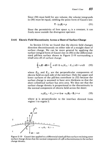
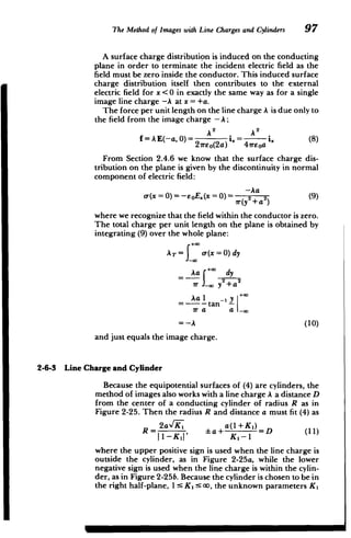
![The Method of Images with Line Chargesand Cylinders 95
y
S y
2
+ x+ a)
2
2 2
4re
o 1y +(xaf
1
2 2 2 2
[y + (x + a) ] 112 [y +{ x-a
2
1V
x
-a a
(a)
y
Field lines Equipotential lines - - -
2
)2 92 al1 +K,) 2 4a2 K,
x2 + (y- a cotK2
x ~ sin
a2
K2 K, -1 1-K,)
-N
iIi
1E /a
x
N
- /1
N
N
N
N
N
N
aI
7 <K,1
O~K1 1
Figure 2-24 (a) Two parallel line charges of opposite polarity a distance 2a apart. (b)
The equipotential (dashed) and field (solid) lines form a set of orthogonal circles.](https://image.slidesharecdn.com/mitres6002s08part1-211102045902/85/Mitres-6-002_s08_part1-123-320.jpg)
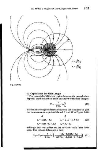
![The Method of Images with Line Chargesand Cylinders 99
The force per unit length on the cylinder is then just due to
the force on the image charge:
A2
A 2
D
(14)
2feo(D-b) 27reo(D
2
-R2
)
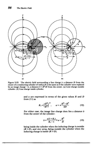
2-6-4 Two Wire Line
(a) Image Charges
We can continue to use the method of images for the case
of two parallel equipotential cylinders of differing radii R,
and R 2 having their centers a distance D apart as in Figure
2-26. We place a line charge A a distance b, from the center of
cylinder 1 and a line charge -A a distance b2 from the center
of cylinder 2, both line charges along the line joining the
centers of the cylinders. We simultaneously treat the cases
where the cylinders are adjacent, as in Figure 2-26a, or where
the smaller cylinder is inside the larger one, as in Figure
2-26b.
The position of the image charges can be found using (13)
realizing that the distance from each image charge to the
center of the opposite cylinder is D - b so that
R2
bi= ,2 b2= i (15)
D-F b2 D-b
where the upper signs are used when the cylinders are
adjacent and lower signs are used when the smaller cylinder is
inside the larger one. We separate the two coupled equations
in (15) into two quadratic equations in b, and b 2:
bi - b,+R =0
b2- D b2+R2 0
with resulting solutions
2 2 2 2 2 112
[D -R +R 2 ] D -R +R2 2
b2= 2D 2D )-)R2
S2 2 2(17)
b=[D +R 1 -R 2 ] D +R -R(17)
2D L 2D / i
We were careful to pick the roots that lay outside the region
between cylinders. If the equal magnitude but opposite
polarity image line charges are located at these positions, the
cylindrical surfaces are at a constant potential.](https://image.slidesharecdn.com/mitres6002s08part1-211102045902/85/Mitres-6-002_s08_part1-127-320.jpg)
![100 The Electric Field
b,= b2 A2 D-b
Figure 2-26 The solution for the electric field between two parallel conducting
cylinders is found by replacing the cylinders by their image charges. The surface
charge density is largest where the cylinder surfaces are closest together. This is called
the proximity effect. (a) Adjacent cylinders. (b) Smaller cylinder inside the larger one.
(b) Force of Attraction
The attractive force per unit length on cylinder 1 is the
force on the image charge A due to the field from the
opposite image charge -A:
A 2
27reo[ (D - bi)- b
2]
A 2
D2
-R2+R 2 1 2
417Eo 2D R
A
2
2
2 2 2
- ~ 2]1/ (18)
D -R2+Rl 2 v
ITEoR 2D R](https://image.slidesharecdn.com/mitres6002s08part1-211102045902/85/Mitres-6-002_s08_part1-128-320.jpg)
![D
2
2
(
102 The Electric Field
This expression can be greatly reduced using the relations
DFb 2 = , D-b =:- (22)
bI 1
b
2
to
A bib2
Vi- V2=- In i
21reo R1R 2
2 2 2
A I [D -R 1 -R 2 1
2 reo
1 2R1R2
[(D2
-R 2
2 2 1/2
+ D R )-1]} (23)
R2RIR2
The potential difference V1 - V2 is linearly related to the
line charge A through a factor that only depends on the
geometry of the conductors. This factor is defined as the
capacitance per unit length and is the ratio of charge per unit
length to potential difference:
'r-
2
t 2reo1/2 C A 2
2
2 2
I - V2n E [D -R1-R + D-R, -Ri 1*
2R1R 2 2R1 R 2
21reo
cosh~ 1
2
2RIR2
where we use the identity*
_
1)
1 2
In [y+(y 2
]= cosh~1 y (25)
We can examine this result in various simple limits.
Consider first the case for adjacent cylinders (D > R1 + R2 ).
1. If the distance D is much larger than the radii,
lim C In 2reo 2ro (26)
Dm(RA+RO In [D2/(RIR 2)] cosh-' [D2/(2RIR2)]
2. The capacitance between a cylinder and an infinite plane
can be obtained by letting one cylinder have infinite
radius but keeping finite the closest distance s =
*y =cosh x= ex + e
2
(e')2
-2ye"+ 1= 0
e' = y /
2
n(y2) 1
x =cosh-'y =In [y: (y 2- 1)"12]](https://image.slidesharecdn.com/mitres6002s08part1-211102045902/85/Mitres-6-002_s08_part1-130-320.jpg)
![The Method of Images with Point Charges and Spheres 103
D-RI-R 2 between cylinders. If we let R1 become
infinite, the capacitance becomes
lim C = 2 s+R 2 1/2
D-R,-R 2 = (finite) In sR 2 + R 2
27TEo (27)
coshW ( +R
)
2
3. If the cylinders are identical so that R 1 =R2 =R, the
capacitance per unit length reduces to
lim C= 2 1 = (28)
R,=R 2 =R D sDh _ D
In T+1
- 1- cosh' D 28
2R L2R) 2R
4. When the cylinders are concentric so that D=0, the
capacitance per unit length is
21m)o 27rE o
lim C= = 2 2 (29)
D O In (R]/R2) cosh- [(RI + R2)/(2R, R2)]
2-7 THE METHOD OF IMAGES WITH POINT CHARGES AND
SPHERES
2-7-1 Point Charge and a Grounded Sphere
A point charge q is a distance D from the center of the
conducting sphere of radius R at zero potential as shown in
Figure 2-27a. We try to use the method of images by placing a
single image charge q' a distance b from the sphere center
along the line joining the center to the point charge q.
We need to find values of q' and b that satisfy the zero
potential boundary condition at r = R. The potential at any
point P outside the sphere is
(
1 !+
4,reo s s
where the distance from P to the point charges are obtained
from the law of cosines:
s =[r2+ 2 -2rD cos 6]0 2
(
s'= [b2
+r2
-2rb cos 011/2](https://image.slidesharecdn.com/mitres6002s08part1-211102045902/85/Mitres-6-002_s08_part1-131-320.jpg)
![(4 The Electric Field
I
Conducting sphere
at zero potential
s s, r
qR
q
q D x
Inducing charge b =
0utside sphere D
C -D
(a)
Inducing charge R
inside sphere
qR
b R
'2
D
Figure 2-27 (a) The field due to a point charge q, a distance D outside a conducting
sphere of radius R, can be found by placing a single image charge -qRID at a distance
b = R'ID from the center of the sphere. (b) The same relations hold true if the charge
q is inside the sphere but now the image charge is outside the sphere, since D < R.
At r = R, the potential in (1) must be zero so that q and q'
must be of opposite polarity:
+S) = > 9) = (3)
where we square the equalities in (3) to remove the square
roots when substituting (2),
q 2
[b2
+ R2-2Rb cos 6] = q'2
[R 2+D2
-2RD cos 0] (4)](https://image.slidesharecdn.com/mitres6002s08part1-211102045902/85/Mitres-6-002_s08_part1-132-320.jpg)
![The Method of Images with PointCharges andSpheres 105
Since (4) must be true for all values of 0, we obtain the
following two equalities:
q2
(b 2
+R 2
) q 2
(R 2
+D 2
)
qub=q'2D(5
Eliminating q and q' yields a quadratic equation in b:
b2-bD 1+ R +R 2
=0 (6)
with solution
Db 2
] + -2
b=- - [1+-1
-
2 L R2/2
-{1+( )I1(R (7)
We take the lower negative root so that the image charge is
inside the sphere with value obtained from using (7) in (5):
R2
R
b= , q= -q (8)
DD
remembering from (3) that q and q' have opposite sign. We
ignore the b = D solution with q'= -q since the image charge
must always be outside the region of interest. If we allowed
this solution, the net charge at the position of the inducing
charge is zero, contrary to our statement that the net charge
is q.
The image charge distance b obeys a similar relation as was
found for line charges and cylinders in Section 2.6.3. Now,
however, the image charge magnitude does not equal the
magnitude of the inducing charge because not all the lines of
force terminate on the sphere. Some of the field lines
emanating from q go around the sphere and terminate at
infinity.
The force on the grounded sphere is then just the force on
the image charge -q' due to the field from q:
qq _ q2
R _ q2
RD
2 2
)2
4vreo(D - b)2
- 41reoD(D-b) 4irEo(D2
-R (9)](https://image.slidesharecdn.com/mitres6002s08part1-211102045902/85/Mitres-6-002_s08_part1-133-320.jpg)
![106 The Electric Field
The electric field outside the sphere is found from (1) using
(2) as
E= -V V= (![(r-D cos 0)i,+Dsin i,]
4vreos
+- [(r- b cos 6)i, +b sin ie]) (10)
On the sphere where s'= (RID)s, the surface charge dis
tribution is found from the discontinuity in normal electric
field as given in Section 2.4.6:
q(D2 - R2)
o-(r = R)= eoE,(r = R)= 41rR[R2 +D 2
-2RD cos 013/2
(11)
The total charge on the sphere
qT= o-(r=R)2rR2
sin 0dG
= -R (D2- R 2
) 22 sin 0d 2 (12)
2 0 [R +D -2RD cos
can be evaluated by introducing the change of variable
u=R2+D -2RD cos 0, du = 2RD sin 0 d6 (13)
so that (12) integrates to
q(D2
-R 2
) (D+R9 du
2
4D (D-R) U
2
q(D 2
-R
2
) 2 (D+R) qR
4D u / 1(D-R)
2
D (14)
which just equals the image charge q'.
If the point charge q is inside the grounded sphere, the
image charge and its position are still given by (8), as illus
trated in Figure 2-27b. Since D < R, the image charge is now
outside the sphere.
2-7-2 Point Charge Near a Grounded Plane
If the point charge is a distance a from a grounded plane,
as in Figure 2-28a, we consider the plane to be a sphere of
infinite radius R so that D = R + a. In the limit as R becomes
infinite, (8) becomes
R
lim q'= -q, b R =R-a (15)
R00 (1+a/R)
D=R+a](https://image.slidesharecdn.com/mitres6002s08part1-211102045902/85/Mitres-6-002_s08_part1-134-320.jpg)
![The Method of Images with PointChargesand Spheres 107
. Eo.i.
q
image charge
image charge
(a) (b)
Figure 2-28 (a) A point charge q near a conducting plane has its image charge --q
symmetrically located behind the plane. (b) An applied uniform electric field causes a
uniform surface charge distribution on the conducting plane. Any injected charge
must overcome the restoring force due to its image in order to leave the electrode.
so that the image charge is of equal magnitude but opposite
polarity and symmetrically located on the opposite side of the
plane.
The potential at any point (x, y, z) outside the conductor is
given in Cartesian coordinates as
I
V=q I
47rEo ([(x + a)2 +y2 + Z2112 [(x -- a)2+y2 + z2112) (6
with associated electric field
E=-VV= q (x +a)i.+ yi, +zi, (x-a)i,+yi,+zi*.,
47reo [(x + a )2+y2 + Z2]s12- _( +zZ 29
-a)2 +y2
(17)
Note that as required the field is purely normal to the
grounded plane
E,(x = 0) =0, E,(x = 0) = 0 (18)
The surface charge density on the conductor is given by the
discontinuity of normal E:
or(x = 0)=-eoE.(x= 0)
_q 2a
41r [y 2+ z2+a2]3/2
(19)
27rr4
qa 23/2; r2=2+ Z2
where the minus sign arises because the surface normal
points in the negative x direction.](https://image.slidesharecdn.com/mitres6002s08part1-211102045902/85/Mitres-6-002_s08_part1-135-320.jpg)
![Problems 115
when:
(a) the charges have the same polarity, q, = q2 q3= q4= q;
(b) the charges alternate in polarity, qI = q3 q, q2 = q4
-q;
(c) the charges are q, =q2q, q3=q4-q.
Section 2.3
12. Find the total charge in each of the following dis
tributions where a is a constant parameter:
(a) An infinitely long line charge with density
,k(z) Ao e-IZI /a
(b) A spherically symmetric volume charge distributed
over all space
p(r)= P 4
[1 +r/a]
4
(Hint: Let u = 1+ r/a.)
(c) An infinite sheet of surface charge with density
o~oe-I x1 /a
[I+(y/b) 2
]
13. A point charge q with mass M in a gravity field g is
released from rest a distance xO above a sheet of surface
charge with uniform density 0-0.
* q
(a) What is the position of the charge as a function of time?
(b) For what value of o-o will the charge remain stationary?
(c) If o-o is less than the value of (b), at what time and with
what velocity will the charge reach the sheet?
14. A point charge q at z = 0 is a distance D away from an
infinitely long line charge with uniform density Ao.
+ (a) What is the force on the point charge q?
+ (b) What is the force on the line charge?
+ (c) Repeat (a) and (b) if the line charge has a distribution
+ Ao1I
+
+0q
_A(z)=
~ Y a
D :](https://image.slidesharecdn.com/mitres6002s08part1-211102045902/85/Mitres-6-002_s08_part1-143-320.jpg)
![Problems 119
+ + + +
+
+ + + + + +a /
+ + + +
+
+
+
+
+z
x
of the circle. Hint:
xdx -1
J [x+2 23/2 2 +a21/2
dx _ _
=2[X2 21/12
2
J [x2
+a2
] a [x +a ]
i,= cos 4 i. + sin 4 i,
Section 2.4
22. Find the total charge enclosed within each of the follow
ing volumes for the given electric fields:
(a) E = Ar2
i, for a sphere of radius R;
(b) E= A r2
i, for a cylinder of radius a and length L;
(c) E = A (xi, +yi,) for a cube with sides of length a having
a corner at the origin.
23. Find the electric field everywhere for the following
planar volume charge distributions:
(a) p(x)=poe*, -00: x5 00
P(X)
-b s x 5--a
-O -P (b) p () -po,
- po
IP0, a &x - b
b
p(x)
PO
-d pox
d (c) p(x)-, -d x d
d d
~~PO
M M](https://image.slidesharecdn.com/mitres6002s08part1-211102045902/85/Mitres-6-002_s08_part1-147-320.jpg)
![120 The Eledric Field
pIx)
Po
x (d) (x) po(1+xld), -d sx O0
-d d Ipo(I - xd), 0:5x:5
24. Find the electric field everywhere for the following
spherically symmetric volume charge distributions:
(a) p(r)=poe~'", Osr5oo
Hint: J r2
e"a dr = -a e-""[r
2
+2a 2
(r/a +1)].)
(b p(r =pi, Osr<Rl
P2, R 1<r<R
2
(c) p(r)=por/R, O<r<R
25. Find the electric field everywhere for the following
cylindrically symmetric volume charge distributions:
(a) p(r)=poer"/, O<r<oo
[Hint: J re radr=-a 2-ra(r/a+ 1).
O<r<a
(b) p(r)= pi,
IP2, a<r<b
(c) p(r)=por/a, O<r<a
y
... ...
.. '..p
rir =Xi, +yiY
S r b r'i,.={x-di,+yiy
X
..................
if . .....
*
... *.
26. An infinitely long cylinder of radius R with uniform
volume charge density po has an off-axis hole of radius b with
center a distance d away from the center of the cylinder.](https://image.slidesharecdn.com/mitres6002s08part1-211102045902/85/Mitres-6-002_s08_part1-148-320.jpg)
![Probems 123
(b) What is the potential along the z axis due to this incre
mental charged hoop? Eliminate the dependence on 8 and
express all variables in terms of z', the height of the differen
tial hoop of line charge.
(c) What is the potential at any position along the z axis
due to the entire hemisphere of surface charge? Hint:
dz' 2,a+bz'
f [a+bz'] 2
s= b
(d) What is the electric field along the z axis?
(e) If the hemisphere is uniformly charged throughout its
volume with total charge Q, find the potential and electric
field at all points along the z axis. (Hint: JrvIz"+r dr=
} (z2+r 2
)3
/2.)
33. Two point charges qi and q2 lie along the z axis a distance
a apart.
((. 0 t)
ri
qE
ay
q2
x
(a) Find the potential at the coordinate (r, 0,th
(Hint: r2 = r + (a/2)2
Har cos 0.)
(b) What is the electric field?
(c) An electric dipole is formed if q2 =-ql. Find an
approximate expression for the potential and electric field for
points far from the dipole, r a.
(d) What is the equation of the. field lines in this far field
limit that is everywhere tangent to the electric field
dr Er
r dG Ea
Find the equation of the field line that passes through the
point (r = ro, 0 = 7r/2). (Hint: I cot 0 dO = In sin 0.)
34. (a) Find the potentials V1, V2, and V3 at the location of
each of the three-point charges shown.](https://image.slidesharecdn.com/mitres6002s08part1-211102045902/85/Mitres-6-002_s08_part1-151-320.jpg)
![The Electric Field
(a) Find the electric field everywhere in the yz plane.
(Hint: Break the sheet into differential line charge elements
dA = aody'.)
(b) An infinitely long conducting cylinder of radius a sur
rounds the charged sheet that has one side along the axis of
the cylinder. Find the image charge and its location due to an
incremental line charge element uo dy' at distance y'.
(c) What is the force per unit length on the cylinder?
Hint:
In (I -cy') dy'= - ccy [In (I -cy')- 1]
37. A line charge A is located at coordinate (a, b) near a
right-angled conducting corner.
y
7Y
(a
S~b) * a,
b)
x
(a) (d)
(a) Verify that the use of the three image line charges
shown satisfy all boundary conditions.
(b) What is the force per unit length on A?
(c) What charge per unit length is induced on the surfaces
x=0 and y =0?
(d) Now consider the inverse case when three line charges
of alternating polarity tA are outside a conducting corner.
What is the force on the conductor?
(e) Repeat (a)-(d) with point charges.
Section 2.7
38. A positive point charge q within a uniform electric field
Eoi2 is a distance x from a grounded conducting plane.
(a) At what value of x is the force on the charge equal to
zero?
(b) If the charge is initially at a position equal to half the
value found in (a), what minimum initial velocity is necessary
for the charge to continue on to x = +o? (Hint: E.=
-dVdx.)](https://image.slidesharecdn.com/mitres6002s08part1-211102045902/85/Mitres-6-002_s08_part1-154-320.jpg)
![128 The Electric Field
I;
4QP
R R
L
(a) Consider the incremental charge element Ao dz' a dis
tance rQp from the sphere center. What is its image charge
and where is it located?
(b) What is the total charge induced on the sphere? Hint:
=In (z'+vR7+z'Y)
42. A conducting hemispherical projection of radius R is
placed upon a ground plane of infinite extent. A point
charge q is placed a distance d (d > R) above the center of the
hemisphere.
i
qI
d
if R
-*7Y
(a) What is the force on q? (Hint: Try placing three
image charges along the z axis to make the plane and hemi
sphere have zero potential.)
(b) What is the total charge induced on the hemisphere at
r = R and on the ground plane IyI > R? Hint:
rdr -1
2
[r2
+d2
] 1
/
2
vr+d](https://image.slidesharecdn.com/mitres6002s08part1-211102045902/85/Mitres-6-002_s08_part1-156-320.jpg)
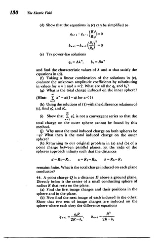
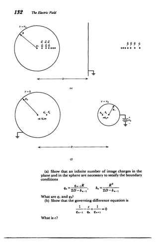
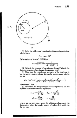
![ProbLems 131
SQ
D
®R
(c) Eliminating the b., show that the governing difference
equation is
1 2 1
--- -+-= 0
q.+, q. q.-I
Guess solutions of the form
P = l/q = AA'
and find the allowed values of A that satisfy the difference
equation. (Hint: For double roots of A the total solutidn is of
the form P. = (A1 + A 2n)A".)
(d) Find all the image charges and their positions in the
sphere and in the plane.
(e). Write the total charge induced on the sphere in the
form
* A
qT= Y 2
n=1[1-an ]
What are A and a?
(f) We wish to generalize this problem to that of a sphere
resting on the ground plane with an applied field E = -Eoi. at
infinity. What must the ratio QID 2
be, such that as Q and D
become infinite the field far from the sphere in the 6 = vr/2
plane is -Eoi.?
(g) In this limit what is the total charge induced on the
sphere? (Hint: Y - Vr/6.)
45. A conducting sphere of radius R at potential Vo has its
center a distance D from an infinite grounded plane.](https://image.slidesharecdn.com/mitres6002s08part1-211102045902/85/Mitres-6-002_s08_part1-159-320.jpg)
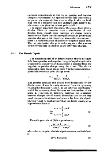
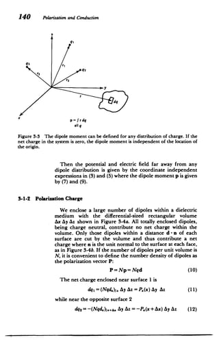
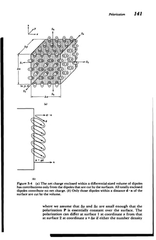
![Polarization 139
Because the separation of atomic charges is on the order of
1 A(10 10 m) with a charge magnitude equal to an integer
multiple of the electron charge (q = 1.6 X 10⁻¹⁹ coul), it is
convenient to express dipole moments in units of debyes
defined as I debye = 3.33 X1030 coul-m so that dipole
moments are of order p = 1.6 x 10⁻²⁹ coul-m - 4.8 debyes.
The electric field for the point dipole is then
P 3
(p-i,),- p ()
E= -V V= 3
[2 cos Oi,+sin Gbi]= 3 (5)
47rEor 47rEor
the last expressions in (3) and (5) being coordinate indepen
dent. The potential and electric field drop off as a single
higher power in r over that of a point charge because the net
charge of the dipole is zero. As one gets far away from the
dipole, the fields due to each charge tend to cancel. The point
dipole equipotential and field lines are sketched in Figure
3-2b. The lines tangent to the electric field are
dr =-=2cot->r=rosin2
(6)
rd6 EO
where ro is the position of the field line when 6 = 7r/2. All field
lines start on the positive charge and terminate on the nega
tive charge.
If there is more than one pair of charges, the definition of
dipole moment in (4) is generalized to a sum over all charges,
p= Y qiri (7)
all charges
where ri is the vector distance from an origin to the charge qj
as in Figure 3-3. When the net charge in the system is zero
(_ qj =0), the dipole moment is independent of the choice of
origins for if we replace ri in (7) by ri +ro, where ro is the
constant vector distance between two origins:
p= qi(ri + ro)
0
=_ q qi
gri +ro
=Y_
qiri (8)
The result is unchanged from (7) as the constant ro could be
taken outside the summation.
If we have a continuous distribution of charge (7) is further
generalized to
(9)
P all qr dq](https://image.slidesharecdn.com/mitres6002s08part1-211102045902/85/Mitres-6-002_s08_part1-167-320.jpg)
![Polarization 145
(b) The Local Electric Field
If this dipole were isolated, the local electric field would
equal the applied macroscopic field. However, a large
number density N of neighboring dipoles also contributes to
the polarizing electric field. The electric field changes dras
tically from point to point within a small volume containing
many dipoles, being equal to the superposition of fields due
to each dipole given by (5). The macroscopic field is then the
average field over this small volume.
We calculate this average field by first finding the average
field due to a single point charge Q a distance a along the z
axis from the center of a spherical volume with radius R
much larger than the radius of the electron cloud (R >> Ro) as
in Figure 3-5b. The average field due to this charge over the
spherical volume is
f Q(ri,-ai )r'sin Odrd d,
<( 3
E >* 2 2 -2aCS]312
=rRo . -0 41rEo[a +r -2ra cos 9]
(28)
where we used the relationships
2 2 2r
rQp=a +r2-2ra
cos0, rQp=ri,-ai. (29)
Using (23) in (28) again results in the x and y components
being zero when integrated over 4. Only the z component is
now nonzero:
E RQ 27r f V f r
3
(cos 0-a/r) sin 0drd0
rRS (47rEO) 0=0 , [0La-+r -2ra cos 0]s12
(30)
We introduce the change of variable from 0 to u
u = r +a2-2arcos 0, du = 2ar sin0 d6 (31)
so that (30) can be integrated over u and r. Performing the u
integration first we have
<E.> 3Q 2 2_U 2
t2 drdu
8irR3o JroJ(,-.)2 4a
2
8rReo =0 4a U u=(r-a)
3Q R 2 r
=-_ Jdr r2(a (32)
1
We were careful to be sure to take the positive square root
in the lower limit of u. Then for r>a, the integral is zero so](https://image.slidesharecdn.com/mitres6002s08part1-211102045902/85/Mitres-6-002_s08_part1-173-320.jpg)
![146 Polarization and Conduction
that the integral limits over r range from 0 to a:
SQ ( -Qa
<E,>=- 3Q 2r2
dr= (33)
8rRsoa1 ..o 4rEoR
To form a dipole we add a negative charge -Q, a small
distance d below the original charge. The average electric
field due to the dipole is then the superposition of (33) for
both charges:
<E.> - sa-(a-d)]- Qd P
4wsoR 4soR3
41rsoR
(34)
If we have a number density N of such dipoles within the
sphere, the total number of dipoles enclosed is -1TrR N so that
superposition of (34) gives us the average electric field due to
all the dipoles in-terms of the polarization vector P = Np:
NwR Np P
= (35) <E>=- 3
4vrEOR 3Uo
The total macroscopic field is then the sum of the local field
seen by each dipole and the average resulting field due to all
the dipoles
P
E= <E> +(36)
360
so that the polarization P is related to the macroscopic electric
field from (27) as
P=Np=NaE.o=NaE+ P (37)
eo)
which can be solved for P as
Na Na/so
P= E= XeoE, ,= Na/ (38)
1-Na/3EO -Na/3eo
where we introduce the electric susceptibility X, as the pro
portionality constant between P and soE. Then, use of (38) in
(19) relates the displacement field D linearly to the electric
field:
D=eoE+P=eo(1+X,)E=EoE,E=EE (39)
where E, = I +x, is called the relative dielectric constant and
E = se~o is the permittivity of the dielectric, also simply called
the dielectric constant. In free space the susceptibility is zero
(x,=0) so that e, = 1 and the permittivity is that of free space,
E = so. The last relation in (39) is usually the most convenient
to use as all the results of Chapter 2 are also correct within](https://image.slidesharecdn.com/mitres6002s08part1-211102045902/85/Mitres-6-002_s08_part1-174-320.jpg)
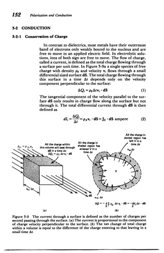
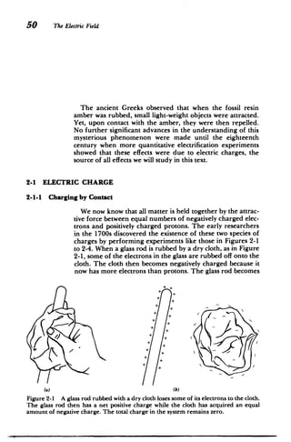
![Conduction 153
where the free current density of these charges Jf, is a vector
and is defined as
Jf = pfivi amp/M 2
(3)
If there is more than one type of charge carrier, the net
charge density is equal to the algebraic sum of all the charge
densities, while the net current density equals the vector sum
of the current densities due to each carrier:
Pf=lpf, JF=Xpfiv (4)
Thus, even if we have charge neutrality so that p =0, a net
current can flow if the charges move with different velocities.
For example, two oppositely charged carriers with densities
Pi = -P2 Po moving with respective velocities vl .and v2 have
P1 =PI+P2=0, J1 =pIvi+p 2 v2 =pO(vI-v 2) (5)
With vI 0 V2 a net current flows with zero net charge. This is
typical in metals where the electrons are free to flow while the
oppositely charged nuclei remain stationary.
The total current I, a scalar, flowing through a macroscopic
surface S, is then just the sum of the total differential currents
of all the charge carriers through each incremental size surface
element:
I=f J -dS (6)
Now consider the charge flow through the closed volume V
with surface S shown in Figure 3-9b. A time At later, that
charge within the volume near the surface with the velocity
component outward will leave the volume, while that charge
just outside the volume with a velocity component inward will
just enter the volume. The difference in total charge is
transported by the current:
AQ = fv [pf(t + At) -p(t)] dV
= pjiviAt - dS= - JAt - dS (7)
The minus sign on the right is necessary because when vi is in
the direction of dS, charge has left the volume so that the
enclosed charge decreases. Dividing (7) through by At and
taking the limit as At ->0, we use (3) to derive the integral
conservation of charge equation:
Jf j-dS+ LpdV = (8)
M](https://image.slidesharecdn.com/mitres6002s08part1-211102045902/85/Mitres-6-002_s08_part1-181-320.jpg)
![154 Polarizationand Conduction
Using the divergence theorem, the surface integral can be
converted to a volume integral:
[v[ j,+ p-] dV =0=>V - Jf+ =0 (9)
at at
where the differential point form is obtained since the
integral must be true for any volume so that the bracketed
term must be zero at each point. From Gauss's law (V - D =pr)
(8) and (9) can also be written as
Jf+L- dS=0, V - (jf + =La10
=
at(a) (10)
where j is termed the conduction current density and aD/at
is called the displacement current density.
This is the field form of Kirchoff's cirtuit current law that
the algebraic sum of currents at a node sum to zero. Equation
(10) equivalently tells us that the net flux of total current,
conduction plus displacement, is zero so that all the current
that enters a surface must leave it. The displacement current
does not involve any charge transport so that time-varying
current .can be transmitted through space without charge
carriers. Under static conditions, the displacement current is
zero.
3-2-2 Charged Gas Conduction Models
(a) Governing Equations.
In many materials, including good conductors like metals,
ionized gases, and electrolytic solutions as well as poorer
conductors like lossy insulators and semiconductors, the
charge carriers can be classically modeled as an ideal gas
within the medium, called a plasma. We assume that we have
two carriers of equal magnitude but opposite sign q with
respective masses m, and number densities n,. These charges
may be holes and electrons in a semiconductor, oppositely
charged ions in an electrolytic solution, or electrons and
nuclei in a metal. When an electric field is applied, the posi
tive charges move in the direction of the field while the
negative charges move in the opposite direction. These
charges collide with the host medium at respective frequen
cies v. and v-, which then act as a viscous or frictional dis
sipation opposing the motion. In addition to electrical and
frictional forces, the particles exert a force on themselves
through a pressure term due to thermal agitation that would
be present even if the particles were uncharged. For an ideal
gas the partial pressure p is
p = nkT Pascals [kg-s 2
-m'] (11)](https://image.slidesharecdn.com/mitres6002s08part1-211102045902/85/Mitres-6-002_s08_part1-182-320.jpg)
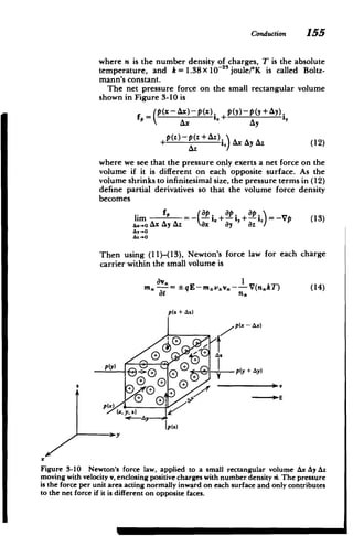
![156 Polarizationand Conduction
where the electric field E is due to the imposed field plus the
field generated by the charges, as given by Gauss's law.
(b) Drift-Diffusion Conduction
Because in many materials the collision frequencies are
typically on the order of x - 1013 Hz, the inertia terms in (14)
are often negligible. In this limit we can easily solve (14) for
the velocity of each carrier as
1 1
lim v,= qE--V(nkT)) (15)
av*I8MC. mVve n/
The charge and current density for each carrier are simply
given as
p* =qn,,, J =p'*
= qnav* (16)
Multiplying (15) by the charge densities then gives us the
constitutive law for each current as
J,=*qnsv,= pyE- DVp, (17)
where A, are called the particle mobilities and D. are their
diffusion coefficients
A* = q [A-kg I_-s
2
], D.= kT [m2
-s-'] (18)
assuming that the system is at constant temperature. We see
that the ratio D/s,: for each carrier is the same having units
of voltage, thus called the thermal voltage:
- -= volts [kg-m2
-A 1
-s ] (19)
IA q
This equality is known as Einstein's relation.
In equilibrium when the net current of each carrier is zero,
(17) can be written in terms of the potential as (E = -V V)
J+= J_.= 0 = -p siV V F D:Vps (20)
which can be rewritten as
V[ V+lnp] =0 (21)
The bracketed term can then only be a constant, so the charge
density is related to the potential by the Boltzmann dis
tribution:
p.= po eVIAT (22)
where we use the Einstein relation of (19) and po is the
equilibrium charge density of each carrier when V=0 and
are of equal magnitude because the system is initially neutral.](https://image.slidesharecdn.com/mitres6002s08part1-211102045902/85/Mitres-6-002_s08_part1-184-320.jpg)
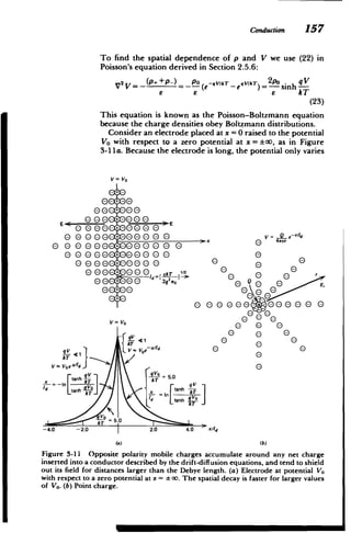
![158 Polarizationand Conduction
with the x coordinate so that (23) becomes
d2fl I qV 2 ekT
--
2 2-sinh V=0, V= -, l - (24)
dx lT kT 2poq
where we normalize the voltage to the thermal voltage k T/q
and ld is called the Debye length.
If (24) is multiplied by dVldx, it can be written as an exact
differential:
d 1d~ 2
hosh
d2
[(d) cosV]=0 (25)
dx 2dx da
The bracketed term must then be a constant that is evaluated
far from the electrode where the potential and electric field
E= -dV/dx are zero:
d2 V x>0
= - - (cosh F- sinh- (26)
dx LT Id 2 x<O
The different signs taken with the square root are necessary
because the electric field points in opposite directions on each
side of the electrode. The potential is then implicitly found by
direct integration as
tanh(V/4) e x>0
tanh(Vo/4) x<
The Debye length thus describes the characteristic length
over which the applied potential exerts influence. In many
materials the number density of carriers is easily of the order
of no= 102 0
/m 3
, so that at room temperature (T - 293*K), l is
typically 10 m.
Often the potentials are very small so that qV/k T< 1. Then,
the hyperbolic terms in (27), as well as in the governing
equation of (23), can be approximated by their arguments:
V2
V_- =0 (28)
This approximation is only valid when the potentials are
much less than the thermal voltage kT/q, which, at room
temperature is about 25 mv. In this limit the solution of (27)
shows that the voltage distribution decreases exponentially.
At higher values of Vo, the decay is faster, as shown in Figure
3-1 a.
If a point charge Q is inserted into the plasma medium, as
in Figure 3-11 b, the potential only depends on the radial
distance r. In the small potential limit, (28) in spherical coor
dinates is
I a ( 2 aV V
r2r Or 2=0 (29)](https://image.slidesharecdn.com/mitres6002s08part1-211102045902/85/Mitres-6-002_s08_part1-186-320.jpg)
![Conduction 159
Realizing that this equation can be rewritten as
02 (rV)
- (rV)- )=
1 (30)
we have a linear constant coefficient differential equation in
the variable (rV) for which solutions are
rV= A1 e~/ld+ A2 e+ld (31)
Because the potential must decay and not grow far from
the charge, A 2 =0 and the solution is
V= -d' (32)
47rer
where we evaluated A I by realizing that as r->0 the potential
must approach that of an isolated point charge. Note that for
small r the potential becomes very large and the small poten
tial approximation is violated.
(c) Ohm's Law
We have seen that the mobile charges in a system described
by the drift-diffusion equations accumulate near opposite
polarity charge and tend to shield out its effect for distances
larger than the Debye length. Because this distance is usually
so much smaller than the characteristic system dimensions,
most regions of space outside the Debye sheath are charge
neutral with equal amounts of positive and negative charge
density *po. In this region, the diffusion term in (17) is negli
gible because there are no charge density gradients. Then the
total current density is proportional to the electric field:
J = J+ +J_= po(v+-v-) = qno(iz++s-)E = -E (33)
where o [siemans/m (m-3 -kg~ -s
3
-A 2
)] is called the Ohmic
conductivity and (33) is the point form of Ohm's law. Some
times it is more convenient to work with the reciprocal
conductivity p, =(1/a-) (ohm-m) called the resistivity. We will
predominantly use Ohm's law to describe most media in this
text, but it is important to remember that it is often not valid
within the small Debye distances near charges. When Ohm's
law is valid, the net charge is zero, thus giving no contribution
to Gauss's law. Table 3-2 lists the Ohmic conductivities for
various materials. We see that different materials vary over
wide ranges in their ability to conduct charges.
The Ohmic conductivity of "perfect conductors" is large
and is idealized to be infinite. Since all physical currents in
(33) must remain finite, the electric field within the conductor](https://image.slidesharecdn.com/mitres6002s08part1-211102045902/85/Mitres-6-002_s08_part1-187-320.jpg)
![160 Polarizationand Conduction
is zero so that it imposes an equipotential surface:
E=o
limJ=o-E=> V=const (34)
J = finite
Table 3-2 The Ohmic conductivity
for various common substances at
room temperature
o- [siemen/m]
Silver" 6.3 x 10⁷
Copper" 5.9X 10⁷
Gold' 4.2 x 10⁷
Lead" 0.5 X 10⁷
Tin' 0.9X 10⁷
Zinc" 1.7 x 10⁷
Carbon" 7.3 x 10⁻⁴
Mercuryb 1.06 X 10⁶
Pure Water 4 x 10~
Nitrobenzeneb 5 x 10~
Methanolb 4 x 10⁵
Ethanolb 1.3 x 10
Hexane <Ix10
'From Handbook of Chemistry and Phy
sics, 49th ed., The Chemical Rubber Co.,
1968, p. E80.
b
From Lange's Handbook of Chemistry,
10th ed., McGraw-Hill, New York, 1961,
pp. 1220-21.
Throughout this text electrodes are generally assumed to
be perfectly conducting and thus are at a constant potential.
The external electric field must then be incident perpendic
ularly to the surface.
(d) Superconductors
One notable exception to Ohm's law is for superconducting
materials at cryogenic temperatures. Then, with collisions
negligible (v, =0) and the absolute temperature low (T - 0),
the electrical force on the charges is only balanced by their
inertia so that (14) becomes simply
-=* E (35)
at m*
We multiply (35) by the charge densities that we assume to be
constant so that the constitutive law relating the current](https://image.slidesharecdn.com/mitres6002s08part1-211102045902/85/Mitres-6-002_s08_part1-188-320.jpg)
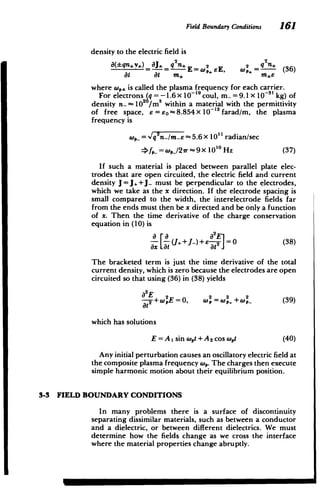
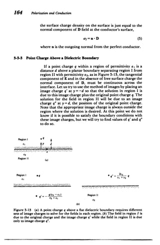
![Field Boundary Conditions 165
The potential in each region is
2 y O
V,2+(y d)2+z 2+(y+d)2+z2 II2),
I q (6)
2
4wE2 [x2
+(y -d) 2
+z 2
, y
with resultant electric field
E= -V V1
I (q~xi.+(y-d)i,+zi,] q'[xi +(y+d)i,+zi.I
4,rsE ( +(y --d)2+z2]3/2+ [2 +(y id) 2
+z2i3/2 ) (7)
q" (xi, +(y -d)i,+z i!
EI =-V VI = - 2 -Z9
4we 2 [x2 +(y-d)
2 +z2 I2
)
To satisfy the continuity of tangential electric field at y =0 we
have
E., =E.11 , ,,q
___ g- (8)
i 82
E 11
E. =
With no surface charge, the normal component of D must be
continuous at y = 0,
EIEj = e2 Ey1 => -q +q'= -q" (9)
Solving (8) and (9) for the unknown charges we find
(62-81)
81+82
21 2 (1 0)
(81+82)
The force on the point charge q is due only to the field
from image charge q':
qq I q2
(62-E1)
4 xle (2d)2 'L 16rE I(e I+ 92)d 2-,
3-3-4 Normal Component of P and soE
By integrating the flux of polarization over the same Gaus
sian pillbox surface, shown in Figure 3-12b, we relate the
discontinuity in normal component of polarization to the
surface polarization charge density o-, using the relations
M M](https://image.slidesharecdn.com/mitres6002s08part1-211102045902/85/Mitres-6-002_s08_part1-193-320.jpg)
![166 Polarizationand Conduction
from Section 3.1.2:
P-dS= - adS$P 2 -PIfl = -o-,n -(P 2 -P 1 )=-O-,
(12)
The minus sign in front of o-, results because of the minus sign
relating the volume polarization charge density to the diver
gence of P.
To summarize, polarization charge is the source of P, free
charge is the source of D, and the total charge is the source of
6oE. Using (4) and (12), the electric field interfacial dis
continuity is
n - (E2 -E i) - [(D2 -Di)-(P 2 -P)] af+o -, (13)
60 So
For linear dielectrics it is often convenient to lump polariza
tion effects into the permittivity e and never use the vector P,
only D and E.
For permanently polarized materials, it is usually con
venient to replace the polarization P by the equivalent
polarization volume charge density and surface charge
density of (12) and solve for E using the coulombic super
position integral of Section 2.3.2. In many dielectric prob
lems, there is no volume polarization charge, but at surfaces
of discontinuity a surface polarization charge is present as
given by (12).
EXAMPLE 3-2 CYLINDER PERMANENTLY POLARIZED ALONG ITS
AXIS
A cylinder of radius a and height L is centered about the z
axis and has a uniform polarization along its axis, P = Poi., as
shown in Figure 3-14. Find the electric field E and displace
ment vector D everywhere on its axis.
SOLUTION
With a constant polarization P, the volume polarization
charge density is zero:
P. = -V - P =0
Since P =0 outside the cylinder, the normal component of P
is discontinuous at the upper and lower surfaces yielding
uniform surface polarization charges:
o-,(z=L/2)=Po, o-p(z=-L12)=-Po](https://image.slidesharecdn.com/mitres6002s08part1-211102045902/85/Mitres-6-002_s08_part1-194-320.jpg)
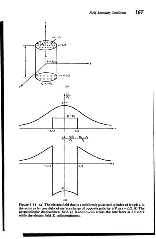
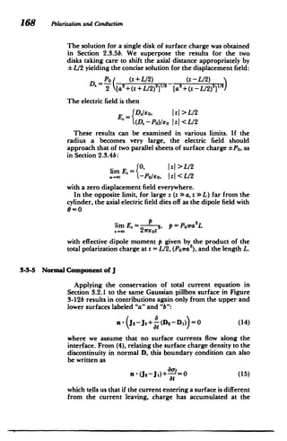
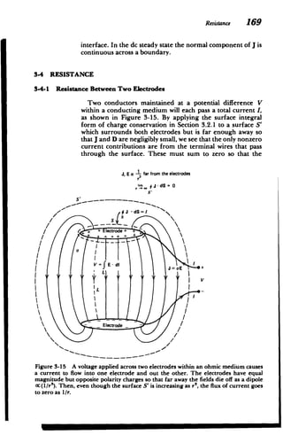
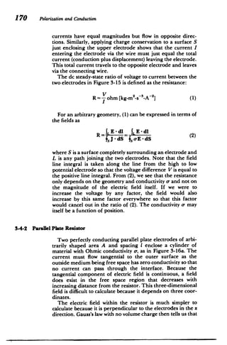
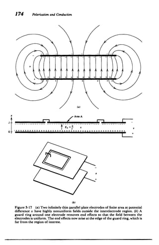
![Capacitance 175
the electrodes is as if the end effects were very far away and
not just near the electrode edges.
We often use the phrase "neglect fringing" to mean that the
nonuniform field effects near corners and edges are negli
gible.
With the neglect of fringing field effects near the electrode
ends, the electric field is perpendicular to the electrodes and
related to the voltage as
E. dx = v ->E. = v1 (1)
The displacement vector is then proportional to the electric
field terminating on each electrode with an equal magnitude
but opposite polarity surface charge density given by
D= eE= or(x = 0) = -of(x = 1) = evl (2)
The charge is positive where the voltage polarity is positive,
and vice versa, with the electric field directed from the posi
tive to negative electrode. The magnitude of total free charge
on each electrode is
qf= f(x =0)A =---v (3)
The capacitance C is defined as the magnitude of the ratio
of total free charge on either electrode to the voltage
difference between electrodes:
eA
C If
V I
(permittivity) (electrode area) farad [A2
S4 -kg- -2]
spacing
(4)
Even though the system remains neutral, mobile electrons on
the lower electrode are transported through the voltage
source to the upper electrode in order to terminate the dis
placement field at the electrode surfaces, thus keeping the
fields zero inside the conductors. Note that no charge is
transported through free space. The charge transport
between electrodes is due to work by the voltage source and
results in energy stored in the electric field.
In SI units, typical capacitance values are very small. If the
2
electrodes have an area of A = 1cm2
(10- iM ) with spacing of
1 = 1 mm (10- im), the free space capacitance is C-
0.9x 10⁻¹² farad. For this reason usual capacitance values are
expressed in microfarads (1 U f = 10-6 farad), nanofarads
(1 nf = 10-9 farad), and picofarads (1 pf = 10-' farad).](https://image.slidesharecdn.com/mitres6002s08part1-211102045902/85/Mitres-6-002_s08_part1-203-320.jpg)
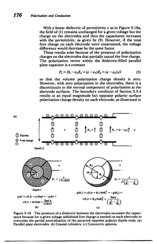
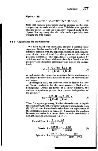
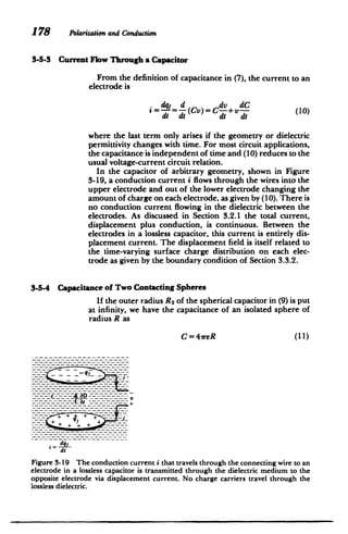
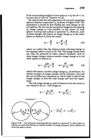
![Lossy Media 181
The capacitance is then given as the ratio of the total charge
on the two spheres to the voltage,
2 1 q. _~
.C "= 2Q * -1) 2Q
,
Vo Vo n-1 n Vo
=8reR In 2 (24)
where we recognize the infinite series to be the Taylor series
expansion of In (1 + x) with x = 1. The capacitance of two
contacting spheres is thus 2 In 2 1.39 times the capacitance
of a single sphere given by (11).
The distance from the center to each image charge is
obtained from (23) substituted into (15) as
=((- 1)" (n + 1)(n-)
bn= ( )R+
1
2R = (-i)R (25)
n(-1) n
We find the force of attraction between the spheres by
taking the sum of the forces on each image charge on one of
the spheres due to all the image charges on the other sphere.
The force on the nth image charge on one sphere due to the
mth image charge in the other sphere is
-qq. -Q_(-_)"_'" nm
fn= -7- -n (26)
41re[2R bbM]2
4weR (m+n)
where we used (23) and (25). The total force on the left
sphere is then found by summing over all values of m and n,
0 *o -Q 00 * (_-I)"+'nm
f = I Y_ fnm= _2 + M)s
m=1n=1 4reR m=, n=- (n+m)
-QE 1
6 [ln 2
- - (27)
SR
4
where the double series can be explicitly expressed.* The
force is negative because the like charge spheres repel each
other. If Qo = 1 coul with R = 1 m, in free space this force is
f-6.6x 10⁸ nt, which can lift a mass in the earth's gravity
field of 6.8 x 10⁷ kg (-3 x 10⁷ lb).
3-6 LOSSY MEDIA
Many materials are described by both a constant permit
tivity e and constant Ohmic conductivity o-. When such a
material is placed between electrodes do we have a capacitor
* See Albert D. Wheelon, Tables of Summable Series and Integrals Involving Bessel
Functions, Holden Day, (1968) pp. 55, 56.](https://image.slidesharecdn.com/mitres6002s08part1-211102045902/85/Mitres-6-002_s08_part1-209-320.jpg)
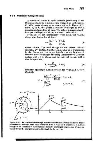
![186 PoLarizationand Conduction
is infinite (an impulse) as the displacement field instan
taneously changes from zero to (13) to produce the surface
charge on each electrode:
of(x=0)=-f(x =a+b)=D. (14)
After the voltage has been on a long time, the fields
approach their steady-state values, as in Figure 3-22b.
Because there are no more time variations, the current
density must be continuous across the interface just the same
as for two series resistors independent of the permittivities,
J.(t- oo) = a-IEI= o-2E 2 = 0102 V (15)
o2a +otb
where we again used (12). The interfacial surface charge is
now
oyf(x = a)= 62E2-s.EI = (E20'1-s 10'2)V (16)
or2a+o-
1b
What we have shown is that for early times the system is
purely capacitive, while for long times the system is purely
resistive. The inbetween transient interval is found by using
(12) with charge conservation applied at the interface:
nJ2-J,+ d(D2 -DI) =0
d
=o 2E2 - -EI+ d[E2
E 2- 1EI]=0 (17)
dt
With (12) to relate E2 to El we obtain a single ordinary
differential equation in EI,
dE 1 E1 cr2V
dI+-= 0' (18)
dt r 92a+E1b
where the relaxation time is a weighted average of relaxation
times of each material:
Ey=b+ 2a (19)
a- b + o-2a
Using the initial condition of (13) the solutions for the fields
are
EI= 0'2 V (1-e )+ V ,--1,
-2a+o-b E2a+elb (20)
E2= (1-e~)+ e-
o-
2a+ -ib 62a+Elb](https://image.slidesharecdn.com/mitres6002s08part1-211102045902/85/Mitres-6-002_s08_part1-214-320.jpg)
![Lossy Media 187
Note that as t ->0 the solutions approach those of (15). The
interfacial surface charge is
of(x =a)=e 2E2- eE1=(62i -1 '2) (1-e"')V (21)
o-2a+a-,b
which is zero at t = 0 and agrees with (16) for t -> 0.
The total current delivered by the voltage source is
( dE
dE1
i-E -+e
-Id= 0-2E2+E2 -) Id
di di)
Lo-a +u- b T) ' e2a+eib o-2a+o-1b)
+ EIE2 8(t) IdV (22)
e2 a +eib J
where the last term is the impulse current that instan
taneously puts charge on each electrode in zero time at t =0:
0(,) -50
>f 0'8(t) dt = I
100, t=01
To reiterate, we see that for early times the capacitances
dominate and that in the steady state the resistances dominate
with the transition time depending on the relaxation times
and geometry of each region. The equivalent circuit for the
system is shown in Figure 3-22c as a series combination of a
parallel resistor-capacitor for each region.
(b) Open Circuit
Once the system is in the dc steady state, we instantaneously
open the circuit so that the terminal current is zero. Then,
using (22) with i =0, we see that the fields decay indepen
dently in each region with the relaxation time of each region:
E-2V 81
61
c-2a+o-ib
El =2 02 +(23)
a-2 a+o1 b -2
The open circuit voltage and interfacial charge then decay as
V. =Ela+E
2 b= [o-2ae_"I +o-ibe~"'2]
o-2a +e-1b
(24)
oy e 2E2 --
e 1E [20-1 e --
(
= t/2 -eio2e~
a-2a + o 1b](https://image.slidesharecdn.com/mitres6002s08part1-211102045902/85/Mitres-6-002_s08_part1-215-320.jpg)
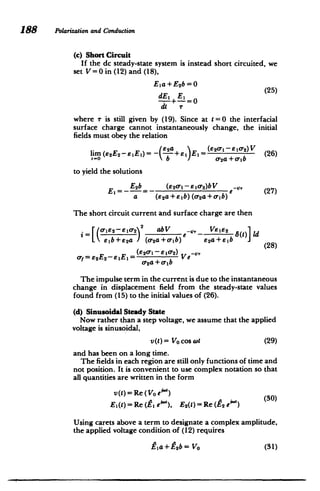
![Lossy Media 189
while the interfacial charge conservation equation of (17)
becomes
-2 2- 0 1 +)( (62 4 2- e 1E1 ) = [0-2+j06 2 ]E2
- [ 1 +jWuEi1=0 (32)
The solutions are
Z1 F2 Vo
ElE2V0 -(33)
(wE 2+o- 2) j6)1+0-1) [b(o+jwe)+a(- 2+jWe 2)]
which gives the interfacial surface charge amplitude as
= e2E2-eE = (34)
[b(a1 +jw i)+a(a-
2+jWs 2)]
As the frequency becomes much larger than the reciprocal
relaxation times,
(0 a -, a 2 35)
8i2
the surface charge density goes to zero. This is because the
surface charge cannot keep pace with the high-frequency
alternations, and thus the capacitive component dominates.
Thus, in experimental work charge accumulations can be
prevented if the excitation frequencies are much faster than
the reciprocal charge-relaxation times.
The total current through the electrodes is
I =(-1 + jwEI)Eild= (o2 +jWe 2)E2ld
2+jWe
ld(o1+jwe 1) (o- 2
)Vo
[b(o-i +jwj)+a(o- 2+jW'2)]
V0
(36)
R2
R2C2jW+1 R 1Cijw+1
with the last result easily obtained from the equivalent circuit
in Figure 3-22c.
3-6-4 Distributed Systems
(a) Governing Equations
In all our discussions we have assumed that the electrodes
are perfectly conducting so that they have no resistance and
the electric field terminates perpendicularly. Consider now
the parallel plate geometry shown in Figure 3-23a, where the
electrodes have a large but finite conductivity a-,. The elec
trodes are no longer equi-potential surfaces since as the cur
rent passes along the conductor an Ohmic iR drop results.](https://image.slidesharecdn.com/mitres6002s08part1-211102045902/85/Mitres-6-002_s08_part1-217-320.jpg)
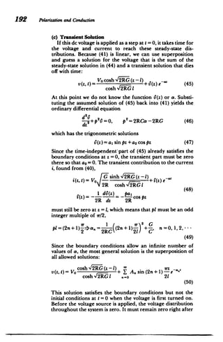
![Lossy Media 193
being turned on otherwise the time derivative in (40) would
be infinite, which requires nonphysical infinite currents. Thus
we impose the initial condition
cosh - 2_RG(z - 1) -wz
v(z, t = 0)=hl= VO+ Y An sin (2n+1)
cosh,/lIR1 '.o 21
(51)
We can solve for the amplitudes A. by multiplying (51)
through by sin (2m+1) rz/21 and then integrating over z
from 0 to 1:
cosh f2iRG(z-1)sin (2m+1)"dz
cosh %/2RG o 21
1 0 7Z iTz
+J Asin(2n+1) sin(2m+1) -dz (52)
1) jsin(21 21
The first term is easily integrated by writing the hyperbolic
cosine in terms of exponentials,* while the last term integrates
to zero for all values of m not equal to n so that the ampli
tudes are
An = rVO(2n+1) 2 (53)
7 2RG +[(2n +1) w/2]
The total solutions are then
v(z' t) Vo cosh l2iER (z -1)
cosh %Iv'- I
(2n + 1) sin [(2n + 1) (lrz/21)]e-*-'
12 V,=o 2RG+[(2n+1)(r/2)] 2
i(z, t)= 1 av
2R az
Vo G/2R sinh
V' (z-1) (54)
cosh N/IER I
r2
Vo (2n + 1)2 cos [(2n + 1) (irz/2I)] e--'
4lR .=1 2RG+[(2n + 1) (1r21)]2
*Jcosh a(z - 1) sin bz dz
=a2+b,[a sin bz sinh a(z -L)- b cos bz cosh a(z - 1)]
)bz sin (2m+ 1)bz dz = 0 m n
Ssin (2n+
11/2 m=n](https://image.slidesharecdn.com/mitres6002s08part1-211102045902/85/Mitres-6-002_s08_part1-221-320.jpg)
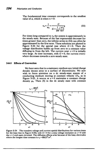
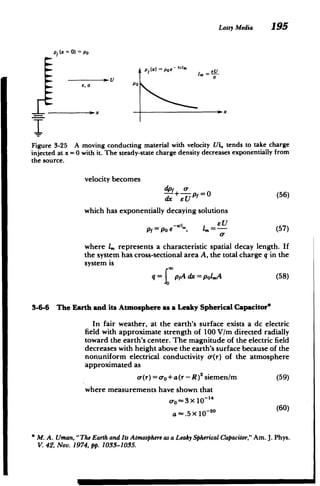
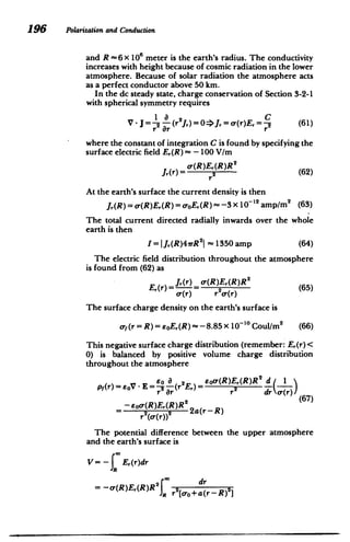
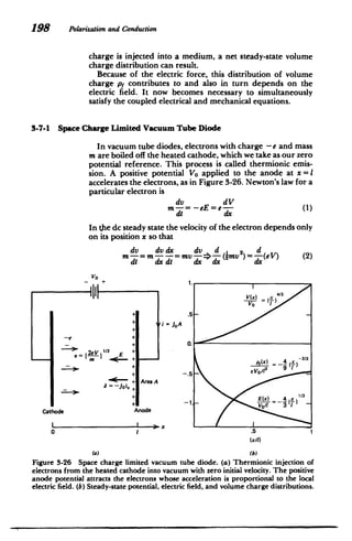
![Field-dependentSpace Charge Distributions 199
With this last equality, we have derived the energy conser
vation theorem
[x -eV=const (3)
DMV-eV]=0>bM
where we say that the kinetic energy 2mv
2 plus the potential
energy -eV is the constant total energy. We limit ourselves
here to the simplest case where the injected charge at the
cathode starts out with zero velocity. Since the potential is also
chosen to be zero at the cathode, the constant in (3) is zero.
The velocity is then related to the electric potential as
= (2e V)" 2 (4)
In the time-independent steady state the current density is
constant,
-g=0=>J= -JOi. (5)
dx
and is related to the charge density and velocity as
In1/2
2
Jo= -pfj Jp'f= -Joy) V 1 (6)
Note that the current flows from anode to cathode, and
thus is in the negative x direction. This minus sign is
incorporated in (5) and (6) so that Jo is positive. Poisson's
equation then requires that
V 1 V
-f > 2V=Jo 'n1/2v-/(7
= 6' (Fe) V-E
Power law solutions to this nonlinear differential equation are
guessed of the form
V = Bxt' (8)
which when substituted into (7) yields
Bp(p - )x0-2=J (;1) B -12-02 (9)
6 e)
For this assumed solution to hold for all x we require that
p 4
P -2= -- >p =- 4(10)
2 3
which then gives us the amplitude B as
B= - - )- (11)](https://image.slidesharecdn.com/mitres6002s08part1-211102045902/85/Mitres-6-002_s08_part1-227-320.jpg)
![Field-dependentSpace ChargeDistributions 201
The charge transit time r between electrodes is found by
solving (18) with x = 1:
( 1/2
T=31 -(19)
2e Vo)
For an electron (m = 9.1 X 10~3' kg, e = 1.6x 10 '9
coul) with
100 volts applied across = 1cm (10~2 m) this time is r
5 X 10⁻⁹ sec. The peak electron velocity when it reaches the
anode is v(x = l)~6x 0 m/sec, which is approximately 50
times less than the vacuum speed of light.
Because of these fast response times vacuum tube diodes
are used in alternating voltage applications for rectification as
current only flows when the anode is positive and as
nonlinear circuit elements because of the three-halves power
law of (13) relating current and voltage.
3-7-2 Space Charge Limited Conduction in Dielectrics
Conduction properties of dielectrics are often examined by
injecting charge. In Figure 3-27, an electron beam with cur
rent density J = -Joi, is suddenly turned on at t = 0.* In media,
the acceleration of the charge is no longer proportional to the
electric field. Rather, collisions with the medium introduce a
frictional drag so that the velocity is proportional to the elec
tric field through the electron mobility /A:
v =-AE (20)
As the electrons penetrate the dielectric, the space charge
front is a distance s from the interface where (20) gives us
ds/dt = -- E(s) (21)
Although the charge density is nonuniformly distributed
behind the wavefront, the total charge Q within the dielectric
behind the wave front at time t is related to the current
density as
JoA = pfpE.A = -Qlt =>Q -JoAt (22)
Gauss's law applied to the rectangular surface enclosing all
the charge within the dielectric then relates the fields at the
interface and the charge front to this charge as
SE - dS= (eE(s)-soE(0)]A = Q = -JoAt (23)
* See P. K. Watson, J. M. Schneider, andH. R. Till, Electrohydrodynamic Stabilityof Space
Charge Limited Currents In Dielectric Liquids. II. ExperimentalStudy, Phys. Fluids 13
(1970), p. 1955.](https://image.slidesharecdn.com/mitres6002s08part1-211102045902/85/Mitres-6-002_s08_part1-229-320.jpg)
![202 Polarization and Conduction
Electron beam
J = -- joio
cdtion:. imi te Surface of integration for Gauss's
o law: feE(s)-e0 E(0)]A=Q=-JOAt
0 .... .. =.
V~t)............ M ii ]
e, Pt = 0 E +.4 Moving space charge front
+
ds = -gEls)
L 7IElectrode area A
I E
(a)
X
1
.
'(x - 312
1ot
2
VO
~2e
P/ =0
2
.. Io'1122
xl1 .5 1- 0.
-(=-2I
)
E (x) __ x_1/2
Eep---- VO/1 2 1
E. =--{2J x 112
-
5-
PAX) 3 -X
EV,/112
0.5 1.0
1/o2 t 1
112
-1.
.5
(x/l)
(b) (c)
Figure 3-27 (a) An electron beam carrying a current -Joi. is turned on at t = 0. The
electrons travel through the dielectric with mobility p. (b) The space charge front, at a
distance s in front of the space charge limited interface at x =0, travels towards the
opposite electrode. (c) After the transit time t, = [2eLIMJo]11
' the steady-state potential,
electric field, and space charge distributions.
The maximum current flows when E(O) =0, which is called
space charge limited conduction. Then using (23) in (21)
gives us the time dependence of the space charge front:
ds yJot yLJot
2
-=- -*s(t)= (24)
dt e 2e
Behind the front Gauss's law requires
dE- P= Jo dE. Jo
(25)
dx e eE. x dx ey.](https://image.slidesharecdn.com/mitres6002s08part1-211102045902/85/Mitres-6-002_s08_part1-230-320.jpg)
![EnergyStored in a Dielectric Medium 205
where we recognize that each bracketed term is just the
potential at the final position of each charge and includes
contributions from all the other charges, except the one
located at the position where the potential is being evaluated:
W=2[q 1 V1 +q 2 V2 +q 3 V3 ] (3)
Extending this result for any number N of already existing
free point charges yields
I IV
W =- E, q.V (4)
2n=1
The factor of - arises because the potential of a point charge
at the time it is brought in from infinity is less than the final
potential when all the charges are assembled.
(b) Binding Energy of a Crystal
One major application of (4) is in computing the largest
contribution to the binding energy of ionic crystals, such as
salt (NaCI), which is known as the Madelung electrostatic
energy. We take a simple one-dimensional model of a crystal
consisting of an infinitely long string of alternating polarity
point charges q a distance a apart, as in Figure 3-29. The
average work necessary to bring a positive charge as shown in
Figure 3-29 from infinity to its position on the line is obtained
from (4) as
1 2q 2
I11 11 I
W= -+--- ----- --- (5)
2 47rea 2 3 4 5 6
The extra factor of 2 in the numerator is necessary because
the string extends to infinity on each side. The infinite series
is recognized as the Taylor series expansion of the logarithm
2 3 4 5
In (I+x)= x +---+ (6)
2 3 4 5
((6
+q
+q -q +q -q +q -4 -q +q -q +q -q +q
<- a--)I
Figure 3-29 A one-dimensional crystal with alternating polarity charges q a dis
tance a apart.](https://image.slidesharecdn.com/mitres6002s08part1-211102045902/85/Mitres-6-002_s08_part1-233-320.jpg)
![206 Polarizationand Conduction
where x = I so that*
W= In 2 (7)
41rea
This work is negative because the crystal pulls on the charge
as it is brought in from infinity. This means that it would take
positive work to remove the charge as it is bound to the
crystal. A typical ion spacing is about 3 A (3 x 101' m) so that
if q is a single proton (q= 1.6x 10- 19
coul), the bindingenergy
is W- 5.3 x 10O' joule. Since this number is so small it is
usually more convenient to work with units of energy per unit
electronic charge called electron volts (ev), which are obtained
by dividing W by the charge on an electron so that, in this
case, W-3.3 ev.
If the crystal was placed in a medium with higher permit
tivity, we see from (7) that the binding energy decreases. This
is why many crystals are soluble in water, which has a relative
dielectric constant of about 80.
3-8-2 Work Necessary to Form a Continuous Charge Distribution
Not included in (4) is the self-energy of each charge itself
or, equivalently, the work necessary to assemble each point
charge. Since the potential V from a point charge q is pro
portional to q, the self-energy is proportional q2
. However,
evaluating the self-energy of a point charge is difficult
because the potential is infinite at the point charge.
To understand the self-energy concept better it helps to
model a point charge as a small uniformly charged spherical
volume of radius R with total charge Q = shrRpo. We assem
ble the sphere of charge from spherical shells, as shown in
Figure 3-30, each of thickness dr. and incremental charge
dq. = 41rr. drpo. As we bring in the nth shell to be placed at
radius r. the total charge already present and the potential
there are
4 3 . q. r2p
q.V=-rrpo, = r 3 (8)
* Strictly speaking, this seriesis only conditionallyconvergentforx = 1 anditssum depends on
the groupingof individual terms. If the seriesin (6) for x = 1 is rewrittenas
1 1 111 1 1 1
2 4 3 6 8 2k-1 4k-2 4k
then itssum is 2 In 2. [See J. Pleinesand S. Mahajan,On ConditionallyDivergentSeriesand
a PointChargeBetween Two ParallelGrounded Planes,Am. J. Phys. 45 (1977) p. 868.]](https://image.slidesharecdn.com/mitres6002s08part1-211102045902/85/Mitres-6-002_s08_part1-234-320.jpg)
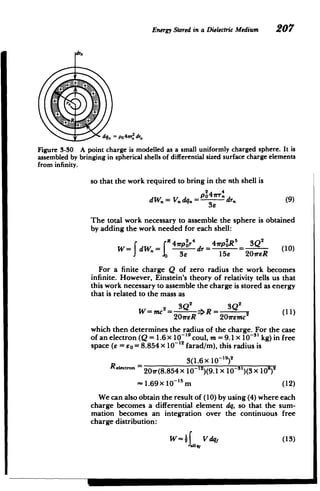
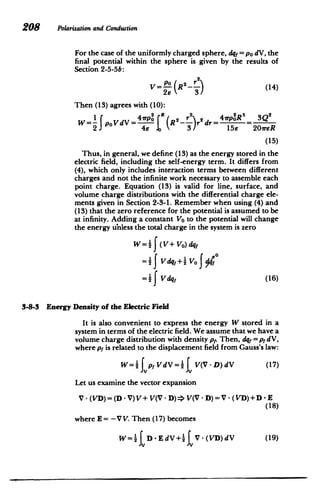
![Energy Stored in a Dielectric Medium 209
The last term on the right-hand side can be converted to a
surface integral using the divergence theorem:
(20)
fVD-dS
t V-(VD)dV=
If we let the volume V be of infinite extent so that the enclos
ing surface S is at infinity, the charge distribution that only
extends over a finite volume looks like a point charge for
which the potential decreases as 1/r and the displacement
vector dies off as I/r2
. Thus the term, VD at best dies off as
1/re. Then, even though the surface area of S increases as r
2
the surface integral tends to zero as r becomes infinite as /r.
Thus, the second volume integral in (19) approaches zero:
lim V -(VD)dV = VD-dS=0 (21)
This conclusion is not true if the charge distribution is of
infinite extent, since for the case of an infinitely long line or
surface charge, the potential itself becomes infinite at infinity
because the total charge on the line or surface is infinite.
However, for finite size charge distributions, which is always
the case in reality, (19) becomes
W=2space D-EdV
= 1eE dV (22)
all space
where the integration extends over all space. This result is
true even if the permittivity e is a function of position. It is
convenient to define the energy density as the positive-
definite quantity:
W . 2 3 2
w =2
1 E joule/m [kg-m -s ] (23)
where the total energy is
W= space wdV (24)
Note that although (22) is numerically equal to (13), (22)
implies that electric energy exists in those regions where a
nonzero electric field exists even if no charge is present in that
region, while (13) implies that electric energy exists only
where the charge is nonzero. The answer as to where the
energy is stored-in the charge distribution or in the electric
field-is a matter of convenience since you cannot have one
without the other. Numerically both equations yield the same
answers but with contributions from different regions of
space.](https://image.slidesharecdn.com/mitres6002s08part1-211102045902/85/Mitres-6-002_s08_part1-237-320.jpg)
![_ - - - -
-
~
-
~ ~
Energy Stored in a DielectricMedium 211
(c) Binding Energy of an Atom
In Section 3-1-4 we modeled an atom as a fixed positive
point charge nucleus Q with a surrounding uniform spheri
cal cloud of negative charge with total charge -Q, as in
Figure 3-31. Potentials due to the positive point and negative
volume charges are found from Section 2-5-5b as
V,(r) = Q
41reor
3Q 2r 2
- 3 (R--, r<R
81reoRS 3
V_(r) =
Q , r>R (30)
41reor
The binding energy of the atom is easily found by super
position considering first the uniformly charged negative
sphere with self-energy given in (10), (15), and (26) and then
adding the energy of the positive point charge:
3Q2
9___
W= 3Q2+Q[ V-(r = 0)] = - Q2 (31)
20rsoR 40ireoR
This is the work necessary to assemble the atom from
charges at infinity. Once the positive nucleus is in place, it
attracts the following negative charges so that the field does
work on the charges and the work of assembly in (31) is
negative. Equivalently, the magnitude of (31) is the work
necessary for us to disassemble the atom by overcoming the
attractive coulombic forces between the opposite polarity
charges.
When alternatively using (4) and (13), we only include the
potential of the negative volume charge at r = 0 acting on the
positive charge, while we include the total potential due to
both in evaluating the energy of the volume charge. We do
Total negative
charge - Q
V(r) = 3Q(R
2
_r2/3)
4reor BweoR 3
~ ~ ~~E--~_r <R
~ 4 - ,Q
-
2 3
r
4veor 4reOR
Figure 3-31 An atom can be modelled as a point charge Q representing the nucleus,
surrounded by a cloud of uniformly distributed electrons with total charge - Q within
a sphere of radius R.](https://image.slidesharecdn.com/mitres6002s08part1-211102045902/85/Mitres-6-002_s08_part1-239-320.jpg)
![212 Polarizationand Conduction
not consider the infinite self-energy of the point charge that
would be included if we used (22):
W=jQV_(r=0)-21 [V(r)+V-(r)]irk-dr
2 3Q r -3r2+ r4)dr =- -
l6vrEoR 8reoRg 2 R 2R
=- 4 (32)
40ireoR
3-8-5 Energy Stored in a Capacitor
In a capacitor all the charge resides on the electrodes as a
surface charge. Consider two electrodes at voltage V1 and V2
with respect to infinity, and thus at voltage difference V=
V2 - V1, as shown in Figure 3-32. Each electrode carries
opposite polarity charge with magnitude Q. Then (13) can be
used to compute the total energy stored as
W =[f Vo. dS1+ V20-
2 dS2 (33)
J2
Since each surface is an equipotential, the voltages V, and V2
may be taken outside the integrals. The integral then reduces
to the total charge Q on each electrode:
w=[VIJ
1 _1 dS1+V2 0- dS2
-Q Q
= (V2 - V1)Q= QV (34)
S2
Fiue33. Acpcto trs.nryi teeet.cfed
WV QV= CV2 Q2C
S-2 s2](https://image.slidesharecdn.com/mitres6002s08part1-211102045902/85/Mitres-6-002_s08_part1-240-320.jpg)
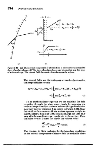
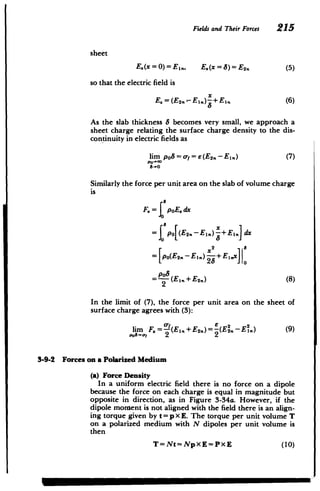
![216 Polarizationand Conduction
y
+q
d +q E(r + d) F =q[E(r + d) - E(0r
d (qd -V) E(r)
(p .V)E(r)
F_ -- E r+d E(r)
F=F +F =0 r -q
t=dxF =qdxE =pxE
Unifprm field Nonuniform field
(a) (b)
Figure 3-34 (a) A torque is felt by a dipole if its moment is not aligned with the
electric field. In a uniform electric field there is no net force on a dipole because the
force on each charge is equal in magnitude but opposite in direction. (b) There is a net
force on a dipole only in a nonuniform field.
For a linear dielectric, this torque is zero because the
polarization is induced by the field so that P and E are in the
same direction.
A net force can be applied to a dipole if the electric field is
different on each end, as in Figure 3-34b:
f = -q[E(r)-E(r+d)] (11)
For point dipoles, the dipole spacing d is very small so that the
electric field at r + d can be expanded in a Taylor series as
E(r + d) -E(r) + d- aE(r) +d, a E(r) +d. aE(r)
ax ay az
= E(r)+(d - V)E(r) (12)
Then the force on a point dipole is
f = (qd - V)E(r)= (p - V)E(r) (13)
If we have a distribution of such dipoles with number
density N, the polarization force density is
F= Nf= (Np - V)E = (P - V)E (14)
Of course, if there is any free charge present we must also
add the coulombic force density p1E.
(b) Permanently Polarized Medium
A permanently polarized material with polarization Poi, is
free to slide between parallel plate electrodes, as is shown in
Figure 3-35.](https://image.slidesharecdn.com/mitres6002s08part1-211102045902/85/Mitres-6-002_s08_part1-244-320.jpg)
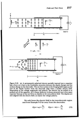
![-
=
Z
2
8
Fields and Their Forces 219
arises, as in Figure 3-35b. The dipoles tend to line up as
shown with the positive ends attracted towards the negative
electrode and the negative dipole ends towards the positive
electrode. Because the farther ends of the dipoles are in a
slightly weaker field, there is a net force to the right tending
to draw the dielectric into the capacitor.
The force density of (14) is
=. E. + , E. EY E 20
F.= P +P,- -- O) E.- E,- (20)
ax ay ax ay
Because the electric field is curl free, as given in (16), the
force density is further simplified to
(E-EO) aE22)
F.= - (E +E) (21)
2 ax
The total force is obtained by integrating (21) over the
volume of the dielectric:
fx - EE E+)dx
(j(E dy dz
7
(e eo)sd (E 2+ 1 E ()- EO) V(2d
2 - (22)
2 (E! +E,)I,,-M-
where we knew that the fields were zero at x = -co and uni
form at x = xo:
E,(xo) = Vo/s, E.(xo)= 0 (23)
The force is now independent of voltage polarity and always
acts in the direction to pull the dielectric into the capacitor if
6 >60.
3-9-3 Forces on a Capacitor
Consider a capacitor that has one part that can move in the
x direction so that the capacitance depends on the coordinate
x:
q =C(x)v (24)
The current is obtained by differentiating the charge with
respect to time:
.dq d dv dC(x)
= = d[C(x)v] = C(x) d-+ V di
dv dC(x)dx (25)
dt dx d(](https://image.slidesharecdn.com/mitres6002s08part1-211102045902/85/Mitres-6-002_s08_part1-247-320.jpg)
![220 Polarizationand Conduction
Note that this relation has an extra term over the usual circuit
formula, proportional to the speed of the moveable member,
where we expanded the time derivative of the capacitance by
the chain rule of differentiation. Of course, if the geometry is
fixed and does not change with time (dx/dt = 0), then (25)
reduces to the usual circuit expression. The last term is due to
the electro-mechanical coupling.
The power delivered to a time-dependent capacitance is
d
p=vi=v [C(x)v] (26)
dt
which can be expanded to the form
d 1 2 dC(x)
P = [DC(x)V ]+iv dt
d 1 , dC(x) dx
= [CQx)v I+tv (27)
di d dt
where the last term is again obtained using the chain rule of
differentiation. This expression can be put in the form
dW dx
P =-d+fx - (28)
di dt
where we identify the power p delivered to the capacitor as
going into increasing the energy storage W and mechanical
power fdxldt in moving a part of the capacitor:
W=C(x)V, 12 dC(x) (29)
W=4Cx~v, f~4v2
dx
Using (24), the stored energy and force can also be ex
pressed in terms of the charge as
1 q 2
1 q2
dC(x) 1 2d[LIC(x)]
W=--f.=- =g
2C(x)' 2 C2(x) dx dx
(30)
To illustrate the ease in using (29) or (30) to find the force,
consider again the partially inserted dielectric in Figure
3-35b. The capacitance when the dielectric extends a distance
x into the electrodes is
exd (1-x)d (31)
C(x)-+so (1
S S
so that the force on the dielectric given by (29) agrees with
(22):
1 2 dC(x) = ) Vod
f.= 0 - = e-eo) s (32)
dx s](https://image.slidesharecdn.com/mitres6002s08part1-211102045902/85/Mitres-6-002_s08_part1-248-320.jpg)
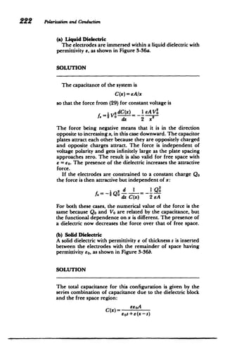
![ElectrostaticGenerators 223
The force on the upper electrode for constant voltage is
I 2 d e2oAVo
f. = i -C)- s1
dx 2[eos +e(x -s)]
If the electrode just rests on the dielectric so that x = s, the
force is
62A2O
e AVo
2sos
This result differs from that of part (a) when x = s by the
factor s,= e/eo because in this case moving the electrode even
slightly off the dielectric leaves a free space region in between.
In part (a) no free space gap develops as the liquid dielectric
fills in the region, so that the dielectric is always in contact
with the electrode. The total force on the electrode-dielectric
interface is due to both free and polarization charge.
With the electrodes constrained to constant charge, the
force on the upper electrode is independent of position and
also independent of the permittivity of the dielectric block:
sd 1 1 Q2
2Q 0dx C(x) 2 eoA
3-10 ELECTROSTATIC GENERATORS
3-10-1 Van de Graaff Generator
In the 1930s, reliable means of generating high voltages
were necessary to accelerate charged particles in atomic
studies. In 1931, Van de Graaff developed an electrostatic
generator where charge is sprayed onto an insulating moving
belt that transports this charge onto a conducting dome, as
illustrated in Figure 3-37a. If the dome was considered an
isolated sphere of radius R, the capacitance is given as C =
4reoR. The transported charge acts as a current source feed
ing this capacitance, as in Figure 3-37b, so that the dome
voltage builds up linearly with time:
dv i
=C =>v=-t(1)
dt C
This voltage increases until the breakdown strength of the
surrounding atmosphere is reached, whereupon a spark dis
charge occurs. In air, the electric field breakdown strength Eb
is 3 X 10⁶ V/m. The field near the dome varies as E,= VR/r2
,
which is maximum at r= R, which implies a maximum voltage
of Vmax= ER. For Vmax = 10 V, the radius of the sphere](https://image.slidesharecdn.com/mitres6002s08part1-211102045902/85/Mitres-6-002_s08_part1-251-320.jpg)
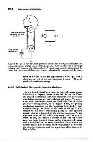
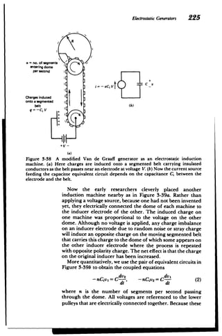
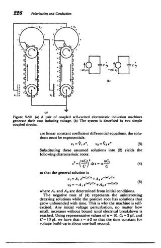
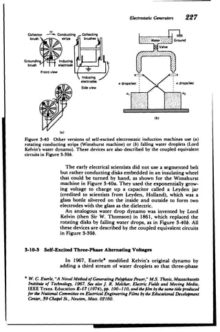
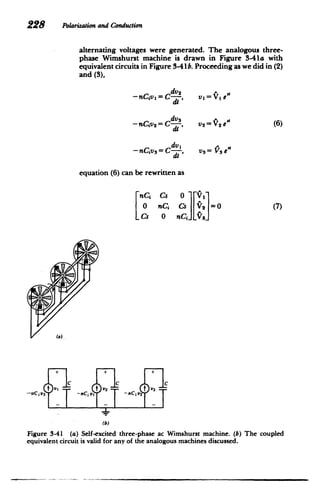
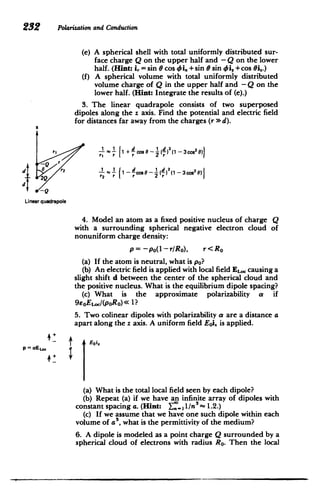
![Problems 23
field EL, differs from the applied field E by the field due to
the dipole itself. Since Edi varies within the spherical cloud,
we use the average field within the sphere.
d
(a) Using the center of the cloud as the origin, show that
the dipole electric field within the cloud is
- Qri, Q(ri.-di])
47reoRo +47rE[d+r2-2rd cos
(b) Show that the average x and y field components are
zero. (Hint: i, = sin 0 cos i. +sin 0 sin i, +cos 0i..)
(c) What is the average z component of the field?
(Hint: Change variables to u = r+d - 2rd cos 9 and
remember (r -d) 2
=Ir - d.)
(d) If we have one dipole within every volume of IIrR,
how is the polarization P related to the applied field E?
7. Assume that in the dipole model of Figure 3-5a the mass
of the positive charge is so large that only the election cloud
moves as a solid mass m.
(a) The local electric field is E0 .What is the dipole spacing?
(b) At t = 0, the local field is turned off (Eo = 0). What is the
subsequent motion of the electron cloud?
(c) What is the oscillation frequencg if Q has the charge
and mass of an electron with Ro = 10-1 m?
(d) In a real system there is always some damping that we
take to be proportional to the velocity (fdapin, = - 0v). What
is the equation of motion of the electron cloud for a sinusoi
dal electric field Re(toe""')?
(e) Writing the driven displacement of the dipole as
d = Re(deW').
what is the complex polarizability d, where # = Qd = SEo?
(f) What is the complex dielectric constant 6= , +jej of
the system? (Hint: Define 4o = Q2
N/(meo).)
(g) Such a dielectric is placed between parallel plate elec
trodes. Show that the equivalent circuit is a series R, L, C
shunted by a capacitor. What are C1, Cs, L, and R?
(h) Consider the limit where the electron cloud has no
mass (m = 0). With the frequency w as a parameter show that](https://image.slidesharecdn.com/mitres6002s08part1-211102045902/85/Mitres-6-002_s08_part1-261-320.jpg)
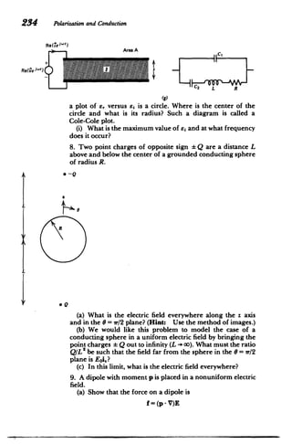
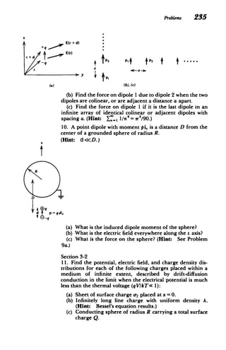
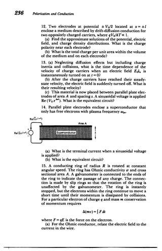
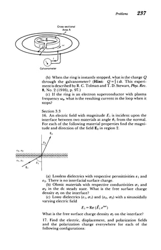
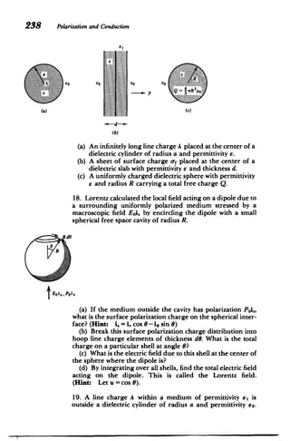
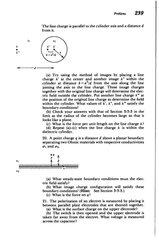
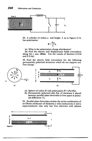
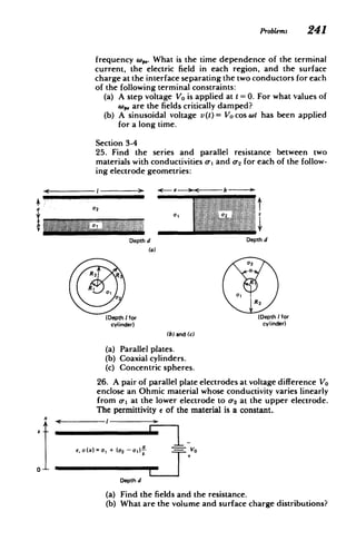
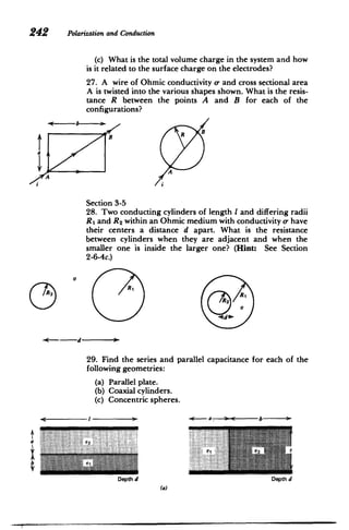
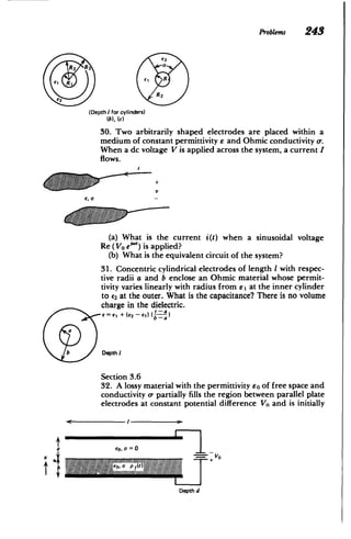
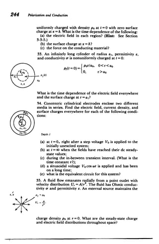
![Problems 245
+ VO
36. Charge maintained at constant density po at x =0 is car
ried away by a conducting fluid travelling at constant velocity
Ui. and is collected at x = 1.
6, U
U Cross-sectional
area A
P ~ P0
0
(a) What are the field and charge distributions within the
fluid if the electrodes are at potential difference VO?
(b) What is the force on the fluid?
(c) Repeat (a) and (b) if the voltage source is replaced by a
load resistor RL.
37. A dc voltage has been applied a long time to an open
circuited resistive-capacitive structure so that the voltage and
current have their steady-state distributions as given by (44).
Find the resulting discharging transients for voltage and
current if at t = 0 the terminals at z = 0 are suddenly:
(a) open circuited. Hint:
sinh a(z 1) sin
sI
(b) Short circuited. Hint:
=dz mir sinh al
I [a2
+ (mrr/L) 21
cosh a(z - .)
sin ((2n +1)7r
21
dz (2n + 1)-r cosh aL
2l[a2+ [(2n+1)7r 2
38. At t =0 a distributed resistive line as described in Section
3-6-4 has a step dc voltage Vo applied at z =0. The other end
at z = I is short circuited.
(a) What are the steady-state voltage and current dis
tributions?
(b) What is the time dependence of the voltage and current
during the transient interval? Hint:
sinh a(z -1) sin (5) dz = - mir sinh at
Ia2 + (mr/l)2]](https://image.slidesharecdn.com/mitres6002s08part1-211102045902/85/Mitres-6-002_s08_part1-273-320.jpg)
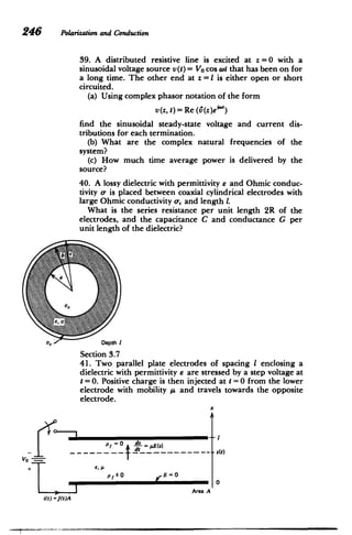
![Problems 247
(a) Using the charge conservation equation
3-2-1, show that the governing equation is
of Section
E aE
- + pE
-
at ax
J(t)
E
where J(t) is the current per unit electrode area through the
terminal wires. This current does not depend on x.
(b) By integrating (a) between the electrodes, relate the
current J(t) solely to the voltage and the electric field at the
two electrodes.
(c) For space charge limited conditions (E(x = 0) = 0), find
the time dependence of the electric field at the other elec
trode E(x = 1, t) before the charge front reaches it.
(Hint: With constant voltage, J(t) from (b) only depends on
E(x = 1, t). Using (a) at x = Iwith no charge, aE/8x = 0, we have
a single differential equation in E(x = 1, t).)
(d) What is the electric field acting on the charge front?
(Hint: There is no charge ahead of the front.)
(e) What is the position of the front s(t) as a function of
time?
(f) At what time does the front reach the other electrode?
(g) What are the steady-state distribution of potential,
electric field, and charge density? What is the steady-state
current density J(t -
>0)?
(h) Repeat (g) for nonspace charge limited conditions
when the emitter electric field E(x = 0) = EO is nonzero.
42. In a coaxial cylindrical geometry of length L, the inner
electrode at r = Ri is a source of positive ions with mobility /p
in the dielectric medium. The inner cylinder is at a dc voltage
Vo with respect to the outer cylinder.
E, (r = )= E
RO
R i _-=- O
Depth L
(a) The electric field at the emitter electrode is given as
Er(r= Rj) = Ej. If a current I flows, what are the steady-state
electric field and space charge distributions?
(b) What is the dc current I in terms of the voltage under
space charge limited conditions (Ei = 0)? Hint:
[r2 - RY2] 12
fdr
2_ 1/
= [r- Ri ]-
Ri
Ri Cos~-](https://image.slidesharecdn.com/mitres6002s08part1-211102045902/85/Mitres-6-002_s08_part1-275-320.jpg)
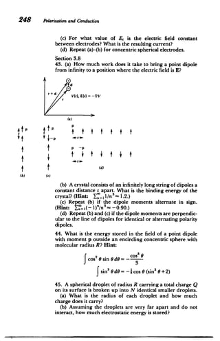
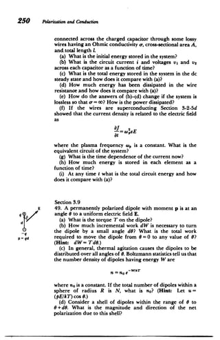
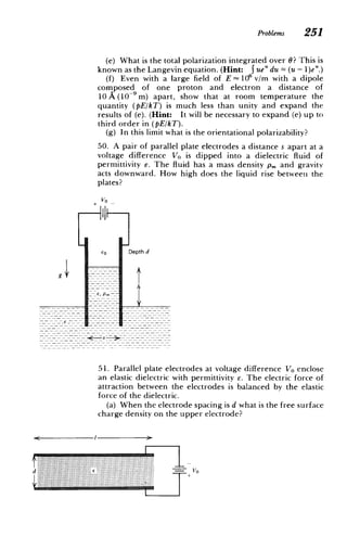
![252 Polarizationand Conduction
(b) What is the electric force per unit area that the elec
trode exerts on the dielectric interface?
(c) The elastic restoring force per unit area is given by the
relation
d
FA=Y in-
do
where Y is the modulus of elasticity and do is the unstressed
(Vo=0) thickness of the dielectric. Write a transcendental
expression for the equilibrium thickness of the dielectric.
(d) What is the minimum equilibrium dielectric thickness
and at what voltage does it occur? If a larger voltage is applied
there is no equilibrium and the dielectric fractures as the
electric stress overcomes the elastic restoring force. This is
called the theory of electromechanical breakdown. [See
K. H. Stark and C. G. Garton, Electric Strength of Irradiated
Polythene, Nature 176 (1955) 1225-26.]
52. An electret with permanent polarization Poi, and thick
ness d partially fills a free space capacitor. There is .nosurface
charge on the electret free space interface.
Area A
AA
seol
d V,
1- 1 11 PO+ V_
0
(a) What are the electric fields in each region?
(b) What is the force on the upper electrode?
53. A uniform distribution of free charge with density po is
between parallel plate electrodes at potential difference Vo.
Area A
(a) What is the energy stored in the system?
(b) Compare the capacitance to that when po =0.
(c) What is the total force on each electrode and on the
volume charge distribution?
(d) What is the total force on the system?
54. Coaxial cylindrical electrodes at voltage difference Vo are
partially filled with a polarized material. Find the force on this](https://image.slidesharecdn.com/mitres6002s08part1-211102045902/85/Mitres-6-002_s08_part1-280-320.jpg)
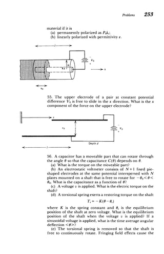
![254 Polarizationand Conduction
0 N rotor plates
I I
(N + 1) stator plates
2 C(0) C(O) = (CM + Cm n)
(6) = 2eoNR (00 --
)
s + (Cmax - Cmin)cos20
C(0) Cma.
Cnnin
0 0
-
0
0 b 0 it 2w
(e)
(b)
capacitance to vary smoothly between minimum and maxi
mum values of a dc value plus a single sinusoidal spatial term
C(6) = 1[C..+ Cmin] +1[Cm..- Cmin] cos 20
A sinusoidal voltage Vo cos wt is applied. What is the instan
taneous torque on the shaft?
(f) If the shaft is rotating at constant angular speed w. so
that
= w,.t + 8
where 8 is the angle of the shaft at t =0, under what condi
tions is the torque in (e) a constant? Hint:
I.
sin 26 coss ot = i sin 26(1 +cos 2awt)
= i sin'26 +- [sin (2(wt + ))-sin(2(wt - 6))]
(g) A time average torque To is required of the shaft. What
is the torque angle 8?
(h) What is the maximum torque that can be delivered?
This is called the pull-out torque. At what angle 8 does this
occur?
Section 3-10
57. The belt of a Van de Graaff generator has width w and
moves with speed U carrying a surface charge oy up to the
spherical dome of radius R.](https://image.slidesharecdn.com/mitres6002s08part1-211102045902/85/Mitres-6-002_s08_part1-282-320.jpg)
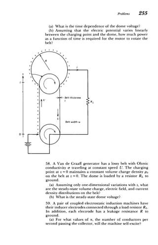
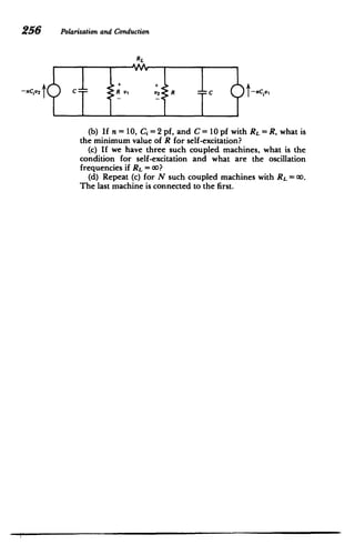

- The document discusses coordinate systems and vector relations for Cartesian, cylindrical, and spherical coordinate systems. It provides expressions for gradient, divergence, curl, and other vector operators in these coordinate systems. - It also lists Maxwell's equations in both integral and differential forms, as well as common constitutive relations and some physical constants. - The document presents a review of important vector concepts and their representations in different coordinate systems, as needed for electromagnetic field theory.


![[Deck] What's New in Spark-Iceberg Integration via DSV2.pptx](https://cdn.slidesharecdn.com/ss_thumbnails/deckwhatsnewinspark-icebergintegrationviadsv2-260210005337-25955b12-thumbnail.jpg?width=640&height=640&fit=bounds)

