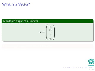
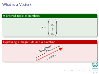
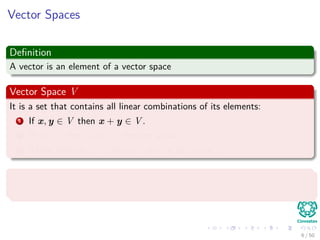
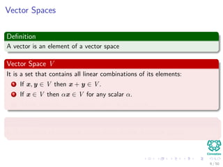
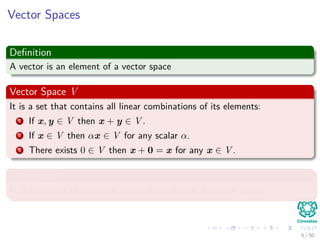
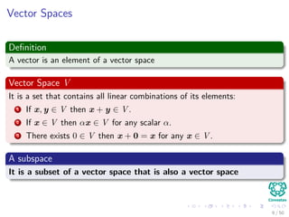
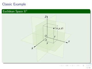
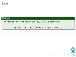
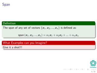
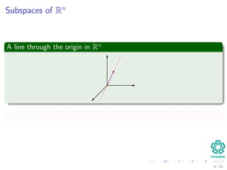
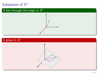
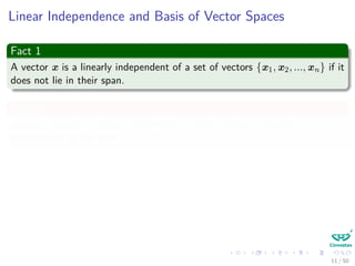
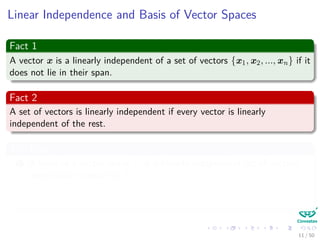
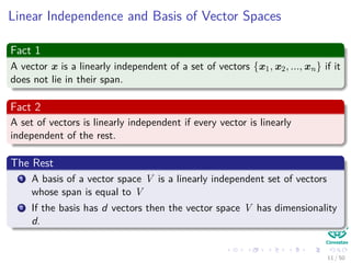
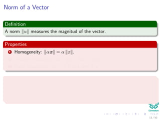
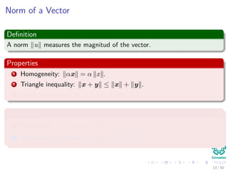
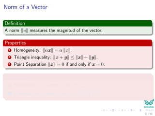
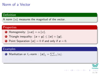
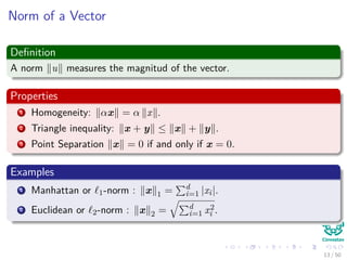
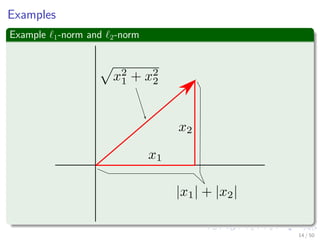
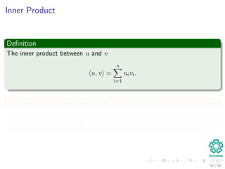
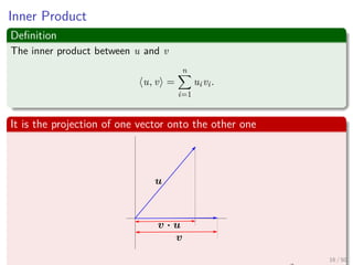
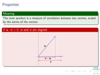
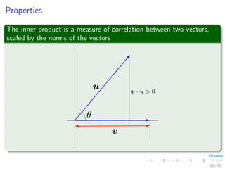
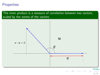
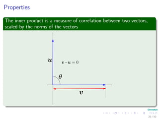
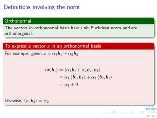
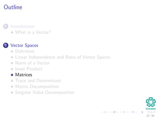
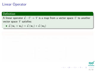
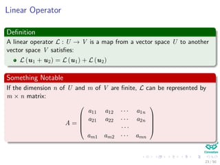
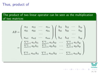
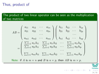
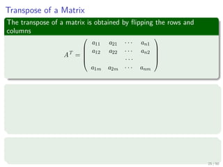
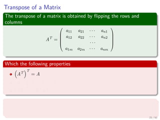
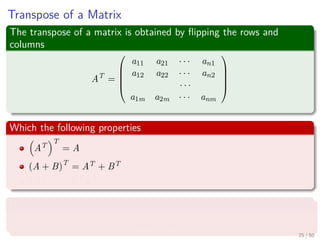
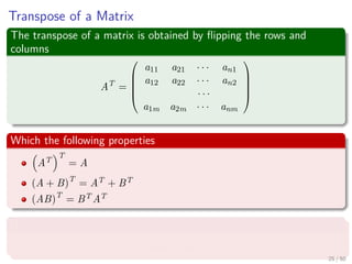
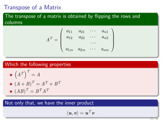
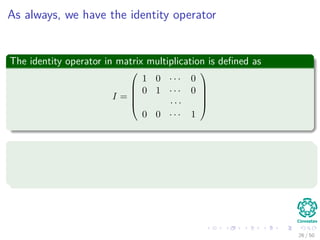
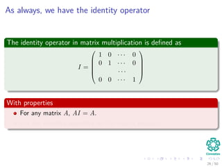
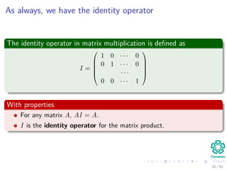
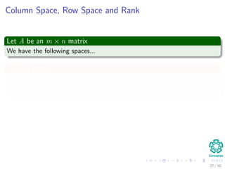
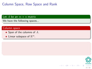
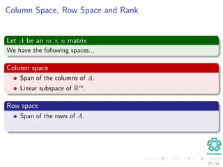
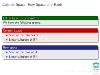
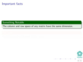
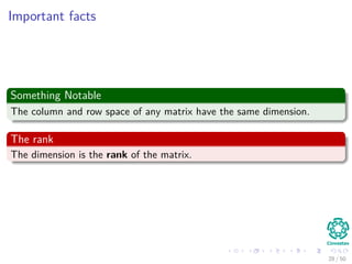
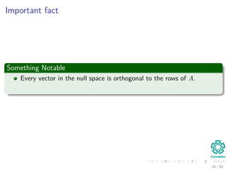
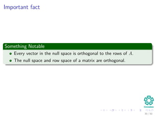
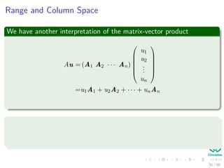
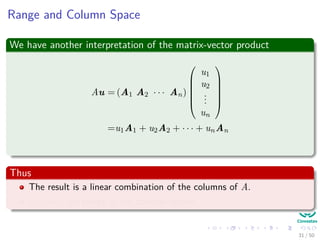
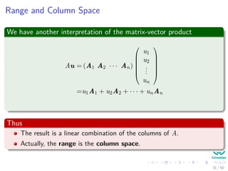
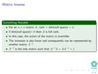
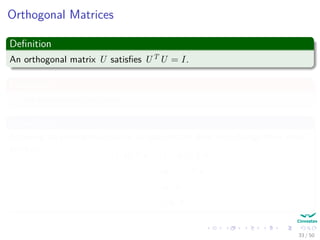
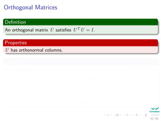
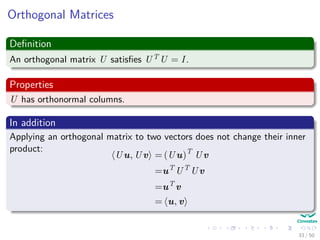
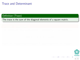
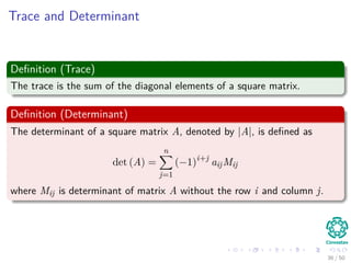
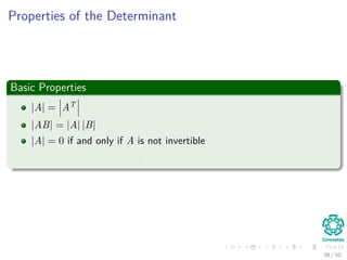
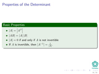
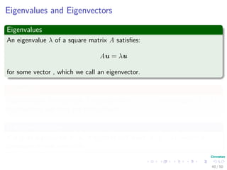
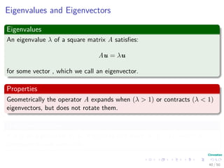
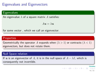
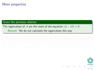
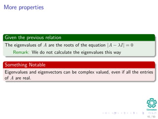
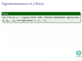
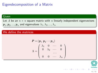
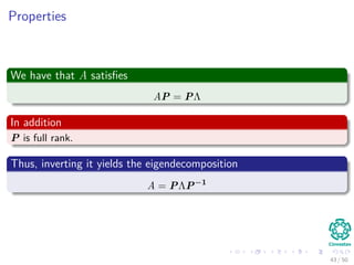
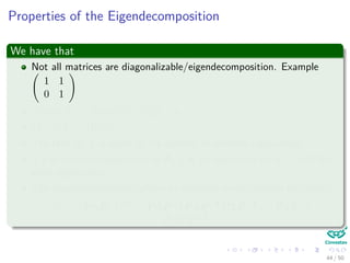
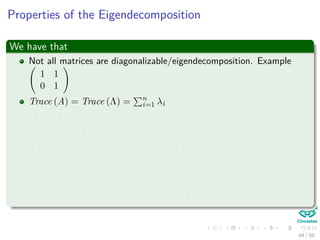
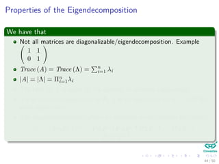
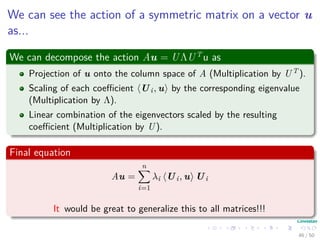
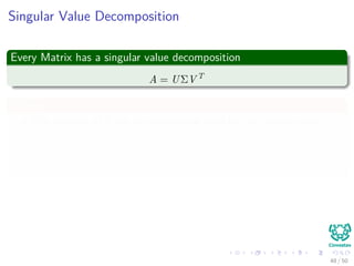
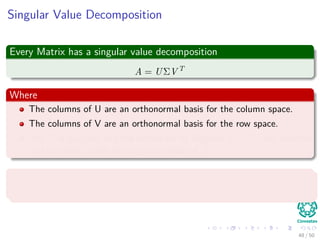
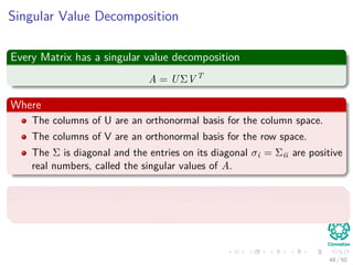
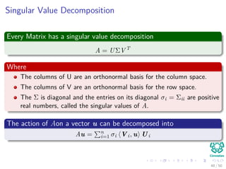
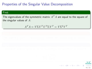
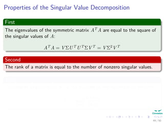
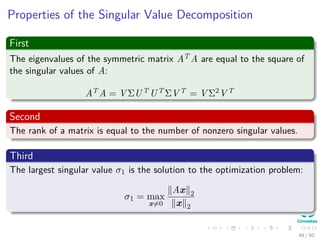
The document provides an introduction to linear algebra concepts for machine learning. It defines vectors as ordered tuples of numbers that express magnitude and direction. Vector spaces are sets that contain all linear combinations of vectors. Linear independence and basis of vector spaces are discussed. Norms measure the magnitude of a vector, with examples given of the 1-norm and 2-norm. Inner products measure the correlation between vectors. Matrices can represent linear operators between vector spaces. Key linear algebra concepts such as trace, determinant, and matrix decompositions are outlined for machine learning applications.

1. Machine Learning for Data Mining
Linear Algebra Review
Andres Mendez-Vazquez
May 14, 2015
1 / 50

2. Outline
1 Introduction
What is a Vector?
2 Vector Spaces
Definition
Linear Independence and Basis of Vector Spaces
Norm of a Vector
Inner Product
Matrices
Trace and Determinant
Matrix Decomposition
Singular Value Decomposition
2 / 50

3. Outline
1 Introduction
What is a Vector?
2 Vector Spaces
Definition
Linear Independence and Basis of Vector Spaces
Norm of a Vector
Inner Product
Matrices
Trace and Determinant
Matrix Decomposition
Singular Value Decomposition
3 / 50

4. What is a Vector?
A ordered tuple of numbers
x =






x1
x2
...
xn






Expressing a magnitude and a direction
4 / 50

5. What is a Vector?
A ordered tuple of numbers
x =






x1
x2
...
xn






Expressing a magnitude and a direction
Magnitude
Direction
4 / 50

6. Outline
1 Introduction
What is a Vector?
2 Vector Spaces
Definition
Linear Independence and Basis of Vector Spaces
Norm of a Vector
Inner Product
Matrices
Trace and Determinant
Matrix Decomposition
Singular Value Decomposition
5 / 50

7. Vector Spaces
Definition
A vector is an element of a vector space
Vector Space V
It is a set that contains all linear combinations of its elements:
1 If x, y ∈ V then x + y ∈ V .
2 If x ∈ V then αx ∈ V for any scalar α.
3 There exists 0 ∈ V then x + 0 = x for any x ∈ V .
A subspace
It is a subset of a vector space that is also a vector space
6 / 50

8. Vector Spaces
Definition
A vector is an element of a vector space
Vector Space V
It is a set that contains all linear combinations of its elements:
1 If x, y ∈ V then x + y ∈ V .
2 If x ∈ V then αx ∈ V for any scalar α.
3 There exists 0 ∈ V then x + 0 = x for any x ∈ V .
A subspace
It is a subset of a vector space that is also a vector space
6 / 50

9. Vector Spaces
Definition
A vector is an element of a vector space
Vector Space V
It is a set that contains all linear combinations of its elements:
1 If x, y ∈ V then x + y ∈ V .
2 If x ∈ V then αx ∈ V for any scalar α.
3 There exists 0 ∈ V then x + 0 = x for any x ∈ V .
A subspace
It is a subset of a vector space that is also a vector space
6 / 50

10. Vector Spaces
Definition
A vector is an element of a vector space
Vector Space V
It is a set that contains all linear combinations of its elements:
1 If x, y ∈ V then x + y ∈ V .
2 If x ∈ V then αx ∈ V for any scalar α.
3 There exists 0 ∈ V then x + 0 = x for any x ∈ V .
A subspace
It is a subset of a vector space that is also a vector space
6 / 50

11. Vector Spaces
Definition
A vector is an element of a vector space
Vector Space V
It is a set that contains all linear combinations of its elements:
1 If x, y ∈ V then x + y ∈ V .
2 If x ∈ V then αx ∈ V for any scalar α.
3 There exists 0 ∈ V then x + 0 = x for any x ∈ V .
A subspace
It is a subset of a vector space that is also a vector space
6 / 50

12. Classic Example
Euclidean Space R3
7 / 50

13. Span
Definition
The span of any set of vectors {x1, x2, ..., xn} is defined as:
span (x1, x2, ..., xn) = α1x1 + α2x2 + ... + αnxn
What Examples can you Imagine?
Give it a shot!!!
8 / 50

14. Span
Definition
The span of any set of vectors {x1, x2, ..., xn} is defined as:
span (x1, x2, ..., xn) = α1x1 + α2x2 + ... + αnxn
What Examples can you Imagine?
Give it a shot!!!
8 / 50

15. Subspaces of Rn
A line through the origin in Rn
A plane in Rn
9 / 50

16. Subspaces of Rn
A line through the origin in Rn
A plane in Rn
9 / 50

17. Outline
1 Introduction
What is a Vector?
2 Vector Spaces
Definition
Linear Independence and Basis of Vector Spaces
Norm of a Vector
Inner Product
Matrices
Trace and Determinant
Matrix Decomposition
Singular Value Decomposition
10 / 50

18. Linear Independence and Basis of Vector Spaces
Fact 1
A vector x is a linearly independent of a set of vectors {x1, x2, ..., xn} if it
does not lie in their span.
Fact 2
A set of vectors is linearly independent if every vector is linearly
independent of the rest.
The Rest
1 A basis of a vector space V is a linearly independent set of vectors
whose span is equal to V
2 If the basis has d vectors then the vector space V has dimensionality
d.
11 / 50

19. Linear Independence and Basis of Vector Spaces
Fact 1
A vector x is a linearly independent of a set of vectors {x1, x2, ..., xn} if it
does not lie in their span.
Fact 2
A set of vectors is linearly independent if every vector is linearly
independent of the rest.
The Rest
1 A basis of a vector space V is a linearly independent set of vectors
whose span is equal to V
2 If the basis has d vectors then the vector space V has dimensionality
d.
11 / 50

20. Linear Independence and Basis of Vector Spaces
Fact 1
A vector x is a linearly independent of a set of vectors {x1, x2, ..., xn} if it
does not lie in their span.
Fact 2
A set of vectors is linearly independent if every vector is linearly
independent of the rest.
The Rest
1 A basis of a vector space V is a linearly independent set of vectors
whose span is equal to V
2 If the basis has d vectors then the vector space V has dimensionality
d.
11 / 50

21. Outline
1 Introduction
What is a Vector?
2 Vector Spaces
Definition
Linear Independence and Basis of Vector Spaces
Norm of a Vector
Inner Product
Matrices
Trace and Determinant
Matrix Decomposition
Singular Value Decomposition
12 / 50

22. Norm of a Vector
Definition
A norm u measures the magnitud of the vector.
Properties
1 Homogeneity: αx = α x .
2 Triangle inequality: x + y ≤ x + y .
3 Point Separation x = 0 if and only if x = 0.
Examples
1 Manhattan or 1-norm : x 1 = d
i=1 |xi|.
2 Euclidean or 2-norm : x 2 = d
i=1 x2
i .
13 / 50

23. Norm of a Vector
Definition
A norm u measures the magnitud of the vector.
Properties
1 Homogeneity: αx = α x .
2 Triangle inequality: x + y ≤ x + y .
3 Point Separation x = 0 if and only if x = 0.
Examples
1 Manhattan or 1-norm : x 1 = d
i=1 |xi|.
2 Euclidean or 2-norm : x 2 = d
i=1 x2
i .
13 / 50

24. Norm of a Vector
Definition
A norm u measures the magnitud of the vector.
Properties
1 Homogeneity: αx = α x .
2 Triangle inequality: x + y ≤ x + y .
3 Point Separation x = 0 if and only if x = 0.
Examples
1 Manhattan or 1-norm : x 1 = d
i=1 |xi|.
2 Euclidean or 2-norm : x 2 = d
i=1 x2
i .
13 / 50

25. Norm of a Vector
Definition
A norm u measures the magnitud of the vector.
Properties
1 Homogeneity: αx = α x .
2 Triangle inequality: x + y ≤ x + y .
3 Point Separation x = 0 if and only if x = 0.
Examples
1 Manhattan or 1-norm : x 1 = d
i=1 |xi|.
2 Euclidean or 2-norm : x 2 = d
i=1 x2
i .
13 / 50

26. Norm of a Vector
Definition
A norm u measures the magnitud of the vector.
Properties
1 Homogeneity: αx = α x .
2 Triangle inequality: x + y ≤ x + y .
3 Point Separation x = 0 if and only if x = 0.
Examples
1 Manhattan or 1-norm : x 1 = d
i=1 |xi|.
2 Euclidean or 2-norm : x 2 = d
i=1 x2
i .
13 / 50

27. Norm of a Vector
Definition
A norm u measures the magnitud of the vector.
Properties
1 Homogeneity: αx = α x .
2 Triangle inequality: x + y ≤ x + y .
3 Point Separation x = 0 if and only if x = 0.
Examples
1 Manhattan or 1-norm : x 1 = d
i=1 |xi|.
2 Euclidean or 2-norm : x 2 = d
i=1 x2
i .
13 / 50

28. Examples
Example 1-norm and 2-norm
14 / 50

29. Outline
1 Introduction
What is a Vector?
2 Vector Spaces
Definition
Linear Independence and Basis of Vector Spaces
Norm of a Vector
Inner Product
Matrices
Trace and Determinant
Matrix Decomposition
Singular Value Decomposition
15 / 50

30. Inner Product
Definition
The inner product between u and v
u, v =
n
i=1
uivi.
It is the projection of one vector onto the other one
Remark: It is related to the Euclidean norm: u, u = u 2
2.
16 / 50

31. Inner Product
Definition
The inner product between u and v
u, v =
n
i=1
uivi.
It is the projection of one vector onto the other one
16 / 50

32. Properties
Meaning
The inner product is a measure of correlation between two vectors, scaled
by the norms of the vectors
if u · v > 0, u and v are aligned
17 / 50

33. Properties
Meaning
The inner product is a measure of correlation between two vectors, scaled
by the norms of the vectors
if u · v > 0, u and v are aligned
17 / 50

34. Properties
The inner product is a measure of correlation between two vectors,
scaled by the norms of the vectors
18 / 50

35. Properties
The inner product is a measure of correlation between two vectors,
scaled by the norms of the vectors
19 / 50

36. Properties
The inner product is a measure of correlation between two vectors,
scaled by the norms of the vectors
20 / 50

37. Definitions involving the norm
Orthonormal
The vectors in orthonormal basis have unit Euclidean norm and are
orthonorgonal.
To express a vector x in an orthonormal basis
For example, given x = α1b1 + α2b2
x, b1 = α1b1 + α2b2, b1
= α1 b1, b1 + α2 b2, b1
= α1 + 0
Likewise, x, b2 = α2
21 / 50

38. Definitions involving the norm
Orthonormal
The vectors in orthonormal basis have unit Euclidean norm and are
orthonorgonal.
To express a vector x in an orthonormal basis
For example, given x = α1b1 + α2b2
x, b1 = α1b1 + α2b2, b1
= α1 b1, b1 + α2 b2, b1
= α1 + 0
Likewise, x, b2 = α2
21 / 50

39. Definitions involving the norm
Orthonormal
The vectors in orthonormal basis have unit Euclidean norm and are
orthonorgonal.
To express a vector x in an orthonormal basis
For example, given x = α1b1 + α2b2
x, b1 = α1b1 + α2b2, b1
= α1 b1, b1 + α2 b2, b1
= α1 + 0
Likewise, x, b2 = α2
21 / 50

40. Outline
1 Introduction
What is a Vector?
2 Vector Spaces
Definition
Linear Independence and Basis of Vector Spaces
Norm of a Vector
Inner Product
Matrices
Trace and Determinant
Matrix Decomposition
Singular Value Decomposition
22 / 50

41. Linear Operator
Definition
A linear operator L : U → V is a map from a vector space U to another
vector space V satisfies:
L (u1 + u2) = L (u1) + L (u2)
Something Notable
If the dimension n of U and m of V are finite, L can be represented by
m × n matrix:
A =





a11 a12 · · · a1n
a21 a22 · · · a2n
· · ·
am1 am2 · · · amn





23 / 50

42. Linear Operator
Definition
A linear operator L : U → V is a map from a vector space U to another
vector space V satisfies:
L (u1 + u2) = L (u1) + L (u2)
Something Notable
If the dimension n of U and m of V are finite, L can be represented by
m × n matrix:
A =





a11 a12 · · · a1n
a21 a22 · · · a2n
· · ·
am1 am2 · · · amn





23 / 50

43. Thus, product of
The product of two linear operator can be seen as the multiplication
of two matrices
AB =





a11 a12 · · · a1n
a21 a22 · · · a2n
· · ·
am1 am2 · · · amn










b11 b12 · · · b1p
b21 b22 · · · b2p
· · ·
bn1 bn2 · · · bnp





=





n
i=1 a1ibi1
n
i=1 a1ibi2 · · · n
i=1 a1ibip
n
i=1 a2ibi1
n
i=1 a2ibi2 · · · n
i=1 a2ibip
· · ·
n
i=1 amibi1
n
i=1 amibi2 · · · n
i=1 amibip





Note: if A is m × n and B is n × p, then AB is m × p.
24 / 50

44. Thus, product of
The product of two linear operator can be seen as the multiplication
of two matrices
AB =





a11 a12 · · · a1n
a21 a22 · · · a2n
· · ·
am1 am2 · · · amn










b11 b12 · · · b1p
b21 b22 · · · b2p
· · ·
bn1 bn2 · · · bnp





=





n
i=1 a1ibi1
n
i=1 a1ibi2 · · · n
i=1 a1ibip
n
i=1 a2ibi1
n
i=1 a2ibi2 · · · n
i=1 a2ibip
· · ·
n
i=1 amibi1
n
i=1 amibi2 · · · n
i=1 amibip





Note: if A is m × n and B is n × p, then AB is m × p.
24 / 50

45. Transpose of a Matrix
The transpose of a matrix is obtained by flipping the rows and
columns
AT
=





a11 a21 · · · an1
a12 a22 · · · an2
· · ·
a1m a2m · · · anm





Which the following properties
AT
T
= A
(A + B)T
= AT + BT
(AB)T
= BT AT
Not only that, we have the inner product
u, v = uT
v
25 / 50

46. Transpose of a Matrix
The transpose of a matrix is obtained by flipping the rows and
columns
AT
=





a11 a21 · · · an1
a12 a22 · · · an2
· · ·
a1m a2m · · · anm





Which the following properties
AT
T
= A
(A + B)T
= AT + BT
(AB)T
= BT AT
Not only that, we have the inner product
u, v = uT
v
25 / 50

47. Transpose of a Matrix
The transpose of a matrix is obtained by flipping the rows and
columns
AT
=





a11 a21 · · · an1
a12 a22 · · · an2
· · ·
a1m a2m · · · anm





Which the following properties
AT
T
= A
(A + B)T
= AT + BT
(AB)T
= BT AT
Not only that, we have the inner product
u, v = uT
v
25 / 50

48. Transpose of a Matrix
The transpose of a matrix is obtained by flipping the rows and
columns
AT
=





a11 a21 · · · an1
a12 a22 · · · an2
· · ·
a1m a2m · · · anm





Which the following properties
AT
T
= A
(A + B)T
= AT + BT
(AB)T
= BT AT
Not only that, we have the inner product
u, v = uT
v
25 / 50

49. Transpose of a Matrix
The transpose of a matrix is obtained by flipping the rows and
columns
AT
=





a11 a21 · · · an1
a12 a22 · · · an2
· · ·
a1m a2m · · · anm





Which the following properties
AT
T
= A
(A + B)T
= AT + BT
(AB)T
= BT AT
Not only that, we have the inner product
u, v = uT
v
25 / 50

50. As always, we have the identity operator
The identity operator in matrix multiplication is defined as
I =





1 0 · · · 0
0 1 · · · 0
· · ·
0 0 · · · 1





With properties
For any matrix A, AI = A.
I is the identity operator for the matrix product.
26 / 50

51. As always, we have the identity operator
The identity operator in matrix multiplication is defined as
I =





1 0 · · · 0
0 1 · · · 0
· · ·
0 0 · · · 1





With properties
For any matrix A, AI = A.
I is the identity operator for the matrix product.
26 / 50

52. As always, we have the identity operator
The identity operator in matrix multiplication is defined as
I =





1 0 · · · 0
0 1 · · · 0
· · ·
0 0 · · · 1





With properties
For any matrix A, AI = A.
I is the identity operator for the matrix product.
26 / 50

53. Column Space, Row Space and Rank
Let A be an m × n matrix
We have the following spaces...
Column space
Span of the columns of A.
Linear subspace of Rm.
Row space
Span of the rows of A.
Linear subspace of Rn.
27 / 50

54. Column Space, Row Space and Rank
Let A be an m × n matrix
We have the following spaces...
Column space
Span of the columns of A.
Linear subspace of Rm.
Row space
Span of the rows of A.
Linear subspace of Rn.
27 / 50

55. Column Space, Row Space and Rank
Let A be an m × n matrix
We have the following spaces...
Column space
Span of the columns of A.
Linear subspace of Rm.
Row space
Span of the rows of A.
Linear subspace of Rn.
27 / 50

56. Column Space, Row Space and Rank
Let A be an m × n matrix
We have the following spaces...
Column space
Span of the columns of A.
Linear subspace of Rm.
Row space
Span of the rows of A.
Linear subspace of Rn.
27 / 50

57. Important facts
Something Notable
The column and row space of any matrix have the same dimension.
The rank
The dimension is the rank of the matrix.
28 / 50

58. Important facts
Something Notable
The column and row space of any matrix have the same dimension.
The rank
The dimension is the rank of the matrix.
28 / 50

59. Range and Null Space
Range
Set of vectors equal to Au for some u ∈ Rn.
Range (A) = {x|x = Au for some u ∈ Rn
}
It is a linear subspace of Rm and also called the column space of A.
Null Space
We have the following definition
Null Space (A) = {u|Au = 0}
It is a linear subspace of Rm.
29 / 50

60. Range and Null Space
Range
Set of vectors equal to Au for some u ∈ Rn.
Range (A) = {x|x = Au for some u ∈ Rn
}
It is a linear subspace of Rm and also called the column space of A.
Null Space
We have the following definition
Null Space (A) = {u|Au = 0}
It is a linear subspace of Rm.
29 / 50

61. Range and Null Space
Range
Set of vectors equal to Au for some u ∈ Rn.
Range (A) = {x|x = Au for some u ∈ Rn
}
It is a linear subspace of Rm and also called the column space of A.
Null Space
We have the following definition
Null Space (A) = {u|Au = 0}
It is a linear subspace of Rm.
29 / 50

62. Range and Null Space
Range
Set of vectors equal to Au for some u ∈ Rn.
Range (A) = {x|x = Au for some u ∈ Rn
}
It is a linear subspace of Rm and also called the column space of A.
Null Space
We have the following definition
Null Space (A) = {u|Au = 0}
It is a linear subspace of Rm.
29 / 50

63. Important fact
Something Notable
Every vector in the null space is orthogonal to the rows of A.
The null space and row space of a matrix are orthogonal.
30 / 50

64. Important fact
Something Notable
Every vector in the null space is orthogonal to the rows of A.
The null space and row space of a matrix are orthogonal.
30 / 50

65. Range and Column Space
We have another interpretation of the matrix-vector product
Au = (A1 A2 · · · An)






u1
u2
...
un






=u1A1 + u2A2 + · · · + unAn
Thus
The result is a linear combination of the columns of A.
Actually, the range is the column space.
31 / 50

66. Range and Column Space
We have another interpretation of the matrix-vector product
Au = (A1 A2 · · · An)






u1
u2
...
un






=u1A1 + u2A2 + · · · + unAn
Thus
The result is a linear combination of the columns of A.
Actually, the range is the column space.
31 / 50

67. Range and Column Space
We have another interpretation of the matrix-vector product
Au = (A1 A2 · · · An)






u1
u2
...
un






=u1A1 + u2A2 + · · · + unAn
Thus
The result is a linear combination of the columns of A.
Actually, the range is the column space.
31 / 50

68. Matrix Inverse
Something Notable
For an n × n matrix A: rank + dim(null space) = n.
if dim(null space)= 0 then A is full rank.
In this case, the action of the matrix is invertible.
The inversion is also linear and consequently can be represented by
another matrix A−1.
A−1 is the only matrix such that A−1A = AA−1 = I.
32 / 50

69. Matrix Inverse
Something Notable
For an n × n matrix A: rank + dim(null space) = n.
if dim(null space)= 0 then A is full rank.
In this case, the action of the matrix is invertible.
The inversion is also linear and consequently can be represented by
another matrix A−1.
A−1 is the only matrix such that A−1A = AA−1 = I.
32 / 50

70. Matrix Inverse
Something Notable
For an n × n matrix A: rank + dim(null space) = n.
if dim(null space)= 0 then A is full rank.
In this case, the action of the matrix is invertible.
The inversion is also linear and consequently can be represented by
another matrix A−1.
A−1 is the only matrix such that A−1A = AA−1 = I.
32 / 50

71. Matrix Inverse
Something Notable
For an n × n matrix A: rank + dim(null space) = n.
if dim(null space)= 0 then A is full rank.
In this case, the action of the matrix is invertible.
The inversion is also linear and consequently can be represented by
another matrix A−1.
A−1 is the only matrix such that A−1A = AA−1 = I.
32 / 50

72. Matrix Inverse
Something Notable
For an n × n matrix A: rank + dim(null space) = n.
if dim(null space)= 0 then A is full rank.
In this case, the action of the matrix is invertible.
The inversion is also linear and consequently can be represented by
another matrix A−1.
A−1 is the only matrix such that A−1A = AA−1 = I.
32 / 50

73. Orthogonal Matrices
Definition
An orthogonal matrix U satisfies UT U = I.
Properties
U has orthonormal columns.
In addition
Applying an orthogonal matrix to two vectors does not change their inner
product:
Uu, Uv = (Uu)T
Uv
=uT
UT
Uv
=uT
v
= u, v
33 / 50

74. Orthogonal Matrices
Definition
An orthogonal matrix U satisfies UT U = I.
Properties
U has orthonormal columns.
In addition
Applying an orthogonal matrix to two vectors does not change their inner
product:
Uu, Uv = (Uu)T
Uv
=uT
UT
Uv
=uT
v
= u, v
33 / 50

75. Orthogonal Matrices
Definition
An orthogonal matrix U satisfies UT U = I.
Properties
U has orthonormal columns.
In addition
Applying an orthogonal matrix to two vectors does not change their inner
product:
Uu, Uv = (Uu)T
Uv
=uT
UT
Uv
=uT
v
= u, v
33 / 50

76. Example
A classic one
Matrices representing rotations are orthogonal.
34 / 50

77. Outline
1 Introduction
What is a Vector?
2 Vector Spaces
Definition
Linear Independence and Basis of Vector Spaces
Norm of a Vector
Inner Product
Matrices
Trace and Determinant
Matrix Decomposition
Singular Value Decomposition
35 / 50

78. Trace and Determinant
Definition (Trace)
The trace is the sum of the diagonal elements of a square matrix.
Definition (Determinant)
The determinant of a square matrix A, denoted by |A|, is defined as
det (A) =
n
j=1
(−1)i+j
aijMij
where Mij is determinant of matrix A without the row i and column j.
36 / 50

79. Trace and Determinant
Definition (Trace)
The trace is the sum of the diagonal elements of a square matrix.
Definition (Determinant)
The determinant of a square matrix A, denoted by |A|, is defined as
det (A) =
n
j=1
(−1)i+j
aijMij
where Mij is determinant of matrix A without the row i and column j.
36 / 50

80. Special Case
For a 2 × 2 matrix A =
a b
c d
|A| = ad − bc
The absolute value of |A|is the area of the parallelogram given by the
rows of A
37 / 50

81. Special Case
For a 2 × 2 matrix A =
a b
c d
|A| = ad − bc
The absolute value of |A|is the area of the parallelogram given by the
rows of A
37 / 50

82. Properties of the Determinant
Basic Properties
|A| = AT
|AB| = |A| |B|
|A| = 0 if and only if A is not invertible
If A is invertible, then A−1 = 1
|A| .
38 / 50

83. Properties of the Determinant
Basic Properties
|A| = AT
|AB| = |A| |B|
|A| = 0 if and only if A is not invertible
If A is invertible, then A−1 = 1
|A| .
38 / 50

84. Properties of the Determinant
Basic Properties
|A| = AT
|AB| = |A| |B|
|A| = 0 if and only if A is not invertible
If A is invertible, then A−1 = 1
|A| .
38 / 50

85. Properties of the Determinant
Basic Properties
|A| = AT
|AB| = |A| |B|
|A| = 0 if and only if A is not invertible
If A is invertible, then A−1 = 1
|A| .
38 / 50

86. Outline
1 Introduction
What is a Vector?
2 Vector Spaces
Definition
Linear Independence and Basis of Vector Spaces
Norm of a Vector
Inner Product
Matrices
Trace and Determinant
Matrix Decomposition
Singular Value Decomposition
39 / 50

87. Eigenvalues and Eigenvectors
Eigenvalues
An eigenvalue λ of a square matrix A satisfies:
Au = λu
for some vector , which we call an eigenvector.
Properties
Geometrically the operator A expands when (λ > 1) or contracts (λ < 1)
eigenvectors, but does not rotate them.
Null Space relation
If u is an eigenvector of A, it is in the null space of A − λI, which is
consequently not invertible.
40 / 50

88. Eigenvalues and Eigenvectors
Eigenvalues
An eigenvalue λ of a square matrix A satisfies:
Au = λu
for some vector , which we call an eigenvector.
Properties
Geometrically the operator A expands when (λ > 1) or contracts (λ < 1)
eigenvectors, but does not rotate them.
Null Space relation
If u is an eigenvector of A, it is in the null space of A − λI, which is
consequently not invertible.
40 / 50

89. Eigenvalues and Eigenvectors
Eigenvalues
An eigenvalue λ of a square matrix A satisfies:
Au = λu
for some vector , which we call an eigenvector.
Properties
Geometrically the operator A expands when (λ > 1) or contracts (λ < 1)
eigenvectors, but does not rotate them.
Null Space relation
If u is an eigenvector of A, it is in the null space of A − λI, which is
consequently not invertible.
40 / 50

90. More properties
Given the previous relation
The eigenvalues of A are the roots of the equation |A − λI| = 0
Remark: We do not calculate the eigenvalues this way
Something Notable
Eigenvalues and eigenvectors can be complex valued, even if all the entries
of A are real.
41 / 50

91. More properties
Given the previous relation
The eigenvalues of A are the roots of the equation |A − λI| = 0
Remark: We do not calculate the eigenvalues this way
Something Notable
Eigenvalues and eigenvectors can be complex valued, even if all the entries
of A are real.
41 / 50

92. Eigendecomposition of a Matrix
Given
Let A be an n × n square matrix with n linearly independent eigenvectors
p1, p2, ..., pn and eigenvalues λ1, λ2, ..., λn
We define the matrices
P = (p1 p2 · · · pn)
Λ =





λ1 0 · · · 0
0 λ2 · · · 0
· · ·
0 0 · · · λn





42 / 50

93. Eigendecomposition of a Matrix
Given
Let A be an n × n square matrix with n linearly independent eigenvectors
p1, p2, ..., pn and eigenvalues λ1, λ2, ..., λn
We define the matrices
P = (p1 p2 · · · pn)
Λ =





λ1 0 · · · 0
0 λ2 · · · 0
· · ·
0 0 · · · λn





42 / 50

94. Properties
We have that A satisfies
AP = PΛ
In addition
P is full rank.
Thus, inverting it yields the eigendecomposition
A = PΛP−1
43 / 50

95. Properties
We have that A satisfies
AP = PΛ
In addition
P is full rank.
Thus, inverting it yields the eigendecomposition
A = PΛP−1
43 / 50

96. Properties
We have that A satisfies
AP = PΛ
In addition
P is full rank.
Thus, inverting it yields the eigendecomposition
A = PΛP−1
43 / 50

97. Properties of the Eigendecomposition
We have that
Not all matrices are diagonalizable/eigendecomposition. Example
1 1
0 1
Trace (A) = Trace (Λ) = n
i=1 λi
|A| = |Λ| = Πn
i=1λi
The rank of A is equal to the number of nonzero eigenvalues.
If λ is anonzero eigenvalue of A, 1
λ is an eigenvalue of A−1 with the
same eigenvector.
The eigendecompositon allows to compute matrix powers efficiently:
Am = PΛP−1 m
= PΛP−1PΛP−1PΛP−1 . . . PΛP−1 =
PΛmP−1
44 / 50

98. Properties of the Eigendecomposition
We have that
Not all matrices are diagonalizable/eigendecomposition. Example
1 1
0 1
Trace (A) = Trace (Λ) = n
i=1 λi
|A| = |Λ| = Πn
i=1λi
The rank of A is equal to the number of nonzero eigenvalues.
If λ is anonzero eigenvalue of A, 1
λ is an eigenvalue of A−1 with the
same eigenvector.
The eigendecompositon allows to compute matrix powers efficiently:
Am = PΛP−1 m
= PΛP−1PΛP−1PΛP−1 . . . PΛP−1 =
PΛmP−1
44 / 50

99. Properties of the Eigendecomposition
We have that
Not all matrices are diagonalizable/eigendecomposition. Example
1 1
0 1
Trace (A) = Trace (Λ) = n
i=1 λi
|A| = |Λ| = Πn
i=1λi
The rank of A is equal to the number of nonzero eigenvalues.
If λ is anonzero eigenvalue of A, 1
λ is an eigenvalue of A−1 with the
same eigenvector.
The eigendecompositon allows to compute matrix powers efficiently:
Am = PΛP−1 m
= PΛP−1PΛP−1PΛP−1 . . . PΛP−1 =
PΛmP−1
44 / 50

100. Properties of the Eigendecomposition
We have that
Not all matrices are diagonalizable/eigendecomposition. Example
1 1
0 1
Trace (A) = Trace (Λ) = n
i=1 λi
|A| = |Λ| = Πn
i=1λi
The rank of A is equal to the number of nonzero eigenvalues.
If λ is anonzero eigenvalue of A, 1
λ is an eigenvalue of A−1 with the
same eigenvector.
The eigendecompositon allows to compute matrix powers efficiently:
Am = PΛP−1 m
= PΛP−1PΛP−1PΛP−1 . . . PΛP−1 =
PΛmP−1
44 / 50

101. Properties of the Eigendecomposition
We have that
Not all matrices are diagonalizable/eigendecomposition. Example
1 1
0 1
Trace (A) = Trace (Λ) = n
i=1 λi
|A| = |Λ| = Πn
i=1λi
The rank of A is equal to the number of nonzero eigenvalues.
If λ is anonzero eigenvalue of A, 1
λ is an eigenvalue of A−1 with the
same eigenvector.
The eigendecompositon allows to compute matrix powers efficiently:
Am = PΛP−1 m
= PΛP−1PΛP−1PΛP−1 . . . PΛP−1 =
PΛmP−1
44 / 50

102. Properties of the Eigendecomposition
We have that
Not all matrices are diagonalizable/eigendecomposition. Example
1 1
0 1
Trace (A) = Trace (Λ) = n
i=1 λi
|A| = |Λ| = Πn
i=1λi
The rank of A is equal to the number of nonzero eigenvalues.
If λ is anonzero eigenvalue of A, 1
λ is an eigenvalue of A−1 with the
same eigenvector.
The eigendecompositon allows to compute matrix powers efficiently:
Am = PΛP−1 m
= PΛP−1PΛP−1PΛP−1 . . . PΛP−1 =
PΛmP−1
44 / 50

103. Eigendecomposition of a Symmetric Matrix
When A symmetric, we have
If A = AT then A is symmetric.
The eigenvalues of symmetric matrices are real.
The eigenvectors of symmetric matrices are orthonormal.
Consequently, the eigendecomposition becomes A = UΛUT for Λ
real and U orthogonal.
The eigenvectors of A are an orthonormal basis for the column space
and row space.
45 / 50

104. Eigendecomposition of a Symmetric Matrix
When A symmetric, we have
If A = AT then A is symmetric.
The eigenvalues of symmetric matrices are real.
The eigenvectors of symmetric matrices are orthonormal.
Consequently, the eigendecomposition becomes A = UΛUT for Λ
real and U orthogonal.
The eigenvectors of A are an orthonormal basis for the column space
and row space.
45 / 50

105. Eigendecomposition of a Symmetric Matrix
When A symmetric, we have
If A = AT then A is symmetric.
The eigenvalues of symmetric matrices are real.
The eigenvectors of symmetric matrices are orthonormal.
Consequently, the eigendecomposition becomes A = UΛUT for Λ
real and U orthogonal.
The eigenvectors of A are an orthonormal basis for the column space
and row space.
45 / 50

106. Eigendecomposition of a Symmetric Matrix
When A symmetric, we have
If A = AT then A is symmetric.
The eigenvalues of symmetric matrices are real.
The eigenvectors of symmetric matrices are orthonormal.
Consequently, the eigendecomposition becomes A = UΛUT for Λ
real and U orthogonal.
The eigenvectors of A are an orthonormal basis for the column space
and row space.
45 / 50

107. Eigendecomposition of a Symmetric Matrix
When A symmetric, we have
If A = AT then A is symmetric.
The eigenvalues of symmetric matrices are real.
The eigenvectors of symmetric matrices are orthonormal.
Consequently, the eigendecomposition becomes A = UΛUT for Λ
real and U orthogonal.
The eigenvectors of A are an orthonormal basis for the column space
and row space.
45 / 50

108. We can see the action of a symmetric matrix on a vector u
as...
We can decompose the action Au = UΛUT
u as
Projection of u onto the column space of A (Multiplication by UT ).
Scaling of each coefficient Ui, u by the corresponding eigenvalue
(Multiplication by Λ).
Linear combination of the eigenvectors scaled by the resulting
coefficient (Multiplication by U).
Final equation
Au =
n
i=1
λi Ui, u Ui
It would be great to generalize this to all matrices!!!
46 / 50

109. We can see the action of a symmetric matrix on a vector u
as...
We can decompose the action Au = UΛUT
u as
Projection of u onto the column space of A (Multiplication by UT ).
Scaling of each coefficient Ui, u by the corresponding eigenvalue
(Multiplication by Λ).
Linear combination of the eigenvectors scaled by the resulting
coefficient (Multiplication by U).
Final equation
Au =
n
i=1
λi Ui, u Ui
It would be great to generalize this to all matrices!!!
46 / 50

110. We can see the action of a symmetric matrix on a vector u
as...
We can decompose the action Au = UΛUT
u as
Projection of u onto the column space of A (Multiplication by UT ).
Scaling of each coefficient Ui, u by the corresponding eigenvalue
(Multiplication by Λ).
Linear combination of the eigenvectors scaled by the resulting
coefficient (Multiplication by U).
Final equation
Au =
n
i=1
λi Ui, u Ui
It would be great to generalize this to all matrices!!!
46 / 50

111. We can see the action of a symmetric matrix on a vector u
as...
We can decompose the action Au = UΛUT
u as
Projection of u onto the column space of A (Multiplication by UT ).
Scaling of each coefficient Ui, u by the corresponding eigenvalue
(Multiplication by Λ).
Linear combination of the eigenvectors scaled by the resulting
coefficient (Multiplication by U).
Final equation
Au =
n
i=1
λi Ui, u Ui
It would be great to generalize this to all matrices!!!
46 / 50

112. We can see the action of a symmetric matrix on a vector u
as...
We can decompose the action Au = UΛUT
u as
Projection of u onto the column space of A (Multiplication by UT ).
Scaling of each coefficient Ui, u by the corresponding eigenvalue
(Multiplication by Λ).
Linear combination of the eigenvectors scaled by the resulting
coefficient (Multiplication by U).
Final equation
Au =
n
i=1
λi Ui, u Ui
It would be great to generalize this to all matrices!!!
46 / 50

113. Outline
1 Introduction
What is a Vector?
2 Vector Spaces
Definition
Linear Independence and Basis of Vector Spaces
Norm of a Vector
Inner Product
Matrices
Trace and Determinant
Matrix Decomposition
Singular Value Decomposition
47 / 50

114. Singular Value Decomposition
Every Matrix has a singular value decomposition
A = UΣV T
Where
The columns of U are an orthonormal basis for the column space.
The columns of V are an orthonormal basis for the row space.
The Σ is diagonal and the entries on its diagonal σi = Σii are positive
real numbers, called the singular values of A.
The action of Aon a vector u can be decomposed into
Au = n
i=1 σi Vi, u Ui
48 / 50

115. Singular Value Decomposition
Every Matrix has a singular value decomposition
A = UΣV T
Where
The columns of U are an orthonormal basis for the column space.
The columns of V are an orthonormal basis for the row space.
The Σ is diagonal and the entries on its diagonal σi = Σii are positive
real numbers, called the singular values of A.
The action of Aon a vector u can be decomposed into
Au = n
i=1 σi Vi, u Ui
48 / 50

116. Singular Value Decomposition
Every Matrix has a singular value decomposition
A = UΣV T
Where
The columns of U are an orthonormal basis for the column space.
The columns of V are an orthonormal basis for the row space.
The Σ is diagonal and the entries on its diagonal σi = Σii are positive
real numbers, called the singular values of A.
The action of Aon a vector u can be decomposed into
Au = n
i=1 σi Vi, u Ui
48 / 50

117. Singular Value Decomposition
Every Matrix has a singular value decomposition
A = UΣV T
Where
The columns of U are an orthonormal basis for the column space.
The columns of V are an orthonormal basis for the row space.
The Σ is diagonal and the entries on its diagonal σi = Σii are positive
real numbers, called the singular values of A.
The action of Aon a vector u can be decomposed into
Au = n
i=1 σi Vi, u Ui
48 / 50

118. Properties of the Singular Value Decomposition
First
The eigenvalues of the symmetric matrix AT A are equal to the square of
the singular values of A:
AT A = V ΣUT UT ΣV T = V Σ2V T
Second
The rank of a matrix is equal to the number of nonzero singular values.
Third
The largest singular value σ1 is the solution to the optimization problem:
σ1 = max
x=0
Ax 2
x 2
49 / 50

119. Properties of the Singular Value Decomposition
First
The eigenvalues of the symmetric matrix AT A are equal to the square of
the singular values of A:
AT A = V ΣUT UT ΣV T = V Σ2V T
Second
The rank of a matrix is equal to the number of nonzero singular values.
Third
The largest singular value σ1 is the solution to the optimization problem:
σ1 = max
x=0
Ax 2
x 2
49 / 50

120. Properties of the Singular Value Decomposition
First
The eigenvalues of the symmetric matrix AT A are equal to the square of
the singular values of A:
AT A = V ΣUT UT ΣV T = V Σ2V T
Second
The rank of a matrix is equal to the number of nonzero singular values.
Third
The largest singular value σ1 is the solution to the optimization problem:
σ1 = max
x=0
Ax 2
x 2
49 / 50

121. Properties of the Singular Value Decomposition
Remark
It can be verified that the largest singular value satisfies the properties of a
norm, it is called the spectral norm of the matrix.
Finally
In statistics analyzing data with the singular value decomposition is called
Principal Component Analysis.
50 / 50

122. Properties of the Singular Value Decomposition
Remark
It can be verified that the largest singular value satisfies the properties of a
norm, it is called the spectral norm of the matrix.
Finally
In statistics analyzing data with the singular value decomposition is called
Principal Component Analysis.
50 / 50