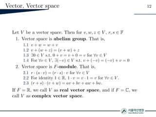
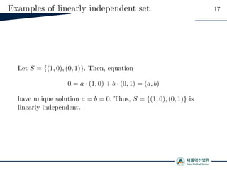
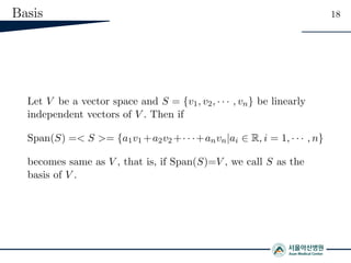
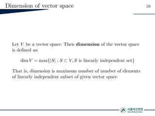
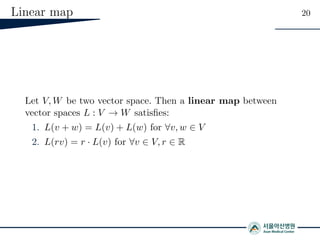
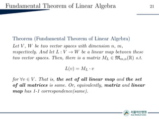
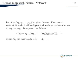
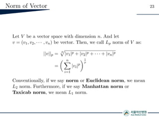
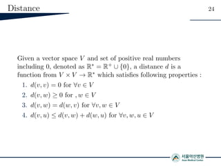
The document provides a comprehensive overview of mathematical concepts essential for deep learning, including linear algebra, manifolds, and the universal approximation theorem. It discusses various elements of vector spaces, linear maps, and their applications in neural networks. Additionally, it addresses the manifold hypothesis and conjecture, emphasizing their significance in understanding high-dimensional data structures.

1. Mathematics for Deep Learning
Ryoungwoo Jang, M.D.
University of Ulsan, Asan Medical Center

2. This pdf file is compiled in LATEX.
Every picture was drawn by Python.

3. Outline 3
Recommendation
Introduction
Linear Algebra
Manifold
Universal Approximation Theorem

4. Recommendation

5. Recommendation 5
Easy to start, easy to finish :
Calculus : James Stewart, Calculus
Linear algebra : Gilbert Strang, Introduction to Linear
Algebra
Mathematical Statistics : Hogg, Introduction to
Mathematical Statistics
Warning! - easy to start, hard to finish :
Calculus : 김홍종, 미적분학
Linear Algebra : 이인석 - 선형대수와 군
Mathematical Statistics : 김우철 - 수리통계학

6. Introduction

7. Introduction 7
Today’s Goal :
Linear Algebra, Manifold, Manifold Hypothesis,
Manifold Conjecture, Universal Approximation Theorem

8. Linear Algebra

9. Vector, Vector space 9
In high school, vector was
something that has size and direction

10. Vector, Vector space 10
In modern mathematics, · · ·

11. Vector, Vector space 11
Vector is element of Vector space.
Then, what is vector space?

12. Vector, Vector space 12
Let V be a vector space. Then for v, w, z ∈ V , r, s ∈ F
1. Vector space is abelian group. That is,
1.1 v + w = w + v
1.2 v + (w + z) = (v + w) + z
1.3 ∃0 ∈ V s.t. 0 + v = v + 0 = v for ∀v ∈ V
1.4 For ∀v ∈ V , ∃(−v) ∈ V s.t. v + (−v) = (−v) + v = 0
2. Vector space is F-module. That is,
2.1 r · (s · v) = (r · s) · v for ∀v ∈ V
2.2 For identity 1 ∈ R, 1 · v = v · 1 = v for ∀v ∈ V .
2.3 (r + s) · (v + w) = av + bv + aw + bw.
If F = R, we call V as real vector space, and if F = C, we
call V as complex vector space.

13. Vector, Vector space 13
What the · · · ?

14. Vector, Vector space 14
1. Vector space is a set, where addition and scalar
multiplication is well-defined.
2. Vector is element of vector space

15. Linear combination 15
Let v1, v2, · · · , vn be vectors in vector space V . And let
a1, a2, · · · , an be real numbers. Then a linear combination of
v1, v2, · · · , vn is defined as:
a1v1 + a2v2 + · · · + anvn

16. Linearly independent 16
Let v1, v2, · · · , vn be vectors of a vector space V . Then, if
solution of equation with variables a1, a2, · · · , an expressed as
0 = a1v1 + a2v2 + · · · + anvn
has unique solution a1 = a2 = · · · = an = 0, then we say
v1, v2, · · · , vn is linearly independent.

17. Examples of linearly independent set 17
Let S = {(1, 0), (0, 1)}. Then, equation
0 = a · (1, 0) + b · (0, 1) = (a, b)
have unique solution a = b = 0. Thus, S = {(1, 0), (0, 1)} is
linearly independent.

18. Basis 18
Let V be a vector space and S = {v1, v2, · · · , vn} be linearly
independent vectors of V . Then if
Span(S) =< S >= {a1v1 +a2v2 +· · ·+anvn|ai ∈ R, i = 1, · · · , n}
becomes same as V , that is, if Span(S)=V , we call S as the
basis of V .

19. Dimension of vector space 19
Let V be a vector space. Then dimension of the vector space
is defined as:
dim V = max{|S| : S ⊂ V, S is linearly independent set}
That is, dimension is maximum number of number of elements
of linearly independent subset of given vector space

20. Linear map 20
Let V, W be two vector space. Then a linear map between
vector spaces L : V → W satisfies:
1. L(v + w) = L(v) + L(w) for ∀v, w ∈ V
2. L(rv) = r · L(v) for ∀v ∈ V, r ∈ R

21. Fundamental Theorem of Linear Algebra 21
Theorem (Fundamental Theorem of Linear Algebra)
Let V , W be two vector spaces with dimension n, m,
respectively. And let L : V → W be a linear map between these
two vector spaces. Then, there is a matrix ML ∈ Mm,n(R) s.t.
L(v) = ML · v
for ∀v ∈ V . That is, the set of all linear map and the set
of all matrices is same. Or, equivalently, matrix and linear
map has 1-1 correspondence(same).

22. Linear map with Neural Network 22
Let X = {x1, x2, · · · , xn} be given dataset. Then neural
network N with L hidden layers with each activation function
σ1, σ2, · · · , σL+1 is expressed as follows:
N(xi) = σL+1(ML+1(· · · (M2(σ1(M1xi))) · · · ))
where Mj are matrices.(j = 1, · · · , L + 1)

23. Norm of Vector 23
Let V be a vector space with dimension n. And let
v = (v1, v2, · · · , vn) be vector. Then, we call Lp norm of V as:
||v||p =
p
|v1|p + |v2|p + · · · + |vn|p
=
n
i=1
|vi|p
1
p
Conventionally, if we say norm or Euclidean norm, we mean
L2 norm. Furthermore, if we say Manhattan norm or
Taxicab norm, we mean L1 norm.

24. Distance 24
Given a vector space V and set of positive real numbers
including 0, denoted as R∗ = R+ ∪ {0}, a distance d is a
function from V × V → R∗ which satisfies following properties :
1. d(v, v) = 0 for ∀v ∈ V
2. d(v, w) ≥ 0 for , w ∈ V
3. d(v, w) = d(w, v) for ∀v, w ∈ V
4. d(v, u) ≤ d(v, w) + d(w, u) for ∀v, w, u ∈ V

25. Distance - Transitivity 25
Transitivity - Triangle Inequality

26. Inner Product 26
Let V be a vector space. Then, for a function ·, · : V × V → R,
if ·, · satisfies
1. v, v ≥ 0 for ∀v ∈ V
2. v, v = 0 if and only if v = 0
3. v, w = w, v for ∀v, w ∈ V
4. av, w = a v, w for ∀v, w ∈ V and a ∈ R
5. v + w, u = v, u + w, u for ∀v, w, u ∈ V
we call ·, · a inner product

27. Eigenvector, Eigenvalue 27
Let V be vector space and let A : V → V be a linear map. Then
if λ ∈ R and 0 = v ∈ V satisfies
Av = λv
we say v is eigenvector of A, λ is eigenvalue of A.

28. Eigenvector, Eigenvalue 28
How to find eigenvectors, eigenvalues?
Av = λv
⇔Av = λInv
⇔(A − λIn)v = 0
We said v = 0. Therefore, if (A − λIn) is invertible,
(A − λIn)−1
(A − λIn)v = 0
⇔Inv = 0
⇔v = 0
Contradiction. Therefore, (A − λIn) should not be invertible.
This means, eigenvalues of A should be solution of the equation
det(A − tIn) = 0

29. Eigenvector, Eigenvalue 29
Characteristic polynomial : φA(t) = det(tIn − A)
Eigenvalues : Solutions of φA(t) = 0 −→ We get n
eigenvalues if n × n matrix is given(including multiplicity).

30. Manifold

31. Topology, Topological space 31
Let X be a set. Then topology TX ⊆ 2X defined on X
satisfies:
1. ∅, X ∈ TX
2. Let Λ be a nonempty set. For all α ∈ Λ, if Uα ∈ TX, then
α∈Λ
Uα ∈ TX
3. If U1, · · · , Un ∈ TX, then U1 ∩ · · · ∩ Un ∈ TX
If TX is a topology of X, we say that (X, TX) as topological
space. we just abbreviate (X, TX) as X. We say elements of
topology as open set

32. Homeomorphism 32
Let X, Y be two topological spaces. Then if there exists a
function f : X → Y s.t
1. f is continuous.
2. f is bijective. This means f−1 exists.
3. f−1 is continuous.
Then, we say that f is homeomorphism. And we say X and
Y are homeomorphic.

33. Examples of homeomorphic objects 33
Cup with one handle and donut(torus)1.
Two dimensional triangle and rectangle, and circle.
R ∪ {∞} and circle.
1
https://en.wikipedia.org/wiki/Homeomorphism

34. Topological manifold 34
Let M be a topological space. Then, if M satisfies:
1. For each p ∈ M, there exists an open set Up ∈ TX s.t.
p ∈ Up is homeomorphic to Rn.
2. M is Hausdorff space.
3. M is second countable.

35. Examples of topological manifolds 35
Euclidean space, Rn
Sphere(Earth), Sn−1

36. Dimension of manifold 36
Let M be a manifold. Then, for every p ∈ M, there exists an
open set Up ∈ TX s.t. Up is homeomorphic to RN . Then, we say
this n as dimension of manifold.

37. Embedding of manifold in euclidean space 37
Let M be a manifold. Then, there exists a euclidean space RN
s.t. M is embdded in RN . We say this N as dimension of
embedding space.

38. Manifold Hypothesis 38
Let X = {x1, · · · , xn} be a set of n data points. Then, Manifold
hypothesis is:
X consists a manifold that is embedded in high dimension,
which is in fact low dimensional manifold.

39. Manifold conjecture 39
Let X = {x1, · · · , xn} be a set of n data points. Then, Manifold
conjecture is:
What is the exact expression of manifold hypothesis?
How does the manifold look like?

40. Universal Approximation Theorem

41. Universal Approximation Theorem - prerequisite 41
1. Dense subset
Let X be a topological space and let S ⊆ X. Then, S is dense
in X means:
For every element p ∈ S, and for every open set Up ∈ TX
containing p, if Up ∩ X = 0, we say that S is dense in X.
One important example of dense subset of R is Q. We say that
Q is dense in R. We denote this as Q = R

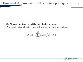
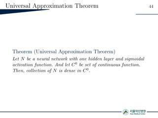
42. Universal Approximation Theorem - prerequisite 42
2. Sigmoidal function
A sigmoidal function is a monotonically increasing continuous
function σ : R → [0, 1] s.t.
σ(x) =
1 x → +∞
0 x → −∞

43. Universal Approximation Theorem - prerequisite 43
3. Neural network with one hidden layer
A neural network with one hidden layer is expressed as:
N(x) =
N
j=1
αjσ(yT
j x + θj)

44. Universal Approximation Theorem 44
Theorem (Universal Approximation Theorem)
Let N be a neural network with one hidden layer and sigmoidal
activation function. And let C0 be set of continuous function.
Then, collection of N is dense in C0.