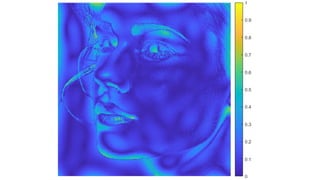
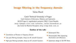
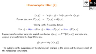
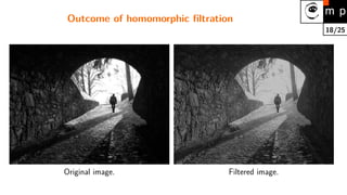
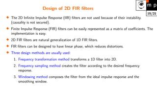
The document discusses various image filtering techniques in the frequency domain. It begins by introducing convolution as frequency domain filtering using the Fourier transform. It then provides examples of low pass and high pass filtering using sharp cut-off and Gaussian filters. Additional topics covered include the Butterworth filter, homomorphic filtering to separate illumination and reflectance, and systematic design of 2D finite impulse response (FIR) filters.

1. Image filtering in the frequency domain
Václav Hlaváč
Czech Technical University in Prague
Czech Institute of Informatics, Robotics and Cybernetics
160 00 Prague 6, Jugoslávských partyzánů 1580/3, Czech Republic
http://people.ciirc.cvut.cz/hlavac, vaclav.hlavac@cvut.cz
also Center for Machine Perception, http://cmp.felk.cvut.cz
Outline of the talk:
Convolution as filtration in frequency domain.
Low pass filtering examples, sharp cut off, smooth Gaussian.
High pass filtering examples, sharp cut off, smooth Gaussian.
Butterworth filter.
Homomorphic filter separating
illumination and reflectance.
Systematic design of 2D FIR filters.

2. 2/25
Filtration in the frequency domain
1. F(u, v) = F{f(x, y)}
2. G(u, v) = H(u, v) . ∗ F(u, v),
where .∗ denotes element-wise multiplication of matrices.
3. g(x, y) = F−1
{G(u, v)}
Note for lab exercises: We usually use ln kF(u, v)k for visualization purposes. The original
spectrum F(u, v) has to be used in the actual filtration.

3. 3/25
Convolution as Fourier spectrum frequency filtration
Matrix element by element multiplication.
The speed of operations is determined by the (high) speed of FFT.
Consider a matrix a with dimensions M × N and a matrix b with dimensions P × Q.
The convolution c = a ∗ b can be calculated as follows:
1. Fill in matrices a, b by zeroes to have dimensions M + P − 1, N + Q − 1 (usually up to the
order of 2 to ease FFT).
2. Calculate 2D FFT matic of matrices a, b (in MATLAB, using fft2). The outcome are
matrices A, B.
3. Multiply complex Fourier spectra element-wise, C = A . ∗ B.
4. The result of the convolution c is obtained by the inverse Fourier transformation (in MATLAB
using ifft2).

4. 4/25
2D convolution in frequency domain in MATLAB
A = magic(3);
B = ones(3);
A(8,8) = 0; % zero–pad A to be 8–by–8
B(8,8) = 0; % zero–pad B to be 8–by–8
C = ifft2(fft2(A).*fft2(B));
C = C(1:5,1:5); % extract the nonzero portion
C = real(C) % remove imaginary part caused by roundoff error
C =







8.0000 9.0000 15.0000 7.0000 6.0000
11.0000 17.0000 30.0000 19.0000 13.0000
15.0000 30.0000 45.0000 30.0000 15.0000
7.0000 21.0000 30.0000 23.0000 9.0000
4.0000 13.0000 15.0000 11.0000 2.0000







Note: the convolution calculated via spectra is faster in MATLAB for large matrices. The calculation via conv2,
filt2 is faster for small matrices.

5. 5/25
Low pass filter, circle sharp cut-off, r=5, 15, 50
original filter output in gray output in pseudocolor

6. 6/25
Low pass Gaussian filter, σ = 10, 30
original filter output in gray output in pseudocolor

7. 7/25
High pass circle sharp cut-off, r=5, 15
original filter output in gray output in pseudocolor

8. 8/25
High pass Gaussian filter, σ=10, 30
original filter output in gray output in pseudocolor

9. 9/25
Example, Fourier filtration, Gaussian filter

10. 10/25
Example, Fourier filtration, Sobel filter

11. 11/25
Example, Fourier filtration, Abs(Sobel filter)

12. 12/25
Low pass filter, Butterworth (1)
Butterworth filter has the frequency spectrum with the smallest rippling, which converges to zero
for maximal frequences (S. Buttherworth, 1930).
Shifted log(abs(FFT)) of the original image
200 400 600 800 1000
100
200
300
400
500
600
700
−2
0
2
4
6
8
10
12
Input image Its frequency spectrum

13. 13/25
Low pass filter, Butterworth (2)
Shifted log(abs(FFT)) of the filtered image
200 400 600 800 1000
100
200
300
400
500
600
700
−6
−4
−2
0
2
4
6
8
10
12
Butterworth low pass filter FFT of the filtered image
H(u, v) = 1
1+
D(u,v)
D0
2
n
, where D(u, v) =
√
u2 + v2. n is the filter degree.
D0 is the frequency corresponding to the decrease of intensity by 3dB.

14. 14/25
Low pass filter, Butterworth (3)
Input image Its frequency spectrum

15. 15/25
Homomorphic filter (1)
The aim: to normalize the intensity across the entire image and to increase contrast.
The method is based on the following assumptions:
Illumination i changes in the image very slowly (low frequencies),
Reflectance r changes in a more fast fashion, because the scene is usually rather diverse.
The image can be decomposed (factorized) in each pixel into a product of two components –
illumination i and reflectance r: f(x, y) = i(x, y) r(x, y).
The key idea: the logarithm function can be used to separate the illumination and the reflectance
components.

16. 16/25
Homomorphic filter (2)
z(x, y) = ln f(x, y) = ln i(x, y) + ln r(x, y)
Fourier spectrum Z(u, v) = I(u, v) + R(u, v)
Filtering in the frequency domain
S(u, v) = H(u, v)Z(u, v) = H(u, v)I(u, v) + H(u, v)R(u, v)
Inverse transformation back into spatial coordinates s(x, y) = F−1
{S(u, v)} and return to
original gray scale from the logarithmic one
g(x, y) = exp (s(x, y))
The outcome is the suppression in the illumination changes in the scene and the improvement of
the reflectance component.

17. 17/25
Homomorphic filters
50 100 150 200
0
0.2
0.4
0.6
0.8
1
1.2
1.4
homomorphic filter
Standard high−pass filter
Note: The filter is used to modify Z(u, v), not the original spectrum F(u, v)!

18. 18/25
Outcome of homomorphic filtration
Original image. Filtered image.

19. 19/25
Design of 2D FIR filters
The 2D Infinite Impulse Response (IIR) filters are not used because of their instability.
(causality is not secured).
Finite Impulse Response (FIR) filters can be easily represented as a matrix of coefficients. The
implementation is easy.
2D FIR filters are natural generalization of 1D FIR filters.
FIR filters can be designed to have linear phase, which reduces distortions.
Three design methods are usually used:
1. Frequency transformation method transforms a 1D filter into 2D.
2. Frequency sampling method creates the filter according to the desired frequency
response.
3. Windowing method composes the filter from the ideal impulse response and the
smoothing window.

20. 20/25
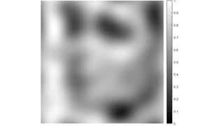
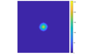
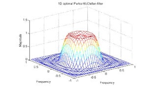
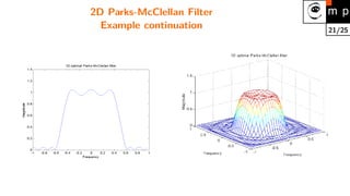
Frequency transformation method
The established methods for designing 1D filters can be used. The 1D filter is converted into 2D
by making the filter center symmetric. A good method.
A MATLAB example (Parks-McClellan optimal design):
b = remez(10,[0 0.4 0.6 1],[1 1 0 0]);
h = ftrans2(b);
[H,w] = freqz(b,1,64,’whole’);
colormap(jet(64))
plot(w/pi–1,fftshift(abs(H))) figure, freqz2(h,[32 32])

21. 21/25
2D Parks-McClellan Filter
Example continuation

22. 22/25
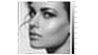
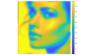
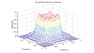
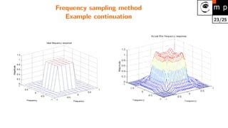
Frequency sampling method
The desired frequency response is given. The filter is created in the matrix form securing that the
response passes given frequency response points. The behavior can be arbitrary outside the given
points. Oscillations are common.
MATLAB example (design of the 11 × 11 filter)
Hd = zeros(11,11); Hd(4:8,4:8) = 1;
[f1,f2] = freqspace(11,’meshgrid’);
mesh(f1,f2,Hd), axis([-1 1 -1 1 0 1.2]), colormap(jet(64))
h = fsamp2(Hd);
figure, freqz2(h,[32 32]), axis([-1 1 –1 1 0 1.2])

23. 23/25
Frequency sampling method
Example continuation

24. 24/25
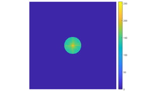
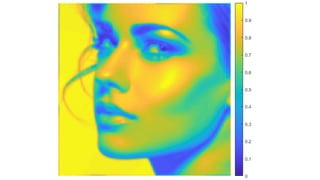
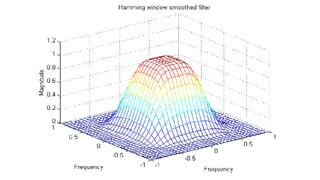
Windowing method
The ideal response of the filter smoothes the coefficients in the windos. The ideal filter is
approximated.
The results are usually better than the results of the Frequency Sampling Method.
Hd = zeros(11,11); Hd(4:8,4:8) = 1;
[f1,f2] = freqspace(11,’meshgrid’);
mesh(f1,f2,Hd), axis([–1 1 –1 1 0 1.2]), colormap(jet(64))
h = fwind1(Hd,hamming(11));
figure, freqz2(h,[32 32]), axis([–1 1 –1 1 0 1.2])

25. 25/25
Windowing method
Example continuation

76. Shifted log(abs(FFT)) of the original image
200 400 600 800 1000
100
200
300
400
500
600
700
−2
0
2
4
6
8
10
12

78. Shifted log(abs(FFT)) of the filtered image
200 400 600 800 1000
100
200
300
400
500
600
700
−6
−4
−2
0
2
4
6
8
10
12

82. 50 100 150 200
0
0.2
0.4
0.6
0.8
1
1.2
1.4
homomorphic filter
Standard high−pass filter