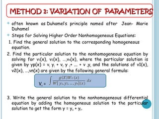
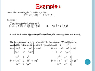
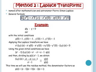
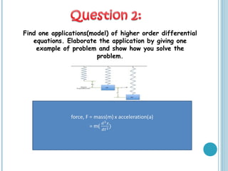
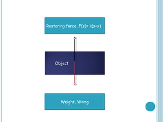
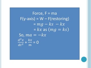
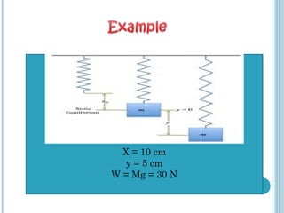
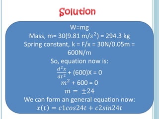
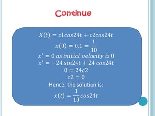
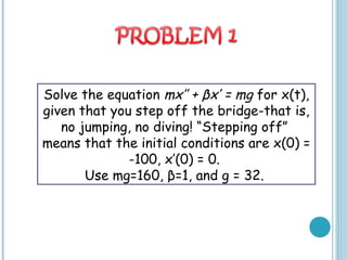
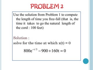
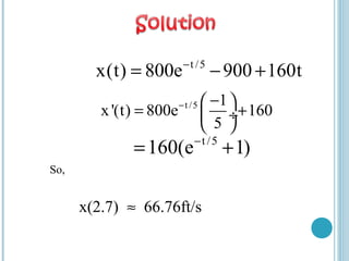
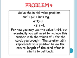
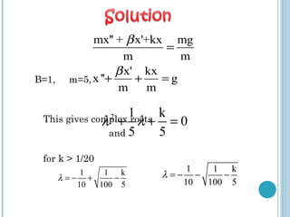
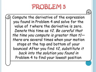
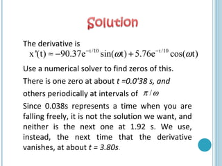
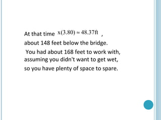
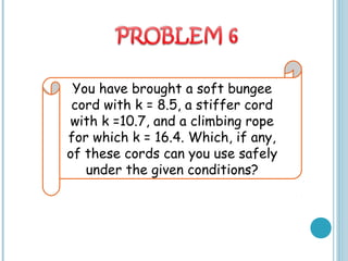
ORDINARY DIFFERENTIAL
EQUATION
SMN3043
ASSIGNMENT 2 PRESENTATION
SEMESTER : 6
PROGRAM : AT16 (PENDIDIKAN SAINS)
LECTURER NAME : CIK FAINIDA BINTI RAHMAT
NAME MATRIC NO.
NUR FARALINA BINTI ASRAB ALI D20101037415
NOOR AZURAH BT ABD RAZAK D20101037502
KESAVARTINII A/P BALA KRISNAIN D20101039444
JASMAN BIN RONIE D20101037474
Find two methods
(other than Undetermined Coefficients)
that can be used to solve higher order ODE.
For each method, solve one higher order ODE.
2 Methods : Variation of Parameters Laplace
Transforms
 often known as Duhamel’s principle named after  Jean- Marie
Duhamel
 Steps for Solving Higher Order Nonhomogeneous Equations:
1. Find the general solution to the corresponding homogeneous
equation.
2. Find the particular solution to the nonhomogeneous equation by
solving for v1(x), v2(x), …,vn(x), where the particular solution is
given by yp(x) = v1 y1 + v2 y 2+ ... + v nyn and the solutions of v1(x),
v2(x), …,vn(x) are given by the following general formula:
Vn =
3. Write the general solution to the nonhomogeneous differential
equation by adding the homogeneous solution to the particular
solution to get the form y = yH + yP.
METHOD 1: VARIATION OF PARAMETERSMETHOD 1: VARIATION OF PARAMETERS
Example :Example :
Solve the following differential equation.
                                                
Solution
The characteristic equation is,
      
So we have three real distinct roots here and so the general solution is,
We have now got several determinants to compute.  We will have to
verify the following determinant computations.
Now, given that    we can compute
each of the   .  Here are those integrals.
Finally, a particular solution for this differential
equation is then,
The general solution is then,
Method 2 : Laplace TransformsMethod 2 : Laplace Transforms
 named after mathematician and astronomer Pierre-Simon Laplace
 General formula:
Example:Example:
d4
y - y = 0
dx4
with the initial conditions
y(0) = 1 , y’(0) = -1 , y’’(0) = 1 , y’’’(0) = -1
Applying the Laplace transform we have
s4
(Ly) (s) - s3
y(0) - s2
y’(0) - s y’’(0) – y’’’(0) - (Ly) (s) = 0
Using the given initial conditions we have
(s4
- 1) (Ly) (s) = s3
- s2
+ s - 1 q(s)
and then, dividing by p(s) s4
- 1, we obtain
(Ly) (s) = s3
- s2
+ s – 1 q(s)
s4
– 1 p(s)
This time we will use the residue method; the denominator factors as
p(s) = (s - 1)(s + 1)(s - i)(s + i):
Thus we want s3
- s2
+ s – 1 =
s4
– 1
The residue formula then gives
C1 =
C2 =
C3 =
Then, c3 = 0 also and we have
(Ly) (s) = 1 y(x) =
s + 1
This was quick and almost trivial, so let's try another set of initial
conditions:
y(0) = 0 , y’(0) = 0, y’’(0) = 0, y’’’(0) = 1
This case gives q(s) 1. So now we have.
C1=
C3 =
(Ly) (s) =
=
y(x) =
=
Find one applications(model) of higher order differential
equations. Elaborate the application by giving one
example of problem and show how you solve the
problem.
Object
Restoring force, F(s)= k(s+x)
Weight, W=mg
X = 10 cm
y = 5 cm
W = Mg = 30 N
Solve the equation mx’’ + βx’ = mg for x(t),
given that you step off the bridge-that is,
no jumping, no diving! “Stepping off”
means that the initial conditions are x(0) =
-100, x’(0) = 0.
Use mg=160, β=1, and g = 32.
Given β= 1, and mg = 160 with g =32
So, m = 5
the characteristic polynomial for the homogeneous
equation is ,
So,
mx'' + x' mg
m m
x'
x'' g
m
β
β
=
+ =
2 1
0
5
λ λ+ =
with roots λ = 0 and λ= -1/5.
The forcing function due to gravity gives a solution of
form xp(t) = mgt - 160t,
Hence, we conclude that the formal solution is
t/5
x(t) Ae B 160t−
= + +
Now x(0) = -100 so A+ B = -100,
x'(0) = 0 implies A/5 = 160.
Thus, A = 800 and B = -900, so
t /5
x(t) 800e 900 160t−
= − +
Use the solution from Problem 1 to compute
the length of time you free-fall (that is, the
time it takes to go the natural length of
the cord : 100 feet)
Solution :
solve for the time at which x(t) = 0
t /5
800e 900 160t 0−
− + =
Compute the derivative of the
solution you found in Problem 1 and
evaluate it at the time you found in
Problem 2. You have found your
downward speed when you pass the
point where the cord starts to pull.
So,
x(2.7) 66.76ft/s≈
t /5
x(t) 800e 900 160t−
= − +
t /5 1
x'(t) 800e 160
5
− − 
= + ÷
 
t /5
160(e 1)−
= +
Solve the initial-value problem
mx’’ + βx’ + kx = mg,
x(t1)=0,
x’(t)=v1.
For now you may use the value k =14, but
eventually you will need to replace this
number with the values of k for the
cords you brought. The solution x(t)
represents your position below the
natural length of the cord after it
starts to pull back.
B=1, m=5,
This gives complex roots
and
for k > 1/20
mx'' + x'+kx mg
m m
x' kx
x'' g
m m
β
β
=
+ + =
2 1 k
0
5 5
λ λ+ + =
1 1 k
10 100 5
λ = − + −
1 1 k
10 100 5
λ = − − −
Thus, the formal solution to the homogenous
equation is
Xh(t)=Ae-t/10
sin(ωt) + βe-t/10
cos(ωt)
for
Using xp(t) =C, giving the equation kC = mg or
xp(t) =C= mg/k
Substitute the initial condition x(2.73)= 0 to
find that
x(t1)=Ae-t/10
sin(t1 ω) + βe-t/10
cos(t1ω)+ 160/k =0
1/100 k /5ω = − +
Take the derivative and use the other initial
condition to see that
Note that x(t1)=0
Thus, we have two simple simultaneous
equations to solve for A and B: given
any k.
When k= 14, then so,
and
t1/101 160
x(t1) - + e (Acos (t1 ) - B sin(t1 )) = 67.26
10 k
ω ω ω−−  
 ÷
 
1.67ω ≈ t1/10
e sin(t1 ) 0.75ω−
≈ −
t1/10
e cos(t1 ) 0.12ω−
≈ −
The system becomes approximately
We solve this to arrive at a solution
given approximately by
-160
-0.75A - 0.12B =
14
160
-0.20 A +0.75 B = 67.26 -
140
ω ω
t1/10 t1/10 160
x(t)=66e sin( t) 53e cos( t)
140
ω ω− −
+ +
In general, given k we compute
and then compute a11=e-t/10
sin (t1w) and
a12=e-t/10
cos (t1w)
We then solve the system
a11A+ a12B= -160/k
a12ωA- a11ωB=67.26-(160/10k)
to find the solution to the initial-value
problem.
k /5 0.1ω = −
Compute the derivative of the expression
you found in Problem 4 and solve for the
value of t where the derivative is zero.
Denote this time as t2. Be careful that
the time you compute is greater than t1—
there are several times when your motion
stops at the top and bottom of your
bounces! After you find t2, substitute it
back into the solution you found in
Problem 4 to find your lowest position
The derivative is
Use a numerical solver to find zeros of this.
There is one zero at about t =0.0'38 s, and
others periodically at intervals of
Since 0.038s represents a time when you are
falling freely, it is not the solution we want, and
neither is the next one at 1.92 s. We use,
instead, the next time that the derivative
vanishes, at about t = 3.80s.
t /10 t /10
x'(t) 90.37e sin( t) 5.76e cos( t)ω ω− −
≈ − +
/π ω
At that time ,
about 148 feet below the bridge.
You had about 168 feet to work with,
assuming you didn't want to get wet,
so you have plenty of space to spare.
x(3.80) 48.37ft≈
You have brought a soft bungee
cord with k = 8.5, a stiffer cord
with k =10.7, and a climbing rope
for which k = 16.4. Which, if any,
of these cords can you use safely
under the given conditions?
We use the tool that have been given by our lecturer which can
help us plot the solution of the given k values to identify which
of them allow to hit the water. The cord type can probably use
any of the bungee cords given with safety. In the tool, it has
been set up using the stiffer cord, hence I just change the k
values, though the one with k = 8.5 will almost get wet.
k values ≈8.5 k values ≈ 10.7 k values = 16.4
Figure show the position of the path
of each k values.
From the figures we can make a conclusion that the
position of the k = 8.5 had almost reached the water
compare to the others values and had indicate the
relevant path as the jumper approaches the water.
You have a bungee cord for which you
have not determined the spring
constant k. To do so, you suspend a
weight of 10 pounds from the end of
the 100-foot cord, causing it to
stretch 1.2 feet. What is the value of
k for this cord?
You have a bungee cord for which you
have not determined the spring
constant k. To do so, you suspend a
weight of 10 pounds from the end of
the 100-foot cord, causing it to
stretch 1.2 feet. What is the value of
k for this cord?
Let, mg =10.
When the weight comes to
rest, we can assume x’ = x”= 0.
So kx = mg.
As we know from the question,
the weight has stretched the
cord by 1.2 ft.
Hence we can conclude that,
k(1.2) = 10 or k ≈ 8.3
What would happen if
your 220-pound friend
uses the bungee cord
whose spring constant
is k=10.7?
When my 220 pound and probably 6 feet tall friend uses
the bungee cord, at the end of the cord scrapes the
water, he is quite wet.
If the water is not deep, he had better not take the
chance on this jump.
He can, however, survive the jump on the cord with k = 14.
Figure/graph below show the position of the friend when
he jumps.
If your heavy friend
wants to jump anyway,
then how short should
you make the cord so
that he does not get
wet?
Using the tool given we can indicates the length of the
cord to make sure he does not wet.
When the cord is shortened to about 96 feet
(Let the initial condition is changed to x(O) = -96).
Then our friend seems to be able to jump without getting
more than a few hairs wet.
 Dennis G. Zill, Warren S. Wright, Michael R. Cullen. ( 2012). Differential Equations With
Boundary-Value Problems. (Vol 8, pp. 12, 116-128). USA. Cengage Learning.
 Kristensson, G. (2010). Second order differential equations. (Vol 1). London. Springer New York.
 Dyke, P.P.G. (1999). An Introduction to Laplace Transforms and Fourier Series: With 51 Figures
(pp. 54-63). Britain. Athenaeum Press Ltd, Gateshead, Tyne & Wear.
 Paul Dawkins(2013). Paul's Online Math Notes. Retrieved on April 31, 2013 from
http://tutorial.math.lamar.edu/Classes/DE/HOVariationOfParam.aspx
Method of Variation of Parameters (Higher Order) (2013). Retrieved on April 31, 2013 from
http://www.utdallas.edu/dept/abp/PDF_Files/DE_Folder/VariationofParametersII.pdf
 Laplace Solution of Initial Value Problems (2013). Retrieved on April 31, 2013 from
http://www.math.vt.edu/people/dlr/m2k_opm_slvint.pdf
 Laplace transform (2013). Retrieved on April 31, 2013 from
http://en.wikipedia.org/wiki/Laplace_transform
Ordinary Differential Equation

Ordinary Differential Equation

  • 1.
    ORDINARY DIFFERENTIAL EQUATION SMN3043 ASSIGNMENT 2PRESENTATION SEMESTER : 6 PROGRAM : AT16 (PENDIDIKAN SAINS) LECTURER NAME : CIK FAINIDA BINTI RAHMAT NAME MATRIC NO. NUR FARALINA BINTI ASRAB ALI D20101037415 NOOR AZURAH BT ABD RAZAK D20101037502 KESAVARTINII A/P BALA KRISNAIN D20101039444 JASMAN BIN RONIE D20101037474
  • 2.
    Find two methods (otherthan Undetermined Coefficients) that can be used to solve higher order ODE. For each method, solve one higher order ODE. 2 Methods : Variation of Parameters Laplace Transforms
  • 3.
     often knownas Duhamel’s principle named after  Jean- Marie Duhamel  Steps for Solving Higher Order Nonhomogeneous Equations: 1. Find the general solution to the corresponding homogeneous equation. 2. Find the particular solution to the nonhomogeneous equation by solving for v1(x), v2(x), …,vn(x), where the particular solution is given by yp(x) = v1 y1 + v2 y 2+ ... + v nyn and the solutions of v1(x), v2(x), …,vn(x) are given by the following general formula: Vn = 3. Write the general solution to the nonhomogeneous differential equation by adding the homogeneous solution to the particular solution to get the form y = yH + yP. METHOD 1: VARIATION OF PARAMETERSMETHOD 1: VARIATION OF PARAMETERS
  • 4.
    Example :Example : Solvethe following differential equation.                                                  Solution The characteristic equation is,        So we have three real distinct roots here and so the general solution is, We have now got several determinants to compute.  We will have to verify the following determinant computations.
  • 5.
    Now, given that   we can compute each of the   .  Here are those integrals. Finally, a particular solution for this differential equation is then, The general solution is then,
  • 6.
    Method 2 :Laplace TransformsMethod 2 : Laplace Transforms  named after mathematician and astronomer Pierre-Simon Laplace  General formula: Example:Example: d4 y - y = 0 dx4 with the initial conditions y(0) = 1 , y’(0) = -1 , y’’(0) = 1 , y’’’(0) = -1 Applying the Laplace transform we have s4 (Ly) (s) - s3 y(0) - s2 y’(0) - s y’’(0) – y’’’(0) - (Ly) (s) = 0 Using the given initial conditions we have (s4 - 1) (Ly) (s) = s3 - s2 + s - 1 q(s) and then, dividing by p(s) s4 - 1, we obtain (Ly) (s) = s3 - s2 + s – 1 q(s) s4 – 1 p(s) This time we will use the residue method; the denominator factors as p(s) = (s - 1)(s + 1)(s - i)(s + i):
  • 7.
    Thus we wants3 - s2 + s – 1 = s4 – 1 The residue formula then gives C1 = C2 = C3 = Then, c3 = 0 also and we have (Ly) (s) = 1 y(x) = s + 1 This was quick and almost trivial, so let's try another set of initial conditions: y(0) = 0 , y’(0) = 0, y’’(0) = 0, y’’’(0) = 1 This case gives q(s) 1. So now we have.
  • 8.
    C1= C3 = (Ly) (s)= = y(x) = =
  • 9.
    Find one applications(model)of higher order differential equations. Elaborate the application by giving one example of problem and show how you solve the problem.
  • 10.
    Object Restoring force, F(s)=k(s+x) Weight, W=mg
  • 12.
    X = 10cm y = 5 cm W = Mg = 30 N
  • 16.
    Solve the equationmx’’ + βx’ = mg for x(t), given that you step off the bridge-that is, no jumping, no diving! “Stepping off” means that the initial conditions are x(0) = -100, x’(0) = 0. Use mg=160, β=1, and g = 32.
  • 17.
    Given β= 1,and mg = 160 with g =32 So, m = 5 the characteristic polynomial for the homogeneous equation is , So, mx'' + x' mg m m x' x'' g m β β = + = 2 1 0 5 λ λ+ =
  • 18.
    with roots λ= 0 and λ= -1/5. The forcing function due to gravity gives a solution of form xp(t) = mgt - 160t, Hence, we conclude that the formal solution is t/5 x(t) Ae B 160t− = + +
  • 19.
    Now x(0) =-100 so A+ B = -100, x'(0) = 0 implies A/5 = 160. Thus, A = 800 and B = -900, so t /5 x(t) 800e 900 160t− = − +
  • 20.
    Use the solutionfrom Problem 1 to compute the length of time you free-fall (that is, the time it takes to go the natural length of the cord : 100 feet) Solution : solve for the time at which x(t) = 0 t /5 800e 900 160t 0− − + =
  • 21.
    Compute the derivativeof the solution you found in Problem 1 and evaluate it at the time you found in Problem 2. You have found your downward speed when you pass the point where the cord starts to pull.
  • 22.
    So, x(2.7) 66.76ft/s≈ t /5 x(t)800e 900 160t− = − + t /5 1 x'(t) 800e 160 5 − −  = + ÷   t /5 160(e 1)− = +
  • 23.
    Solve the initial-valueproblem mx’’ + βx’ + kx = mg, x(t1)=0, x’(t)=v1. For now you may use the value k =14, but eventually you will need to replace this number with the values of k for the cords you brought. The solution x(t) represents your position below the natural length of the cord after it starts to pull back.
  • 24.
    B=1, m=5, This givescomplex roots and for k > 1/20 mx'' + x'+kx mg m m x' kx x'' g m m β β = + + = 2 1 k 0 5 5 λ λ+ + = 1 1 k 10 100 5 λ = − + − 1 1 k 10 100 5 λ = − − −
  • 25.
    Thus, the formalsolution to the homogenous equation is Xh(t)=Ae-t/10 sin(ωt) + βe-t/10 cos(ωt) for Using xp(t) =C, giving the equation kC = mg or xp(t) =C= mg/k Substitute the initial condition x(2.73)= 0 to find that x(t1)=Ae-t/10 sin(t1 ω) + βe-t/10 cos(t1ω)+ 160/k =0 1/100 k /5ω = − +
  • 26.
    Take the derivativeand use the other initial condition to see that Note that x(t1)=0 Thus, we have two simple simultaneous equations to solve for A and B: given any k. When k= 14, then so, and t1/101 160 x(t1) - + e (Acos (t1 ) - B sin(t1 )) = 67.26 10 k ω ω ω−−    ÷   1.67ω ≈ t1/10 e sin(t1 ) 0.75ω− ≈ − t1/10 e cos(t1 ) 0.12ω− ≈ −
  • 27.
    The system becomesapproximately We solve this to arrive at a solution given approximately by -160 -0.75A - 0.12B = 14 160 -0.20 A +0.75 B = 67.26 - 140 ω ω t1/10 t1/10 160 x(t)=66e sin( t) 53e cos( t) 140 ω ω− − + +
  • 28.
    In general, givenk we compute and then compute a11=e-t/10 sin (t1w) and a12=e-t/10 cos (t1w) We then solve the system a11A+ a12B= -160/k a12ωA- a11ωB=67.26-(160/10k) to find the solution to the initial-value problem. k /5 0.1ω = −
  • 29.
    Compute the derivativeof the expression you found in Problem 4 and solve for the value of t where the derivative is zero. Denote this time as t2. Be careful that the time you compute is greater than t1— there are several times when your motion stops at the top and bottom of your bounces! After you find t2, substitute it back into the solution you found in Problem 4 to find your lowest position
  • 30.
    The derivative is Usea numerical solver to find zeros of this. There is one zero at about t =0.0'38 s, and others periodically at intervals of Since 0.038s represents a time when you are falling freely, it is not the solution we want, and neither is the next one at 1.92 s. We use, instead, the next time that the derivative vanishes, at about t = 3.80s. t /10 t /10 x'(t) 90.37e sin( t) 5.76e cos( t)ω ω− − ≈ − + /π ω
  • 31.
    At that time, about 148 feet below the bridge. You had about 168 feet to work with, assuming you didn't want to get wet, so you have plenty of space to spare. x(3.80) 48.37ft≈
  • 32.
    You have broughta soft bungee cord with k = 8.5, a stiffer cord with k =10.7, and a climbing rope for which k = 16.4. Which, if any, of these cords can you use safely under the given conditions?
  • 33.
    We use thetool that have been given by our lecturer which can help us plot the solution of the given k values to identify which of them allow to hit the water. The cord type can probably use any of the bungee cords given with safety. In the tool, it has been set up using the stiffer cord, hence I just change the k values, though the one with k = 8.5 will almost get wet.
  • 34.
    k values ≈8.5k values ≈ 10.7 k values = 16.4 Figure show the position of the path of each k values. From the figures we can make a conclusion that the position of the k = 8.5 had almost reached the water compare to the others values and had indicate the relevant path as the jumper approaches the water.
  • 35.
    You have abungee cord for which you have not determined the spring constant k. To do so, you suspend a weight of 10 pounds from the end of the 100-foot cord, causing it to stretch 1.2 feet. What is the value of k for this cord? You have a bungee cord for which you have not determined the spring constant k. To do so, you suspend a weight of 10 pounds from the end of the 100-foot cord, causing it to stretch 1.2 feet. What is the value of k for this cord?
  • 36.
    Let, mg =10. Whenthe weight comes to rest, we can assume x’ = x”= 0. So kx = mg. As we know from the question, the weight has stretched the cord by 1.2 ft. Hence we can conclude that, k(1.2) = 10 or k ≈ 8.3
  • 37.
    What would happenif your 220-pound friend uses the bungee cord whose spring constant is k=10.7?
  • 38.
    When my 220pound and probably 6 feet tall friend uses the bungee cord, at the end of the cord scrapes the water, he is quite wet. If the water is not deep, he had better not take the chance on this jump. He can, however, survive the jump on the cord with k = 14. Figure/graph below show the position of the friend when he jumps.
  • 39.
    If your heavyfriend wants to jump anyway, then how short should you make the cord so that he does not get wet?
  • 40.
    Using the toolgiven we can indicates the length of the cord to make sure he does not wet. When the cord is shortened to about 96 feet (Let the initial condition is changed to x(O) = -96). Then our friend seems to be able to jump without getting more than a few hairs wet.
  • 41.
     Dennis G.Zill, Warren S. Wright, Michael R. Cullen. ( 2012). Differential Equations With Boundary-Value Problems. (Vol 8, pp. 12, 116-128). USA. Cengage Learning.  Kristensson, G. (2010). Second order differential equations. (Vol 1). London. Springer New York.  Dyke, P.P.G. (1999). An Introduction to Laplace Transforms and Fourier Series: With 51 Figures (pp. 54-63). Britain. Athenaeum Press Ltd, Gateshead, Tyne & Wear.  Paul Dawkins(2013). Paul's Online Math Notes. Retrieved on April 31, 2013 from http://tutorial.math.lamar.edu/Classes/DE/HOVariationOfParam.aspx Method of Variation of Parameters (Higher Order) (2013). Retrieved on April 31, 2013 from http://www.utdallas.edu/dept/abp/PDF_Files/DE_Folder/VariationofParametersII.pdf  Laplace Solution of Initial Value Problems (2013). Retrieved on April 31, 2013 from http://www.math.vt.edu/people/dlr/m2k_opm_slvint.pdf  Laplace transform (2013). Retrieved on April 31, 2013 from http://en.wikipedia.org/wiki/Laplace_transform