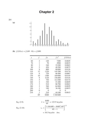
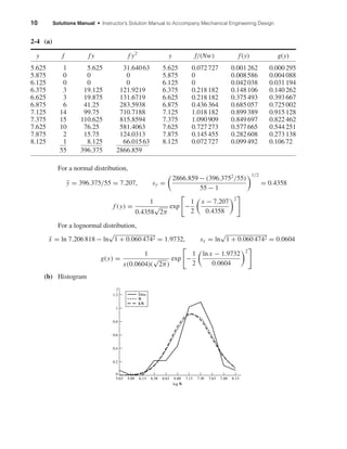
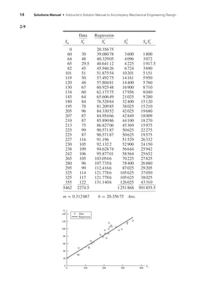
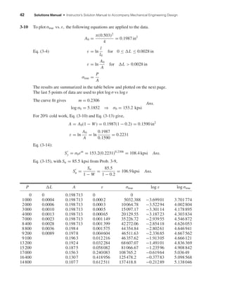
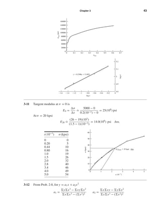
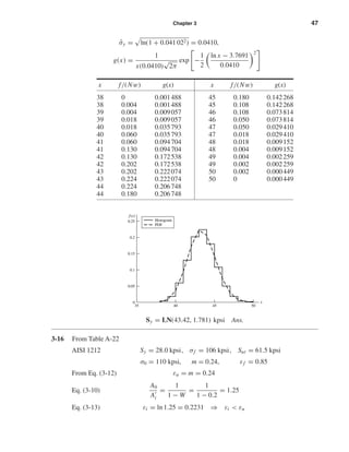
This document provides equations and calculations for determining the mean cycles to failure (x-bar) and standard deviation (s_x) of fatigue test data. The given data shows cycles to failure (x) from fatigue tests of a material at various stress levels (f). The mean x-bar is calculated as 122.9 kcycles using equation 2-9. The standard deviation s_x is calculated as 30.3 kcycles using equation 2-10.

1. Chapter 1
D
B
G
F
Facc
A
E
f f
1 1
␪cr
␪
C
Impending motion to left
Fcr
Consider force F at G, reactions at B and D. Extend lines of action for fully-developed fric-
tion DE and BE to find the point of concurrency at E for impending motion to the left. The
critical angle is θcr. Resolve force F into components Facc and Fcr. Facc is related to mass and
acceleration. Pin accelerates to left for any angle 0 < θ < θcr. When θ > θcr, no magnitude
of F will move the pin.
D
B
G
FЈ
FЈacc
A
EЈ иE
f f
1 1
C
d
Impending motion to right
␪Ј
FcrЈ
␪crЈ
Consider force F at G, reactions at A and C. Extend lines of action for fully-developed fric-
tion AE and C E to find the point of concurrency at E for impending motion to the left. The
critical angle is θcr. Resolve force F into components Facc and Fcr. Facc is related to mass
and acceleration. Pin accelerates to right for any angle 0 < θ < θcr. When θ > θcr, no mag-
nitude of F will move the pin.
The intent of the question is to get the student to draw and understand the free body in
order to recognize what it teaches. The graphic approach accomplishes this quickly. It is im-
portant to point out that this understanding enables a mathematical model to be constructed,
and that there are two of them.
This is the simplest problem in mechanical engineering. Using it is a good way to begin a
course.
What is the role of pin diameter d?
Yes, changing the sense of F changes the response.
Problems 1-1 through 1-4 are for student research.
1-5
shi20396_ch01.qxd 6/5/03 12:11 PM Page 1

2. 2 Solutions Manual • Instructor’s Solution Manual to Accompany Mechanical Engineering Design
1-6
(a) Fy = −F − f N cos θ + N sin θ = 0 (1)
Fx = f N sin θ + N cos θ −
T
r
= 0
F = N(sin θ − f cos θ) Ans.
T = Nr( f sin θ + cos θ)
Combining
T = Fr
1 + f tan θ
tan θ − f
= KFr Ans. (2)
(b) If T → ∞ detent self-locking tan θ − f = 0 ∴ θcr = tan−1
f Ans.
(Friction is fully developed.)
Check: If F = 10 lbf, f = 0.20, θ = 45◦, r = 2 in
N =
10
−0.20 cos 45◦ + sin 45◦
= 17.68 lbf
T
r
= 17.28(0.20 sin 45◦
+ cos 45◦
) = 15 lbf
f N = 0.20(17.28) = 3.54 lbf
θcr = tan−1
f = tan−1
(0.20) = 11.31◦
11.31° < θ < 90°
1-7
(a) F = F0 + k(0) = F0
T1 = F0r Ans.
(b) When teeth are about to clear
F = F0 + kx2
From Prob. 1-6
T2 = Fr
f tan θ + 1
tan θ − f
T2 = r
(F0 + kx2)( f tan θ + 1)
tan θ − f
Ans.
1-8
Given, F = 10 + 2.5x lbf, r = 2 in, h = 0.2 in, θ = 60◦
, f = 0.25, xi = 0, xf = 0.2
Fi = 10 lbf; Ff = 10 + 2.5(0.2) = 10.5 lbf Ans.
x
y
F
fN
N
␪
T
r
shi20396_ch01.qxd 6/5/03 12:11 PM Page 2

3. Chapter 1 3
From Eq. (1) of Prob. 1-6
N =
F
− f cos θ + sin θ
Ni =
10
−0.25 cos 60◦ + sin 60◦
= 13.49 lbf Ans.
Nf =
10.5
10
13.49 = 14.17 lbf Ans.
From Eq. (2) of Prob. 1-6
K =
1 + f tan θ
tan θ − f
=
1 + 0.25 tan 60◦
tan 60◦ − 0.25
= 0.967 Ans.
Ti = 0.967(10)(2) = 19.33 lbf · in
Tf = 0.967(10.5)(2) = 20.31 lbf · in
1-9
(a) Point vehicles
Q =
cars
hour
=
v
x
=
42.1v − v2
0.324
Seek stationary point maximum
dQ
dv
= 0 =
42.1 − 2v
0.324
∴ v* = 21.05 mph
Q* =
42.1(21.05) − 21.052
0.324
= 1367.6 cars/h Ans.
(b)
Q =
v
x + l
=
0.324
v(42.1) − v2
+
l
v
−1
Maximize Q with l = 10/5280 mi
v Q
22.18 1221.431
22.19 1221.433
22.20 1221.435 ←
22.21 1221.435
22.22 1221.434
% loss of throughput
1368 − 1221
1221
= 12% Ans.
xl
2
l
2
v
x
v
shi20396_ch01.qxd 6/5/03 12:11 PM Page 3

4. 4 Solutions Manual • Instructor’s Solution Manual to Accompany Mechanical Engineering Design
(c) % increase in speed
22.2 − 21.05
21.05
= 5.5%
Modest change in optimal speed Ans.
1-10 This and the following problem may be the student’s first experience with a figure of merit.
• Formulate fom to reflect larger figure of merit for larger merit.
• Use a maximization optimization algorithm. When one gets into computer implementa-
tion and answers are not known, minimizing instead of maximizing is the largest error
one can make.
FV = F1 sin θ − W = 0
FH = −F1 cos θ − F2 = 0
From which
F1 = W/sin θ
F2 = −W cos θ/sin θ
fom = −S = −¢γ (volume)
.
= −¢γ(l1 A1 + l2 A2)
A1 =
F1
S
=
W
S sin θ
, l2 =
l1
cos θ
A2 =
F2
S
=
W cos θ
S sin θ
fom = −¢γ
l2
cos θ
W
S sin θ
+
l2W cos θ
S sin θ
=
−¢γ Wl2
S
1 + cos2
θ
cos θ sin θ
Set leading constant to unity
θ◦ fom
0 −∞
20 −5.86
30 −4.04
40 −3.22
45 −3.00
50 −2.87
54.736 −2.828
60 −2.886
Check second derivative to see if a maximum, minimum, or point of inflection has been
found. Or, evaluate fom on either side of θ*.
θ* = 54.736◦
Ans.
fom* = −2.828
Alternative:
d
dθ
1 + cos2
θ
cos θ sin θ
= 0
And solve resulting tran-
scendental for θ*.
shi20396_ch01.qxd 6/5/03 12:11 PM Page 4

5. Chapter 1 5
1-11
(a) x1 + x2 = X1 + e1 + X2 + e2
error = e = (x1 + x2) − (X1 + X2)
= e1 + e2 Ans.
(b) x1 − x2 = X1 + e1 − (X2 + e2)
e = (x1 − x2) − (X1 − X2) = e1 − e2 Ans.
(c) x1x2 = (X1 + e1)(X2 + e2)
e = x1x2 − X1 X2 = X1e2 + X2e1 + e1e2
.
= X1e2 + X2e1 = X1 X2
e1
X1
+
e2
X2
Ans.
(d)
x1
x2
=
X1 + e1
X2 + e2
=
X1
X2
1 + e1/X1
1 + e2/X2
1 +
e2
X2
−1
.
= 1 −
e2
X2
and 1 +
e1
X1
1 −
e2
X2
.
= 1 +
e1
X1
−
e2
X2
e =
x1
x2
−
X1
X2
.
=
X1
X2
e1
X1
−
e2
X2
Ans.
1-12
(a) x1 =
√
5 = 2.236 067 977 5
X1 = 2.23 3-correct digits
x2 =
√
6 = 2.449 487 742 78
X2 = 2.44 3-correct digits
x1 + x2 =
√
5 +
√
6 = 4.685 557 720 28
e1 = x1 − X1 =
√
5 − 2.23 = 0.006 067 977 5
e2 = x2 − X2 =
√
6 − 2.44 = 0.009 489 742 78
e = e1 + e2 =
√
5 − 2.23 +
√
6 − 2.44 = 0.015 557 720 28
Sum = x1 + x2 = X1 + X2 + e
= 2.23 + 2.44 + 0.015 557 720 28
= 4.685 557 720 28 (Checks) Ans.
(b) X1 = 2.24, X2 = 2.45
e1 =
√
5 − 2.24 = −0.003 932 022 50
e2 =
√
6 − 2.45 = −0.000 510 257 22
e = e1 + e2 = −0.004 442 279 72
Sum = X1 + X2 + e
= 2.24 + 2.45 + (−0.004 442 279 72)
= 4.685 557 720 28 Ans.
shi20396_ch01.qxd 6/5/03 12:11 PM Page 5

6. 6 Solutions Manual • Instructor’s Solution Manual to Accompany Mechanical Engineering Design
1-13
(a) σ = 20(6.89) = 137.8 MPa
(b) F = 350(4.45) = 1558 N = 1.558 kN
(c) M = 1200 lbf · in (0.113) = 135.6 N · m
(d) A = 2.4(645) = 1548 mm2
(e) I = 17.4 in4
(2.54)4
= 724.2 cm4
(f) A = 3.6(1.610)2
= 9.332 km2
(g) E = 21(1000)(6.89) = 144.69(103
) MPa = 144.7 GPa
(h) v = 45 mi/h (1.61) = 72.45 km/h
(i) V = 60 in3
(2.54)3
= 983.2 cm3
= 0.983 liter
1-14
(a) l = 1.5/0.305 = 4.918 ft = 59.02 in
(b) σ = 600/6.89 = 86.96 kpsi
(c) p = 160/6.89 = 23.22 psi
(d) Z = 1.84(105
)/(25.4)3
= 11.23 in3
(e) w = 38.1/175 = 0.218 lbf/in
(f) δ = 0.05/25.4 = 0.00197 in
(g) v = 6.12/0.0051 = 1200 ft/min
(h) = 0.0021 in/in
(i) V = 30/(0.254)3
= 1831 in3
1-15
(a) σ =
200
15.3
= 13.1 MPa
(b) σ =
42(103
)
6(10−2)2
= 70(106
) N/m2
= 70 MPa
(c) y =
1200(800)3
(10−3
)3
3(207)(6.4)(109)(10−2)4
= 1.546(10−2
) m = 15.5 mm
(d) θ =
1100(250)(10−3
)
79.3(π/32)(25)4(109)(10−3)4
= 9.043(10−2
) rad = 5.18◦
1-16
(a) σ =
600
20(6)
= 5 MPa
(b) I =
1
12
8(24)3
= 9216 mm4
(c) I =
π
64
324
(10−1
)4
= 5.147 cm4
(d) τ =
16(16)
π(253)(10−3)3
= 5.215(106
) N/m2
= 5.215 MPa
shi20396_ch01.qxd 6/5/03 12:11 PM Page 6

7. Chapter 1 7
1-17
(a) τ =
120(103
)
(π/4)(202)
= 382 MPa
(b) σ =
32(800)(800)(10−3
)
π(32)3(10−3)3
= 198.9(106
) N/m2
= 198.9 MPa
(c) Z =
π
32(36)
(364
− 264
) = 3334 mm3
(d) k =
(1.6)4
(79.3)(10−3
)4
(109
)
8(19.2)3(32)(10−3)3
= 286.8 N/m
shi20396_ch01.qxd 6/5/03 12:11 PM Page 7

8. (b) f/(N x) = f/(69 · 10) = f/690
Eq. (2-9) ¯x =
8480
69
= 122.9 kcycles
Eq. (2-10) sx =
1 104 600 − 84802
/69
69 − 1
1/2
= 30.3 kcycles Ans.
x f fx f x2
f/(N x)
60 2 120 7200 0.0029
70 1 70 4900 0.0015
80 3 240 19200 0.0043
90 5 450 40500 0.0072
100 8 800 80000 0.0116
110 12 1320 145200 0.0174
120 6 720 86400 0.0087
130 10 1300 169000 0.0145
140 8 1120 156800 0.0116
150 5 750 112500 0.0174
160 2 320 51200 0.0029
170 3 510 86700 0.0043
180 2 360 64 800 0.0029
190 1 190 36100 0.0015
200 0 0 0 0
210 1 210 44100 0.0015
69 8480 1104 600
Chapter 2
2-1
(a)
0
60 210190 200180170160150140130120110100908070
2
4
6
8
10
12
shi20396_ch02.qxd 7/21/03 3:28 PM Page 8

9. Chapter 2 9
2-2 Data represents a 7-class histogram with N = 197.
2-3
Form a table:
¯x =
4548
58
= 78.4 kpsi
sx =
359 088 − 45482
/58
58 − 1
1/2
= 6.57 kpsi
From Eq. (2-14)
f (x) =
1
6.57
√
2π
exp −
1
2
x − 78.4
6.57
2
x f fx f x2
64 2 128 8192
68 6 408 27744
72 6 432 31104
76 9 684 51984
80 19 1520 121600
84 10 840 70560
88 4 352 30976
92 2 184 16928
58 4548 359088
x f fx f x2
174 6 1044 181656
182 9 1638 298116
190 44 8360 1588400
198 67 13266 2626688
206 53 10918 2249108
214 12 2568 549552
220 6 1320 290400
197 39114 7789900
¯x =
39 114
197
= 198.55 kpsi Ans.
sx =
7 783 900 − 39 1142
/197
197 − 1
1/2
= 9.55 kpsi Ans.
shi20396_ch02.qxd 7/21/03 3:28 PM Page 9

10. 10 Solutions Manual • Instructor’s Solution Manual to Accompany Mechanical Engineering Design
2-4 (a)
y f fy f y2
y f/(Nw) f(y) g(y)
5.625 1 5.625 31.64063 5.625 0.072727 0.001262 0.000 295
5.875 0 0 0 5.875 0 0.008586 0.004 088
6.125 0 0 0 6.125 0 0.042038 0.031 194
6.375 3 19.125 121.9219 6.375 0.218182 0.148106 0.140 262
6.625 3 19.875 131.6719 6.625 0.218182 0.375493 0.393 667
6.875 6 41.25 283.5938 6.875 0.436364 0.685057 0.725 002
7.125 14 99.75 710.7188 7.125 1.018 182 0.899 389 0.915 128
7.375 15 110.625 815.8594 7.375 1.090 909 0.849 697 0.822 462
7.625 10 76.25 581.4063 7.625 0.727 273 0.577 665 0.544 251
7.875 2 15.75 124.0313 7.875 0.145455 0.282608 0.273 138
8.125 1 8.125 66.01563 8.125 0.072727 0.099492 0.10672
55 396.375 2866.859
For a normal distribution,
¯y = 396.375/55 = 7.207, sy =
2866.859 − (396.3752
/55)
55 − 1
1/2
= 0.4358
f (y) =
1
0.4358
√
2π
exp −
1
2
x − 7.207
0.4358
2
For a lognormal distribution,
¯x = ln 7.206 818 − ln
√
1 + 0.060 4742 = 1.9732, sx = ln
√
1 + 0.060 4742 = 0.0604
g(y) =
1
x(0.0604)(
√
2π)
exp −
1
2
ln x − 1.9732
0.0604
2
(b) Histogram
0
0.2
0.4
0.6
0.8
1
1.2
5.63 5.88 6.13 6.38 6.63 6.88
log N
7.13 7.38 7.63 7.88 8.13
Data
N
LN
f
shi20396_ch02.qxd 7/21/03 3:28 PM Page 10

11. Chapter 2 11
2-5 Distribution is uniform in interval 0.5000 to 0.5008 in, range numbers are a = 0.5000,
b = 0.5008 in.
(a) Eq. (2-22) µx =
a + b
2
=
0.5000 + 0.5008
2
= 0.5004
Eq. (2-23) σx =
b − a
2
√
3
=
0.5008 − 0.5000
2
√
3
= 0.000 231
(b) PDF from Eq. (2-20)
f (x) =
1250 0.5000 ≤ x ≤ 0.5008 in
0 otherwise
(c) CDF from Eq. (2-21)
F(x) =



0 x < 0.5000
(x − 0.5)/0.0008 0.5000 ≤ x ≤ 0.5008
1 x > 0.5008
If all smaller diameters are removed by inspection, a = 0.5002, b = 0.5008
µx =
0.5002 + 0.5008
2
= 0.5005 in
ˆσx =
0.5008 − 0.5002
2
√
3
= 0.000 173 in
f (x) =
1666.7 0.5002 ≤ x ≤ 0.5008
0 otherwise
F(x) =



0 x < 0.5002
1666.7(x − 0.5002) 0.5002 ≤ x ≤ 0.5008
1 x > 0.5008
2-6 Dimensions produced are due to tool dulling and wear. When parts are mixed, the distribution
is uniform. From Eqs. (2-22) and (2-23),
a = µx −
√
3s = 0.6241 −
√
3(0.000 581) = 0.6231 in
b = µx +
√
3s = 0.6241 +
√
3(0.000 581) = 0.6251 in
We suspect the dimension was
0.623
0.625
in Ans.
shi20396_ch02.qxd 7/21/03 3:28 PM Page 11

12. 12 Solutions Manual • Instructor’s Solution Manual to Accompany Mechanical Engineering Design
2-7 F(x) = 0.555x − 33 mm
(a) Since F(x) is linear, the distribution is uniform at x = a
F(a) = 0 = 0.555(a) − 33
∴ a = 59.46 mm. Therefore, at x = b
F(b) = 1 = 0.555b − 33
∴ b = 61.26 mm. Therefore,
F(x) =



0 x < 59.46 mm
0.555x − 33 59.46 ≤ x ≤ 61.26 mm
1 x > 61.26 mm
The PDF is dF/dx, thus the range numbers are:
f (x) =
0.555 59.46 ≤ x ≤ 61.26 mm
0 otherwise
Ans.
From the range numbers,
µx =
59.46 + 61.26
2
= 60.36 mm Ans.
ˆσx =
61.26 − 59.46
2
√
3
= 0.520 mm Ans.
1
(b) σ is an uncorrelated quotient ¯F = 3600 lbf, ¯A = 0.112 in2
CF = 300/3600 = 0.083 33, CA = 0.001/0.112 = 0.008 929
From Table 2-6, for σ
¯σ =
µF
µA
=
3600
0.112
= 32 143 psi Ans.
ˆσσ = 32 143
(0.083332
+ 0.0089292
)
(1 + 0.0089292)
1/2
= 2694 psi Ans.
Cσ = 2694/32 143 = 0.0838 Ans.
Since F and A are lognormal, division is closed and σ is lognormal too.
σ = LN(32 143, 2694) psi Ans.
shi20396_ch02.qxd 7/21/03 3:28 PM Page 12

13. Chapter 2 13
2-8 Cramer’s rule
a1 =
y x2
xy x3
x x2
x2
x3
=
y x3
− xy x2
x x3 − ( x2)2
Ans.
a2 =
x y
x2
xy
x x2
x2
x3
=
x xy − y x2
x x3 − ( x2)2
Ans.
Ϫ0.05
0
0.05
0.1
0.15
0.2
0.25
0.3
0 0.2 0.4 0.6 0.8 1
Data
Regression
x
y
x y x2
x3
xy
0 0.01 0 0 0
0.2 0.15 0.04 0.008 0.030
0.4 0.25 0.16 0.064 0.100
0.6 0.25 0.36 0.216 0.150
0.8 0.17 0.64 0.512 0.136
1.0 −0.01 1.00 1.000 −0.010
3.0 0.82 2.20 1.800 0.406
a1 = 1.040 714 a2 = −1.046 43 Ans.
Data Regression
x y y
0 0.01 0
0.2 0.15 0.166 286
0.4 0.25 0.248 857
0.6 0.25 0.247 714
0.8 0.17 0.162 857
1.0 −0.01 −0.005 71
shi20396_ch02.qxd 7/21/03 3:28 PM Page 13

14. 14 Solutions Manual • Instructor’s Solution Manual to Accompany Mechanical Engineering Design
2-9
0
20
40
60
80
100
120
140
0 100 200
Su
SeЈ
300 400
Data
Regression
Data Regression
Su Se Se S2
u Su Se
0 20.35675
60 30 39.08078 3600 1800
64 48 40.32905 4096 3072
65 29.5 40.64112 4225 1917.5
82 45 45.94626 6724 3690
101 51 51.87554 10201 5151
119 50 57.49275 14161 5950
120 48 57.80481 14400 5760
130 67 60.92548 16900 8710
134 60 62.17375 17956 8040
145 64 65.60649 21025 9280
180 84 76.52884 32400 15120
195 78 81.20985 38025 15210
205 96 84.33052 42025 19680
207 87 84.95466 42849 18009
210 87 85.89086 44100 18270
213 75 86.82706 45369 15975
225 99 90.57187 50625 22275
225 87 90.57187 50625 19575
227 116 91.196 51529 26332
230 105 92.1322 52900 24150
238 109 94.62874 56644 25942
242 106 95.87701 58564 25652
265 105 103.0546 70225 27825
280 96 107.7356 78400 26880
295 99 112.4166 87025 29205
325 114 121.7786 105625 37050
325 117 121.7786 105625 38025
355 122 131.1406 126025 43310
5462 2274.5 1251868 501855.5
m = 0.312067 b = 20.35675 Ans.
shi20396_ch02.qxd 7/21/03 3:28 PM Page 14

15. Chapter 2 15
2-10 E = y − a0 − a2x2 2
∂E
∂a0
= −2 y − a0 − a2x2
= 0
y − na0 − a2 x2
= 0 ⇒ y = na0 + a2 x2
∂E
∂a2
= 2 y − a0 − a2x2
(2x) = 0 ⇒ xy = a0 x + a2 x3
Ans.
Cramer’s rule
a0 =
y x2
xy x3
n x2
x x3
=
x3
y − x2
xy
n x3 − x x2
a2 =
n y
x xy
n x2
x x3
=
n xy − x y
n x3 − x x2
a0 =
800 000(56) − 12 000(2400)
4(800 000) − 200(12 000)
= 20
a2 =
4(2400) − 200(56)
4(800 000) − 200(12 000)
= −0.002
Data
Regression
0
5
10
15
y
x
20
25
0 20 40 60 80 100
Data Regression
x y y x2
x3
xy
20 19 19.2 400 8000 380
40 17 16.8 1600 64000 680
60 13 12.8 3600 216000 780
80 7 7.2 6400 512000 560
200 56 12000 800000 2400
shi20396_ch02.qxd 7/21/03 3:28 PM Page 15

16. 16 Solutions Manual • Instructor’s Solution Manual to Accompany Mechanical Engineering Design
2-11
Data Regression
x y y x2
y2
xy x − ¯x (x − ¯x)2
0.2 7.1 7.931803 0.04 50.41 1.42 −0.633333 0.401111111
0.4 10.3 9.884918 0.16 106.09 4.12 −0.433333 0.187777778
0.6 12.1 11.838032 0.36 146.41 7.26 −0.233333 0.054444444
0.8 13.8 13.791147 0.64 190.44 11.04 −0.033333 0.001111111
1 16.2 15.744262 1.00 262.44 16.20 0.166666 0.027777778
2 25.2 25.509836 4.00 635.04 50.40 1.166666 1.361111111
5 84.7 6.2 1390.83 90.44 0 2.033333333
ˆm = k =
6(90.44) − 5(84.7)
6(6.2) − (5)2
= 9.7656
ˆb = Fi =
84.7 − 9.7656(5)
6
= 5.9787
(a) ¯x =
5
6
; ¯y =
84.7
6
= 14.117
Eq. (2-37)
syx =
1390.83 − 5.9787(84.7) − 9.7656(90.44)
6 − 2
= 0.556
Eq. (2-36)
sˆb = 0.556
1
6
+
(5/6)2
2.0333
= 0.3964 lbf
Fi = (5.9787, 0.3964) lbf Ans.
F
x0
5
10
15
20
25
30
0 10.5 1.5 2 2.5
Data
Regression
shi20396_ch02.qxd 7/21/03 3:28 PM Page 16

17. Chapter 2 17
(b) Eq. (2-35)
s ˆm =
0.556
√
2.0333
= 0.3899 lbf/in
k = (9.7656, 0.3899) lbf/in Ans.
2-12 The expression = δ/l is of the form x/y. Now δ = (0.0015, 0.000 092) in, unspecified
distribution; l = (2.000, 0.0081) in, unspecified distribution;
Cx = 0.000 092/0.0015 = 0.0613
Cy = 0.0081/2.000 = 0.000 75
From Table 2-6, ¯ = 0.0015/2.000 = 0.000 75
ˆσ = 0.000 75
0.06132
+ 0.004 052
1 + 0.004 052
1/2
= 4.607(10−5
) = 0.000 046
We can predict ¯ and ˆσ but not the distribution of .
2-13 σ = E
= (0.0005, 0.000 034) distribution unspecified; E = (29.5, 0.885) Mpsi, distribution
unspecified;
Cx = 0.000 034/0.0005 = 0.068,
Cy = 0.0885/29.5 = 0.030
σ is of the form x, y
Table 2-6
¯σ = ¯ ¯E = 0.0005(29.5)106
= 14 750 psi
ˆσσ = 14 750(0.0682
+ 0.0302
+ 0.0682
+ 0.0302
)1/2
= 1096.7 psi
Cσ = 1096.7/14 750 = 0.074 35
2-14
δ =
Fl
AE
F = (14.7, 1.3) kip, A = (0.226, 0.003)in2
, l = (1.5, 0.004) in, E = (29.5, 0.885) Mpsi dis-
tributions unspecified.
CF = 1.3/14.7 = 0.0884; CA = 0.003/0.226 = 0.0133; Cl = 0.004/1.5 = 0.00267;
CE = 0.885/29.5 = 0.03
Mean of δ:
δ =
Fl
AE
= Fl
1
A
1
E
shi20396_ch02.qxd 7/21/03 3:28 PM Page 17

18. 18 Solutions Manual • Instructor’s Solution Manual to Accompany Mechanical Engineering Design
From Table 2-6,
¯δ = ¯F ¯l(1/ ¯A)(1/ ¯E)
¯δ = 14 700(1.5)
1
0.226
1
29.5(106)
= 0.003 31 in Ans.
For the standard deviation, using the first-order terms in Table 2-6,
ˆσδ
.
=
¯F ¯l
¯A ¯E
C2
F + C2
l + C2
A + C2
E
1/2
= ¯δ C2
F + C2
l + C2
A + C2
E
1/2
ˆσδ = 0.003 31(0.08842
+ 0.002672
+ 0.01332
+ 0.032
)1/2
= 0.000 313 in Ans.
COV
Cδ = 0.000 313/0.003 31 = 0.0945 Ans.
Force COV dominates. There is no distributional information on δ.
2-15 M = (15000, 1350) lbf · in, distribution unspecified; d = (2.00, 0.005) in distribution
unspecified.
σ =
32M
πd3
, CM =
1350
15 000
= 0.09, Cd =
0.005
2.00
= 0.0025
σ is of the form x/y, Table 2-6.
Mean:
¯σ =
32 ¯M
πd3
.
=
32 ¯M
π ¯d3
=
32(15 000)
π(23)
= 19 099 psi Ans.
Standard Deviation:
ˆσσ = ¯σ C2
M + C2
d3 1 + C2
d3
1/2
From Table 2-6, Cd3
.
= 3Cd = 3(0.0025) = 0.0075
ˆσσ = ¯σ C2
M + (3Cd)2
(1 + (3Cd))2 1/2
= 19 099[(0.092
+ 0.00752
)/(1 + 0.00752
)]1/2
= 1725 psi Ans.
COV:
Cσ =
1725
19 099
= 0.0903 Ans.
Stress COV dominates. No information of distribution of σ.
shi20396_ch02.qxd 7/21/03 3:28 PM Page 18

19. Chapter 2 19
2-16
Fraction discarded is α + β. The area under the PDF was unity. Having discarded α + β
fraction, the ordinates to the truncated PDF are multiplied by a.
a =
1
1 − (α + β)
New PDF, g(x), is given by
g(x) =
f (x)/[1 − (α + β)] x1 ≤ x ≤ x2
0 otherwise
More formal proof: g(x) has the property
1 =
x2
x1
g(x) dx = a
x2
x1
f (x) dx
1 = a
∞
−∞
f (x) dx −
x1
0
f (x) dx −
∞
x2
f (x) dx
1 = a {1 − F(x1) − [1 − F(x2)]}
a =
1
F(x2) − F(x1)
=
1
(1 − β) − α
=
1
1 − (α + β)
2-17
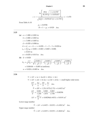
(a) d = U[0.748, 0.751]
µd =
0.751 + 0.748
2
= 0.7495 in
ˆσd =
0.751 − 0.748
2
√
3
= 0.000 866 in
f (x) =
1
b − a
=
1
0.751 − 0.748
= 333.3 in−1
F(x) =
x − 0.748
0.751 − 0.748
= 333.3(x − 0.748)
x1
f(x)
x
x2
␣ ␤
shi20396_ch02.qxd 7/21/03 3:28 PM Page 19

20. 20 Solutions Manual • Instructor’s Solution Manual to Accompany Mechanical Engineering Design
(b) F(x1) = F(0.748) = 0
F(x2) = (0.750 − 0.748)333.3 = 0.6667
If g(x) is truncated, PDF becomes
g(x) =
f (x)
F(x2) − F(x1)
=
333.3
0.6667 − 0
= 500 in−1
µx =
a + b
2
=
0.748 + 0.750
2
= 0.749 in
ˆσx =
b − a
2
√
3
=
0.750 − 0.748
2
√
3
= 0.000 577 in
2-18 From Table A-10, 8.1% corresponds to z1 = −1.4 and 5.5% corresponds to z2 = +1.6.
k1 = µ + z1 ˆσ
k2 = µ + z2 ˆσ
From which
µ =
z2k1 − z1k2
z2 − z1
=
1.6(9) − (−1.4)11
1.6 − (−1.4)
= 9.933
ˆσ =
k2 − k1
z2 − z1
=
11 − 9
1.6 − (−1.4)
= 0.6667
The original density function is
f (k) =
1
0.6667
√
2π
exp −
1
2
k − 9.933
0.6667
2
Ans.
2-19 From Prob. 2-1, µ = 122.9 kcycles and ˆσ = 30.3 kcycles.
z10 =
x10 − µ
ˆσ
=
x10 − 122.9
30.3
x10 = 122.9 + 30.3z10
From Table A-10, for 10 percent failure, z10 = −1.282
x10 = 122.9 + 30.3(−1.282)
= 84.1 kcycles Ans.
0.748
g(x) ϭ 500
x
f(x) ϭ 333.3
0.749 0.750 0.751
shi20396_ch02.qxd 7/21/03 3:28 PM Page 20

21. Chapter 2 21
2-20
x f fx f x2
x f/(Nw) f(x)
60 2 120 7200 60 0.002899 0.000399
70 1 70 4900 70 0.001449 0.001206
80 3 240 19200 80 0.004348 0.003009
90 5 450 40500 90 0.007246 0.006204
100 8 800 80000 100 0.011594 0.010567
110 12 1320 145200 110 0.017391 0.014871
120 6 720 86400 120 0.008696 0.017292
130 10 1300 169000 130 0.014493 0.016612
140 8 1120 156800 140 0.011594 0.013185
150 5 750 112500 150 0.007246 0.008647
160 2 320 51200 160 0.002899 0.004685
170 3 510 86700 170 0.004348 0.002097
180 2 360 64800 180 0.002899 0.000776
190 1 190 36100 190 0.001449 0.000237
200 0 0 0 200 0 5.98E-05
210 1 210 44100 210 0.001449 1.25E-05
69 8480
¯x = 122.8986 sx = 22.88719
x f/(Nw) f(x) x f/(Nw) f(x)
55 0 0.000214 145 0.011594 0.010935
55 0.002899 0.000214 145 0.007246 0.010935
65 0.002899 0.000711 155 0.007246 0.006518
65 0.001449 0.000711 155 0.002899 0.006518
75 0.001449 0.001951 165 0.002899 0.00321
75 0.004348 0.001951 165 0.004348 0.00321
85 0.004348 0.004425 175 0.004348 0.001306
85 0.007246 0.004425 175 0.002899 0.001306
95 0.007246 0.008292 185 0.002899 0.000439
95 0.011594 0.008292 185 0.001449 0.000439
105 0.011594 0.012839 195 0.001449 0.000122
105 0.017391 0.012839 195 0 0.000122
115 0.017391 0.016423 205 0 2.8E-05
115 0.008696 0.016423 205 0.001499 2.8E-05
125 0.008696 0.017357 215 0.001499 5.31E-06
125 0.014493 0.017357 215 0 5.31E-06
135 0.014493 0.015157
135 0.011594 0.015157
shi20396_ch02.qxd 7/21/03 3:28 PM Page 21

22. 22 Solutions Manual • Instructor’s Solution Manual to Accompany Mechanical Engineering Design
2-21
x f fx f x2
f/(Nw) f (x)
174 6 1044 181656 0.003807 0.001642
182 9 1638 298116 0.005711 0.009485
190 44 8360 1588400 0.027919 0.027742
198 67 13266 2626668 0.042513 0.041068
206 53 10918 2249108 0.033629 0.030773
214 12 2568 549552 0.007614 0.011671
222 6 1332 295704 0.003807 0.002241
1386 197 39126 7789204
¯x = 198.6091 sx = 9.695071
x f/(Nw) f (x)
170 0 0.000529
170 0.003807 0.000529
178 0.003807 0.004297
178 0.005711 0.004297
186 0.005711 0.017663
186 0.027919 0.017663
194 0.027919 0.036752
194 0.042513 0.036752
202 0.042513 0.038708
202 0.033629 0.038708
210 0.033629 0.020635
210 0.007614 0.020635
218 0.007614 0.005568
218 0.003807 0.005568
226 0.003807 0.00076
226 0 0.00076
Data
PDF
0
0.005
0.01
0.015
0.02
0.025
0.03
0.035
0.04
0.045
150 170 190 210
x
230
f
Histogram
PDF
0
0.002
0.004
0.006
0.008
0.01
0.012
0.014
0.016
0.018
f
x
0.02
0 50 100 150 200 250
shi20396_ch02.qxd 7/21/03 3:28 PM Page 22

23. Chapter 2 23
2-22
x f fx f x2
f/(Nw) f(x)
64 2 128 8192 0.008621 0.00548
68 6 408 27744 0.025862 0.017299
72 6 432 31104 0.025862 0.037705
76 9 684 51984 0.038793 0.056742
80 19 1520 121600 0.081897 0.058959
84 10 840 70560 0.043103 0.042298
88 4 352 30976 0.017241 0.020952
92 2 184 16928 0.008621 0.007165
624 58 4548 359088
¯x = 78.41379 sx = 6.572229
x f/(Nw) f(x) x f/(Nw) f(x)
62 0 0.002684 82 0.081897 0.052305
62 0.008621 0.002684 82 0.043103 0.052305
66 0.008621 0.010197 86 0.043103 0.03118
66 0.025862 0.010197 86 0.017241 0.03118
70 0.025862 0.026749 90 0.017241 0.012833
70 0.025862 0.026749 90 0.008621 0.012833
74 0.025862 0.048446 94 0.008621 0.003647
74 0.038793 0.048446 94 0 0.003647
78 0.038793 0.060581
78 0.081897 0.060581
2-23
¯σ =
4 ¯P
πd2
=
4(40)
π(12)
= 50.93 kpsi
ˆσσ =
4 ˆσP
πd2
=
4(8.5)
π(12)
= 10.82 kpsi
ˆσsy
= 5.9 kpsi
Data
PDF
x0
0.01
0.02
0.03
0.04
0.05
0.06
0.07
0.08
0.09
60 70 80 90 100
f
shi20396_ch02.qxd 7/21/03 3:28 PM Page 23

24. 24 Solutions Manual • Instructor’s Solution Manual to Accompany Mechanical Engineering Design
For no yield, m = Sy − σ ≥ 0
z =
m − µm
ˆσm
=
0 − µm
ˆσm
= −
µm
ˆσm
µm = ¯Sy − ¯σ = 27.47 kpsi,
ˆσm = ˆσ2
σ + ˆσ2
Sy
1/2
= 12.32 kpsi
z =
−27.47
12.32
= −2.230
From Table A-10, pf = 0.0129
R = 1 − pf = 1 − 0.0129 = 0.987 Ans.
2-24 For a lognormal distribution,
Eq. (2-18) µy = ln µx − ln 1 + C2
x
Eq. (2-19) ˆσy = ln 1 + C2
x
From Prob. (2-23)
µm = ¯Sy − ¯σ = µx
µy = ln ¯Sy − ln 1 + C2
Sy
− ln ¯σ − ln 1 + C2
σ
= ln
¯Sy
¯σ
1 + C2
σ
1 + C2
Sy
ˆσy = ln 1 + C2
Sy
+ ln 1 + C2
σ
1/2
= ln 1 + C2
Sy
1 + C2
σ
z = −
µ
ˆσ
= −
ln
¯Sy
¯σ
1 + C2
σ
1 + C2
Sy
ln 1 + C2
Sy
1 + C2
σ
¯σ =
4 ¯P
πd2
=
4(30)
π(12)
= 38.197 kpsi
ˆσσ =
4 ˆσP
πd2
=
4(5.1)
π(12)
= 6.494 kpsi
Cσ =
6.494
38.197
= 0.1700
CSy
=
3.81
49.6
= 0.076 81
0
m
shi20396_ch02.qxd 7/21/03 3:28 PM Page 24

25. Chapter 2 25
z = −
ln

 49.6
38.197
1 + 0.1702
1 + 0.076 812


ln (1 + 0.076 812)(1 + 0.1702)
= −1.470
From Table A-10
pf = 0.0708
R = 1 − pf = 0.929 Ans.
2-25
(a) a = 1.000 ± 0.001 in
b = 2.000 ± 0.003 in
c = 3.000 ± 0.005 in
d = 6.020 ± 0.006 in
¯w = d − a − b − c = 6.020 − 1 − 2 − 3 = 0.020 in
tw = tall = 0.001 + 0.003 + 0.005 + 0.006
= 0.015 in
w = 0.020 ± 0.015 in Ans.
(b) ¯w = 0.020
ˆσw = ˆσ2
all =
0.001
√
3
2
+
0.003
√
3
2
+
0.005
√
3
2
+
0.006
√
3
2
= 0.004 86 → 0.005 in (uniform)
w = 0.020 ± 0.005 in Ans.
2-26
V + V = (a + a)(b + b)(c + c)
V + V = abc + bc a + ac b + ab c + small higher order terms
V
¯V
.
=
a
a
+
b
b
+
c
c
Ans.
¯V = ¯a ¯b¯c = 1.25(1.875)(2.75) = 6.4453 in3
V
¯V
=
0.001
1.250
+
0.002
1.875
+
0.003
2.750
= 0.00296
V =
V
¯V
¯V = 0.00296(6.4453) = 0.0191 in3
Lower range number:
¯V − V = 6.4453 − 0.0191 = 6.4262 in3
Ans.
Upper range number:
¯V + V = 6.4453 + 0.0191 = 6.4644 in3
Ans.
shi20396_ch02.qxd 7/21/03 3:28 PM Page 25

26. 26 Solutions Manual • Instructor’s Solution Manual to Accompany Mechanical Engineering Design
2-27
(a)
wmax = 0.014 in, wmin = 0.004 in
¯w = (0.014 + 0.004)/2 = 0.009 in
w = 0.009 ± 0.005 in
¯w = ¯x − ¯y = ¯a − ¯b − ¯c
0.009 = ¯a − 0.042 − 1.000
¯a = 1.051 in
tw = tall
0.005 = ta + 0.002 + 0.002
ta = 0.005 − 0.002 − 0.002 = 0.001 in
a = 1.051 ± 0.001 in Ans.
(b) ˆσw = ˆσ2
all = ˆσ2
a + ˆσ2
b + ˆσ2
c
ˆσ2
a = ˆσ2
w − ˆσ2
b − ˆσ2
c
=
0.005
√
3
2
−
0.002
√
3
2
−
0.002
√
3
2
ˆσ2
a = 5.667(10−6
)
ˆσa = 5.667(10−6) = 0.00238 in
¯a = 1.051 in, ˆσa = 0.00238 in Ans.
2-28 Choose 15 mm as basic size, D, d. Table 2-8: fit is designated as 15H7/h6. From
Table A-11, the tolerance grades are D = 0.018 mm and d = 0.011 mm.
Hole: Eq. (2-38)
Dmax = D + D = 15 + 0.018 = 15.018 mm Ans.
Dmin = D = 15.000 mm Ans.
Shaft: From Table A-12, fundamental deviation δF = 0. From Eq. (2-39)
dmax = d + δF = 15.000 + 0 = 15.000 mm Ans.
dmin = d + δR − d = 15.000 + 0 − 0.011 = 14.989 mm Ans.
2-29 Choose 45 mm as basic size. Table 2-8 designates fit as 45H7/s6. From Table A-11, the
tolerance grades are D = 0.025 mm and d = 0.016 mm
Hole: Eq. (2-38)
Dmax = D + D = 45.000 + 0.025 = 45.025 mm Ans.
Dmin = D = 45.000 mm Ans.
a
c b
w
shi20396_ch02.qxd 7/21/03 3:28 PM Page 26

27. Chapter 2 27
Shaft: From Table A-12, fundamental deviation δF = +0.043 mm. From Eq. (2-40)
dmin = d + δF = 45.000 + 0.043 = 45.043 mm Ans.
dmax = d + δF + d = 45.000 + 0.043 + 0.016 = 45.059 mm Ans.
2-30 Choose 50 mm as basic size. From Table 2-8 fit is 50H7/g6. From Table A-11, the tolerance
grades are D = 0.025 mm and d = 0.016 mm.
Hole:
Dmax = D + D = 50 + 0.025 = 50.025 mm Ans.
Dmin = D = 50.000 mm Ans.
Shaft: From Table A-12 fundamental deviation = −0.009 mm
dmax = d + δF = 50.000 + (−0.009) = 49.991 mm Ans.
dmin = d + δF − d
= 50.000 + (−0.009) − 0.016
= 49.975 mm
2-31 Choose the basic size as 1.000 in. From Table 2-8, for 1.0 in, the fit is H8/f7. From
Table A-13, the tolerance grades are D = 0.0013 in and d = 0.0008 in.
Hole:
Dmax = D + ( D)hole = 1.000 + 0.0013 = 1.0013 in Ans.
Dmin = D = 1.0000 in Ans.
Shaft: From Table A-14: Fundamental deviation = −0.0008 in
dmax = d + δF = 1.0000 + (−0.0008) = 0.9992 in Ans.
dmin = d + δF − d = 1.0000 + (−0.0008) − 0.0008 = 0.9984 in Ans.
Alternatively,
dmin = dmax − d = 0.9992 − 0.0008 = 0.9984 in. Ans.
2-32
Do = W + Di + W
¯Do = ¯W + ¯Di + ¯W
= 0.139 + 3.734 + 0.139 = 4.012 in
tDo
= tall = 0.004 + 0.028 + 0.004
= 0.036 in
Do = 4.012 ± 0.036 in Ans.
Do
WDiW
shi20396_ch02.qxd 7/21/03 3:28 PM Page 27

28. 28 Solutions Manual • Instructor’s Solution Manual to Accompany Mechanical Engineering Design
2-33
Do = Di + 2W
¯Do = ¯Di + 2 ¯W = 208.92 + 2(5.33)
= 219.58 mm
tDo
=
all
t = tDi
+ 2tw
= 1.30 + 2(0.13) = 1.56 mm
Do = 219.58 ± 1.56 mm Ans.
2-34
Do = Di + 2W
¯Do = ¯Di + 2 ¯W = 3.734 + 2(0.139)
= 4.012 mm
tDo
=
all
t2 = t2
Do
+ (2 tw)2 1/2
= [0.0282
+ (2)2
(0.004)2
]1/2
= 0.029 in
Do = 4.012 ± 0.029 in Ans.
2-35
Do = Di + 2W
¯Do = ¯Di + 2 ¯W = 208.92 + 2(5.33)
= 219.58 mm
tDo
=
all
t2 = [1.302
+ (2)2
(0.13)2
]1/2
= 1.33 mm
Do = 219.58 ± 1.33 mm Ans.
2-36
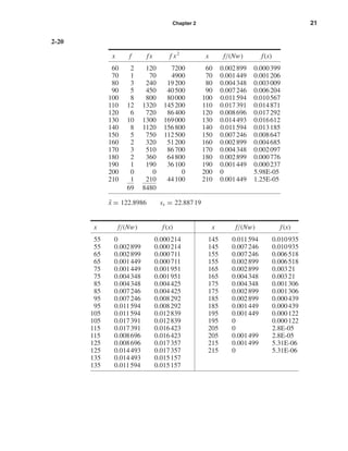
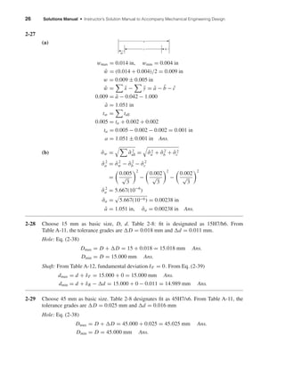
(a) w = F − W
¯w = ¯F − ¯W = 0.106 − 0.139
= −0.033 in
tw =
all
t = 0.003 + 0.004
tw = 0.007 in
wmax = ¯w + tw = −0.033 + 0.007 = −0.026 in
wmin = ¯w − tw = −0.033 − 0.007 = −0.040 in
The minimum “squeeze” is 0.026 in. Ans.
w
W
F
shi20396_ch02.qxd 7/21/03 3:28 PM Page 28

29. Chapter 2 29
(b)
Y = 3.992 ± 0.020 in
Do + w − Y = 0
w = Y − ¯Do
¯w = ¯Y − ¯Do = 3.992 − 4.012 = −0.020 in
tw =
all
t = tY + tDo
= 0.020 + 0.036 = 0.056 in
w = −0.020 ± 0.056 in
wmax = 0.036 in
wmin = −0.076 in
O-ring is more likely compressed than free prior to assembly of the
end plate.
2-37
(a) Figure defines w as gap.
The O-ring is “squeezed” at least 0.75 mm.
(b)
From the figure, the stochastic equation is:
Do + w = Y
or, w = Y − Do
¯w = ¯Y − ¯Do = 218.48 − 219.58 = −1.10 mm
tw =
all
t = tY + tDo
= 1.10 + 0.34 = 1.44 mm
wmax = ¯w + tw = −1.10 + 1.44 = 0.34 mm
wmin = ¯w − tw = −1.10 − 1.44 = −2.54 mm
The O-ring is more likely to be circumferentially compressed than free prior to as-
sembly of the end plate.
Ymax = ¯Do = 219.58 mm
Ymin = max[0.99 ¯Do, ¯Do − 1.52]
= max[0.99(219.58, 219.58 − 1.52)]
= 217.38 mm
Y = 218.48 ± 1.10 mm
Y
Do
w
w = F − W
¯w = ¯F − ¯W
= 4.32 − 5.33 = −1.01 mm
tw =
all
t = tF + tW = 0.13 + 0.13 = 0.26 mm
wmax = ¯w + tw = −1.01 + 0.26 = −0.75 mm
wmin = ¯w − tw = −1.01 − 0.26 = −1.27 mm
w
W
F
Ymax = ¯Do = 4.012 in
Ymin = max[0.99 ¯Do, ¯Do − 0.06]
= max[3.9719, 3.952] = 3.972 in
Y
Do
w
shi20396_ch02.qxd 8/6/03 11:07 AM Page 29

30. 30 Solutions Manual • Instructor’s Solution Manual to Accompany Mechanical Engineering Design
2-38
wmax = −0.020 in, wmin = −0.040 in
¯w =
1
2
(−0.020 + (−0.040)) = −0.030 in
tw =
1
2
(−0.020 − (−0.040)) = 0.010 in
b = 0.750 ± 0.001 in
c = 0.120 ± 0.005 in
d = 0.875 ± 0.001 in
¯w = ¯a − ¯b − ¯c − ¯d
−0.030 = ¯a − 0.875 − 0.120 − 0.750
¯a = 0.875 + 0.120 + 0.750 − 0.030
¯a = 1.715 in
Absolute:
tw =
all
t = 0.010 = ta + 0.001 + 0.005 + 0.001
ta = 0.010 − 0.001 − 0.005 − 0.001
= 0.003 in
a = 1.715 ± 0.003 in Ans.
Statistical: For a normal distribution of dimensions
t2
w =
all
t2
= t2
a + t2
b + t2
c + t2
d
ta = t2
w − t2
b − t2
c − t2
d
1/2
= (0.0102
− 0.0012
− 0.0052
− 0.0012
)1/2
= 0.0085
a = 1.715 ± 0.0085 in Ans.
2-39
x n nx nx2
93 19 1767 164 311
95 25 2375 225 625
97 38 3685 357 542
99 17 1683 166 617
101 12 1212 122 412
103 10 1030 106 090
105 5 525 55 125
107 4 428 45 796
109 4 436 47 524
111 2 222 24 624
136 13364 1315 704
¯x = 13 364/136 = 98.26 kpsi
sx =
1 315 704 − 13 3642
/136
135
1/2
= 4.30 kpsi
b c
w
d
a
shi20396_ch02.qxd 7/21/03 3:28 PM Page 30

31. Chapter 2 31
Under normal hypothesis,
z0.01 = (x0.01 − 98.26)/4.30
x0.01 = 98.26 + 4.30z0.01
= 98.26 + 4.30(−2.3267)
= 88.26
.
= 88.3 kpsi Ans.
2-40 From Prob. 2-39, µx = 98.26 kpsi, and ˆσx = 4.30 kpsi.
Cx = ˆσx/µx = 4.30/98.26 = 0.043 76
From Eqs. (2-18) and (2-19),
µy = ln(98.26) − 0.043 762
/2 = 4.587
ˆσy = ln(1 + 0.043 762) = 0.043 74
For a yield strength exceeded by 99% of the population,
z0.01 = (ln x0.01 − µy)/ˆσy ⇒ ln x0.01 = µy + ˆσyz0.01
From Table A-10, for 1% failure, z0.01 = −2.326. Thus,
ln x0.01 = 4.587 + 0.043 74(−2.326) = 4.485
x0.01 = 88.7 kpsi Ans.
The normal PDF is given by Eq. (2-14) as
f (x) =
1
4.30
√
2π
exp −
1
2
x − 98.26
4.30
2
For the lognormal distribution, from Eq. (2-17), defining g(x),
g(x) =
1
x(0.043 74)
√
2π
exp −
1
2
ln x − 4.587
0.043 74
2
x (kpsi) f/(Nw) f (x) g(x) x (kpsi) f/(Nw) f (x) g(x)
92 0.00000 0.03215 0.03263 102 0.03676 0.06356 0.06134
92 0.06985 0.03215 0.03263 104 0.03676 0.03806 0.03708
94 0.06985 0.05680 0.05890 104 0.01838 0.03806 0.03708
94 0.09191 0.05680 0.05890 106 0.01838 0.01836 0.01869
96 0.09191 0.08081 0.08308 106 0.01471 0.01836 0.01869
96 0.13971 0.08081 0.08308 108 0.01471 0.00713 0.00793
98 0.13971 0.09261 0.09297 108 0.01471 0.00713 0.00793
98 0.06250 0.09261 0.09297 110 0.01471 0.00223 0.00286
100 0.06250 0.08548 0.08367 110 0.00735 0.00223 0.00286
100 0.04412 0.08548 0.08367 112 0.00735 0.00056 0.00089
102 0.04412 0.06356 0.06134 112 0.00000 0.00056 0.00089
Note: rows are repeated to draw histogram
shi20396_ch02.qxd 7/21/03 3:28 PM Page 31

32. 32 Solutions Manual • Instructor’s Solution Manual to Accompany Mechanical Engineering Design
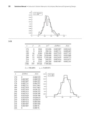
The normal and lognormal are almost the same. However the data is quite skewed and
perhaps a Weibull distribution should be explored. For a method of establishing the
Weibull parameters see Shigley, J. E., and C. R. Mischke, Mechanical Engineering Design,
McGraw-Hill, 5th ed., 1989, Sec. 4-12.
2-41 Let x = (S fe)104
x0 = 79 kpsi, θ = 86.2 kpsi, b = 2.6
Eq. (2-28)
¯x = x0 + (θ − x0) (1 + 1/b)
¯x = 79 + (86.2 − 79) (1 + 1/2.6)
= 79 + 7.2 (1.38)
From Table A-34, (1.38) = 0.88854
¯x = 79 + 7.2(0.888 54) = 85.4 kpsi Ans.
Eq. (2-29)
ˆσx = (θ − x0)[ (1 + 2/b) − 2
(1 + 1/b)]1/2
= (86.2 − 79)[ (1 + 2/2.6) − 2
(1 + 1/2.6)]1/2
= 7.2[0.923 76 − 0.888 542
]1/2
= 2.64 kpsi Ans.
Cx =
ˆσx
¯x
=
2.64
85.4
= 0.031 Ans.
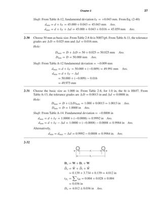
2-42
x = Sut
x0 = 27.7, θ = 46.2, b = 4.38
µx = 27.7 + (46.2 − 27.7) (1 + 1/4.38)
= 27.7 + 18.5 (1.23)
= 27.7 + 18.5(0.910 75)
= 44.55 kpsi Ans.
f(x)
g(x)
Histogram
0
0.02
0.04
0.06
0.08
0.1
0.12
0.14
0.16
90 92 94 96 98 100 102 104 106 108
x (kpsi)
Probabilitydensity
110 112
shi20396_ch02.qxd 7/21/03 3:28 PM Page 32

33. Chapter 2 33
ˆσx = (46.2 − 27.7)[ (1 + 2/4.38) − 2
(1 + 1/4.38)]1/2
= 18.5[ (1.46) − 2
(1.23)]1/2
= 18.5[0.8856 − 0.910 752
]1/2
= 4.38 kpsi Ans.
Cx =
4.38
44.55
= 0.098 Ans.
From the Weibull survival equation
R = exp −
x − x0
θ − x0
b
= 1 − p
R40 = exp −
x40 − x0
θ − x0
b
= 1 − p40
= exp −
40 − 27.7
46.2 − 27.7
4.38
= 0.846
p40 = 1 − R40 = 1 − 0.846 = 0.154 = 15.4% Ans.
2-43
x = Sut
x0 = 151.9, θ = 193.6, b = 8
µx = 151.9 + (193.6 − 151.9) (1 + 1/8)
= 151.9 + 41.7 (1.125)
= 151.9 + 41.7(0.941 76)
= 191.2 kpsi Ans.
ˆσx = (193.6 − 151.9)[ (1 + 2/8) − 2
(1 + 1/8)]1/2
= 41.7[ (1.25) − 2
(1.125)]1/2
= 41.7[0.906 40 − 0.941 762
]1/2
= 5.82 kpsi Ans.
Cx =
5.82
191.2
= 0.030
2-44
x = Sut
x0 = 47.6, θ = 125.6, b = 11.84
¯x = 47.6 + (125.6 − 47.6) (1 + 1/11.84)
¯x = 47.6 + 78 (1.08)
= 47.6 + 78(0.959 73) = 122.5 kpsi
ˆσx = (125.6 − 47.6)[ (1 + 2/11.84) − 2
(1 + 1/11.84)]1/2
= 78[ (1.08) − 2
(1.17)]1/2
= 78(0.959 73 − 0.936 702
)1/2
= 22.4 kpsi
shi20396_ch02.qxd 7/21/03 3:28 PM Page 33

34. 34 Solutions Manual • Instructor’s Solution Manual to Accompany Mechanical Engineering Design
From Prob. 2-42
p = 1 − exp −
x − x0
θ − θ0
b
= 1 − exp −
100 − 47.6
125.6 − 47.6
11.84
= 0.0090 Ans.
y = Sy
y0 = 64.1, θ = 81.0, b = 3.77
¯y = 64.1 + (81.0 − 64.1) (1 + 1/3.77)
= 64.1 + 16.9 (1.27)
= 64.1 + 16.9(0.902 50)
= 79.35 kpsi
σy = (81 − 64.1)[ (1 + 2/3.77) − (1 + 1/3.77)]1/2
σy = 16.9[(0.887 57) − 0.902 502
]1/2
= 4.57 kpsi
p = 1 − exp −
y − y0
θ − y0
3.77
p = 1 − exp −
70 − 64.1
81 − 64.1
3.77
= 0.019 Ans.
2-45 x = Sut = W[122.3, 134.6, 3.64] kpsi, p(x > 120) = 1 = 100% since x0 > 120 kpsi
p(x > 133) = exp −
133 − 122.3
134.6 − 122.3
3.64
= 0.548 = 54.8% Ans.
2-46 Using Eqs. (2-28) and (2-29) and Table A-34,
µn = n0 + (θ − n0) (1 + 1/b) = 36.9 + (133.6 − 36.9) (1 + 1/2.66) = 122.85 kcycles
ˆσn = (θ − n0)[ (1 + 2/b) − 2
(1 + 1/b)] = 34.79 kcycles
For the Weibull density function, Eq. (2-27),
fW (n) =
2.66
133.6 − 36.9
n − 36.9
133.6 − 36.9
2.66−1
exp −
n − 36.9
133.6 − 36.9
2.66
For the lognormal distribution, Eqs. (2-18) and (2-19) give,
µy = ln(122.85) − (34.79/122.85)2
/2 = 4.771
ˆσy = [1 + (34.79/122.85)2] = 0.2778
shi20396_ch02.qxd 7/21/03 3:28 PM Page 34

35. Chapter 2 35
From Eq. (2-17), the lognormal PDF is
fLN (n) =
1
0.2778 n
√
2π
exp −
1
2
ln n − 4.771
0.2778
2
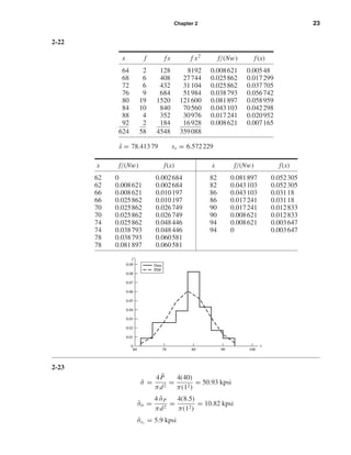
We form a table of densities fW (n) and fLN (n) and plot.
n(kcycles) fW (n) fLN (n)
40 9.1E-05 1.82E-05
50 0.000991 0.000241
60 0.002498 0.001233
70 0.004380 0.003501
80 0.006401 0.006739
90 0.008301 0.009913
100 0.009822 0.012022
110 0.010750 0.012644
120 0.010965 0.011947
130 0.010459 0.010399
140 0.009346 0.008492
150 0.007827 0.006597
160 0.006139 0.004926
170 0.004507 0.003564
180 0.003092 0.002515
190 0.001979 0.001739
200 0.001180 0.001184
210 0.000654 0.000795
220 0.000336 0.000529
The Weibull L10 life comes from Eq. (2-26) with a reliability of R = 0.90. Thus,
n0.10 = 36.9 + (133 − 36.9)[ln(1/0.90)]1/2.66
= 78.1 kcycles Ans.
f(n)
n, kcycles
0
0.004
0.002
0.006
0.008
0.010
0.012
0.014
0 10050 150 200
LN
W
250
shi20396_ch02.qxd 7/21/03 3:28 PM Page 35

36. 36 Solutions Manual • Instructor’s Solution Manual to Accompany Mechanical Engineering Design
The lognormal L10 life comes from the definition of the z variable. That is,
ln n0 = µy + ˆσyz or n0 = exp(µy + ˆσyz)
From Table A-10, for R = 0.90, z = −1.282. Thus,
n0 = exp[4.771 + 0.2778(−1.282)] = 82.7 kcycles Ans.
2-47 Form a table
x g(x)
i L(10−5
) fi fi x(10−5
) fi x2
(10−10
) (105
)
1 3.05 3 9.15 27.9075 0.0557
2 3.55 7 24.85 88.2175 0.1474
3 4.05 11 44.55 180.4275 0.2514
4 4.55 16 72.80 331.24 0.3168
5 5.05 21 106.05 535.5525 0.3216
6 5.55 13 72.15 400.4325 0.2789
7 6.05 13 78.65 475.8325 0.2151
8 6.55 6 39.30 257.415 0.1517
9 7.05 2 14.10 99.405 0.1000
10 7.55 0 0 0 0.0625
11 8.05 4 32.20 259.21 0.0375
12 8.55 3 25.65 219.3075 0.0218
13 9.05 0 0 0 0.0124
14 9.55 0 0 0 0.0069
15 10.05 1 10.05 101.0025 0.0038
100 529.50 2975.95
¯x = 529.5(105
)/100 = 5.295(105
) cycles Ans.
sx =
2975.95(1010
) − [529.5(105
)]2
/100
100 − 1
1/2
= 1.319(105
) cycles Ans.
Cx = s/¯x = 1.319/5.295 = 0.249
µy = ln 5.295(105
) − 0.2492
/2 = 13.149
ˆσy = ln(1 + 0.2492) = 0.245
g(x) =
1
x ˆσy
√
2π
exp −
1
2
ln x − µy
ˆσy
2
g(x) =
1.628
x
exp −
1
2
ln x − 13.149
0.245
2
shi20396_ch02.qxd 7/21/03 3:28 PM Page 36

37. Chapter 2 37
2-48
x = Su = W[70.3, 84.4, 2.01]
Eq. (2-28) µx = 70.3 + (84.4 − 70.3) (1 + 1/2.01)
= 70.3 + (84.4 − 70.3) (1.498)
= 70.3 + (84.4 − 70.3)0.886 17
= 82.8 kpsi Ans.
Eq. (2-29) ˆσx = (84.4 − 70.3)[ (1 + 2/2.01) − 2
(1 + 1/2.01)]1/2
ˆσx = 14.1[0.997 91 − 0.886 172
]1/2
= 6.502 kpsi
Cx =
6.502
82.8
= 0.079 Ans.
2-49 Take the Weibull equation for the standard deviation
ˆσx = (θ − x0)[ (1 + 2/b) − 2
(1 + 1/b)]1/2
and the mean equation solved for ¯x − x0
¯x − x0 = (θ − x0) (1 + 1/b)
Dividing the first by the second,
ˆσx
¯x − x0
=
[ (1 + 2/b) − 2
(1 + 1/b)]1/2
(1 + 1/b)
4.2
49 − 33.8
=
(1 + 2/b)
2(1 + 1/b)
− 1 =
√
R = 0.2763
0
0.1
0.2
0.3
0.4
0.5
105
g(x)
x, cycles
Superposed
histogram
and PDF
3.05(105
) 10.05(105
)
shi20396_ch02.qxd 7/21/03 3:28 PM Page 37

38. 38 Solutions Manual • Instructor’s Solution Manual to Accompany Mechanical Engineering Design
Make a table and solve for b iteratively
b
.
= 4.068 Using MathCad Ans.
θ = x0 +
¯x − x0
(1 + 1/b)
= 33.8 +
49 − 33.8
(1 + 1/4.068)
= 49.8 kpsi Ans.
2-50
x = Sy = W[34.7, 39, 2.93] kpsi
¯x = 34.7 + (39 − 34.7) (1 + 1/2.93)
= 34.7 + 4.3 (1.34)
= 34.7 + 4.3(0.892 22) = 38.5 kpsi
ˆσx = (39 − 34.7)[ (1 + 2/2.93) − 2
(1 + 1/2.93)]1/2
= 4.3[ (1.68) − 2
(1.34)]1/2
= 4.3[0.905 00 − 0.892 222
]1/2
= 1.42 kpsi Ans.
Cx = 1.42/38.5 = 0.037 Ans.
2-51
x (Mrev) f f x f x2
1 11 11 11
2 22 44 88
3 38 114 342
4 57 228 912
5 31 155 775
6 19 114 684
7 15 105 735
8 12 96 768
9 11 99 891
10 9 90 900
11 7 77 847
12 5 60 720
Sum 78 237 1193 7673
µx = 1193(106
)/237 = 5.034(106
) cycles
ˆσx =
7673(1012) − [1193(106)]2/237
237 − 1
= 2.658(106
) cycles
Cx = 2.658/5.034 = 0.528
b 1 + 2/b 1 + 1/b (1 + 2/b) (1 + 1/b)
3 1.67 1.33 0.90330 0.89338 0.363
4 1.5 1.25 0.88623 0.90640 0.280
4.1 1.49 1.24 0.88595 0.90852 0.271
shi20396_ch02.qxd 7/21/03 3:28 PM Page 38

39. Chapter 2 39
From Eqs. (2-18) and (2-19),
µy = ln[5.034(106
)] − 0.5282
/2 = 15.292
ˆσy = ln(1 + 0.5282) = 0.496
From Eq. (2-17), defining g(x),
g (x) =
1
x(0.496)
√
2π
exp −
1
2
ln x − 15.292
0.496
2
x(Mrev) f/(Nw) g(x) · (106
)
0.5 0.00000 0.00011
0.5 0.04641 0.00011
1.5 0.04641 0.05204
1.5 0.09283 0.05204
2.5 0.09283 0.16992
2.5 0.16034 0.16992
3.5 0.16034 0.20754
3.5 0.24051 0.20754
4.5 0.24051 0.17848
4.5 0.13080 0.17848
5.5 0.13080 0.13158
5.5 0.08017 0.13158
6.5 0.08017 0.09011
6.5 0.06329 0.09011
7.5 0.06329 0.05953
7.5 0.05063 0.05953
8.5 0.05063 0.03869
8.5 0.04641 0.03869
9.5 0.04641 0.02501
9.5 0.03797 0.02501
10.5 0.03797 0.01618
10.5 0.02954 0.01618
11.5 0.02954 0.01051
11.5 0.02110 0.01051
12.5 0.02110 0.00687
12.5 0.00000 0.00687
z =
ln x − µy
ˆσy
⇒ ln x = µy + ˆσyz = 15.292 + 0.496z
L10 life, where 10% of bearings fail, from Table A-10, z = −1.282. Thus,
ln x = 15.292 + 0.496(−1.282) = 14.66
∴ x = 2.32 × 106
rev Ans.
Histogram
PDF
x, Mrev
g(x)(106
)
0
0.05
0.1
0.15
0.2
0.25
0 2 4 6 8 10 12
shi20396_ch02.qxd 7/21/03 3:28 PM Page 39

40. 3-1 From Table A-20
Sut = 470 MPa (68 kpsi), Sy = 390 MPa (57 kpsi) Ans.
3-2 From Table A-20
Sut = 620 MPa (90 kpsi), Sy = 340 MPa (49.5 kpsi) Ans.
3-3 Comparison of yield strengths:
Sut of G10500 HR is
620
470
= 1.32 times larger than SAE1020 CD Ans.
Syt of SAE1020 CD is
390
340
= 1.15 times larger than G10500 HR Ans.
From Table A-20, the ductilities (reduction in areas) show,
SAE1020 CD is
40
35
= 1.14 times larger than G10500 Ans.
The stiffness values of these materials are identical Ans.
Table A-20 Table A-5
Sut Sy Ductility Stiffness
MPa (kpsi) MPa (kpsi) R% GPa (Mpsi)
SAE1020 CD 470(68) 390 (57) 40 207(30)
UNS10500 HR 620(90) 340(495) 35 207(30)
3-4 From Table A-21
1040 Q&T ¯Sy = 593 (86) MPa (kpsi) at 205◦
C (400◦
F) Ans.
3-5 From Table A-21
1040 Q&T R = 65% at 650◦
C (1200◦
F) Ans.
3-6 Using Table A-5, the specific strengths are:
UNS G10350 HR steel:
Sy
W
=
39.5(103
)
0.282
= 1.40(105
) in Ans.
2024 T4 aluminum:
Sy
W
=
43(103
)
0.098
= 4.39(105
) in Ans.
Ti-6Al-4V titanium:
Sy
W
=
140(103
)
0.16
= 8.75(105
) in Ans.
ASTM 30 gray cast iron has no yield strength. Ans.
Chapter 3
shi20396_ch03.qxd 8/18/03 10:18 AM Page 40

41. Chapter 3 41
3-7 The specific moduli are:
UNS G10350 HR steel:
E
W
=
30(106
)
0.282
= 1.06(108
) in Ans.
2024 T4 aluminum:
E
W
=
10.3(106
)
0.098
= 1.05(108
) in Ans.
Ti-6Al-4V titanium:
E
W
=
16.5(106
)
0.16
= 1.03(108
) in Ans.
Gray cast iron:
E
W
=
14.5(106
)
0.26
= 5.58(107
) in Ans.
3-8 2G(1 + ν) = E ⇒ ν =
E − 2G
2G
From Table A-5
Steel: ν =
30 − 2(11.5)
2(11.5)
= 0.304 Ans.
Aluminum: ν =
10.4 − 2(3.90)
2(3.90)
= 0.333 Ans.
Beryllium copper: ν =
18 − 2(7)
2(7)
= 0.286 Ans.
Gray cast iron: ν =
14.5 − 2(6)
2(6)
= 0.208 Ans.
3-9
0
10
0 0.002
0.1
0.004
0.2
0.006
0.3
0.008
0.4
0.010
0.5
0.012
0.6
0.014
0.7
0.016
0.8
(Lower curve)
(Upper curve)
20
30
40
50
StressP͞A0kpsi
Strain, ⑀
60
70
80
E
Y
U
Su ϭ 85.5 kpsi Ans.
E ϭ 90͞0.003 ϭ 30 000 kpsi Ans.
Sy ϭ 45.5 kpsi Ans.
R ϭ (100) ϭ 45.8% Ans.
A0 Ϫ AF
A0
ϭ
0.1987 Ϫ 0.1077
0.1987
⑀ ϭ
⌬l
l0
ϭ
l Ϫ l0
l0
l
l0
ϭ Ϫ 1
A
A0
ϭ Ϫ 1
shi20396_ch03.qxd 8/18/03 10:18 AM Page 41

42. 42 Solutions Manual • Instructor’s Solution Manual to Accompany Mechanical Engineering Design
3-10 To plot σtrue vs. ε, the following equations are applied to the data.
A0 =
π(0.503)2
4
= 0.1987 in2
Eq. (3-4) ε = ln
l
l0
for 0 ≤ L ≤ 0.0028 in
ε = ln
A0
A
for L > 0.0028 in
σtrue =
P
A
The results are summarized in the table below and plotted on the next page.
The last 5 points of data are used to plot log σ vs log ε
The curve fit gives m = 0.2306
log σ0 = 5.1852 ⇒ σ0 = 153.2 kpsi
Ans.
For 20% cold work, Eq. (3-10) and Eq. (3-13) give,
A = A0(1 − W) = 0.1987(1 − 0.2) = 0.1590 in2
ε = ln
A0
A
= ln
0.1987
0.1590
= 0.2231
Eq. (3-14):
Sy = σ0εm
= 153.2(0.2231)0.2306
= 108.4 kpsi Ans.
Eq. (3-15), with Su = 85.5 kpsi from Prob. 3-9,
Su =
Su
1 − W
=
85.5
1 − 0.2
= 106.9 kpsi Ans.
P L A ε σtrue log ε log σtrue
0 0 0.198713 0 0
1000 0.0004 0.198713 0.0002 5032.388 −3.69901 3.701774
2000 0.0006 0.198713 0.0003 10064.78 −3.52294 4.002804
3000 0.0010 0.198713 0.0005 15097.17 −3.30114 4.178895
4000 0.0013 0.198713 0.00065 20129.55 −3.18723 4.303834
7000 0.0023 0.198713 0.001149 35226.72 −2.93955 4.546872
8400 0.0028 0.198713 0.001399 42272.06 −2.85418 4.626053
8800 0.0036 0.1984 0.001575 44354.84 −2.80261 4.646941
9200 0.0089 0.1978 0.004604 46511.63 −2.33685 4.667562
9100 0.1963 0.012216 46357.62 −1.91305 4.666121
13200 0.1924 0.032284 68607.07 −1.49101 4.836369
15200 0.1875 0.058082 81066.67 −1.23596 4.908842
17000 0.1563 0.240083 108765.2 −0.61964 5.03649
16400 0.1307 0.418956 125478.2 −0.37783 5.098568
14800 0.1077 0.612511 137418.8 −0.21289 5.138046
shi20396_ch03.qxd 8/18/03 10:18 AM Page 42

43. Chapter 3 43
3-11 Tangent modulus at σ = 0 is
E0 =
σ
ε
.
=
5000 − 0
0.2(10−3) − 0
= 25(106
) psi
At σ = 20 kpsi
E20
.
=
(26 − 19)(103
)
(1.5 − 1)(10−3)
= 14.0(106
) psi Ans.
ε(10−3
) σ (kpsi)
0 0
0.20 5
0.44 10
0.80 16
1.0 19
1.5 26
2.0 32
2.8 40
3.4 46
4.0 49
5.0 54
3-12 From Prob. 2-8, for y = a1x + a2x2
a1 =
y x3
− xy x2
x x3 − ( x2)2
a2 =
x xy − y x2
x x3 − ( x2)2
log ␧
log␴
y ϭ 0.2306x ϩ 5.1852
4.8
4.9
5
5.1
5.2
Ϫ1.6 Ϫ1.4 Ϫ1.2 Ϫ1 Ϫ0.8 Ϫ0.6 Ϫ0.4 Ϫ0.2 0
␧true
␴true(psi)
0
20000
40000
60000
80000
100000
120000
140000
160000
0 0.1 0.2 0.3 0.4 0.5 0.6 0.7
␧ (10Ϫ3
)
(Sy)0.001 ϭ˙ 35 kpsi Ans.
␴(kpsi)
0
10
20
30
40
50
60
0 1 2 3 4 5
shi20396_ch03.qxd 8/18/03 10:18 AM Page 43

44. 44 Solutions Manual • Instructor’s Solution Manual to Accompany Mechanical Engineering Design
Let x represent ε(10−3
) and y represent σ (kpsi),
x y x2
x3
xy
0 0 0 0 0
0.2 5 0.04 0.008 1.0
0.44 10 0.1936 0.085184 4.4
0.80 16 0.64 0.512 12.8
1.0 19 1.00 1.000 19.0
1.5 26 2.25 3.375 39.0
2.0 32 4.00 8.000 64.0
2.8 40 7.84 21.952 112.0
3.4 46 11.56 39.304 156.4
4.0 49 16.00 64.000 196.0
5.0 54 25.00 125.000 270.0
= 21.14 297 68.5236 263.2362 874.6
Substituting,
a1 =
297(263.2362) − 874.6(68.5236)
21.14(263.2362) − (68.5236)2
= 20.993 67
a2 =
21.14(874.6) − 297(68.5236)
21.14(263.2362) − (68.5236)2
= −2.142 42
The tangent modulus is
dy
dx
=
dσ
dε
= 20.993 67 − 2(2.142 42)x = 20.993 67 − 4.284 83x
At σ = 0, E0 = 20.99 Mpsi Ans.
At σ = 20 kpsi
20 = 20.993 67x − 2.142 42x2
⇒ x = 1.069, 8.73
Taking the first root, ε = 1.069 and the tangent modulus is
E20 = 20.993 67 − 4.284 83(1.069) = 16.41 Mpsi Ans.
Determine the equation for the 0.1 percent offset line
y = 20.99x + b at y = 0, x = 1 ∴ b = −20.99
y = 20.99x − 20.99 = 20.993 67x − 2.142 42x2
2.142 42x2
− 20.99 = 0 ⇒ x = 3.130
(Sy)0.001 = 20.99(3.13) − 2.142(3.13)2
= 44.7 kpsi Ans.
3-13 Since |εo| = |εi |
ln
R + h
R + N
= ln
R
R + N
= −ln
R + N
R
R + h
R + N
=
R + N
R
(R + N)2
= R(R + h)
From which, N2
+ 2RN − Rh = 0
shi20396_ch03.qxd 8/18/03 10:18 AM Page 44

45. Chapter 3 45
The roots are: N = R −1 ± 1 +
h
R
1/2
The + sign being significant,
N = R 1 +
h
R
1/2
− 1 Ans.
Substitute for N in
εo = ln
R + h
R + N
Gives ε0 = ln





R + h
R + R 1 +
h
R
1/2
− R





= ln 1 +
h
R
1/2
Ans.
These constitute a useful pair of equations in cold-forming situations, allowing the surface
strains to be found so that cold-working strength enhancement can be estimated.
3-14
τ =
16T
πd3
=
16T
π(12.5)3
10−6
(10−3)3
= 2.6076T MPa
γ =
θ◦ π
180
r
L
=
θ◦ π
180
(12.5)
350
= 6.2333(10−4
)θ◦
For G, take the first 10 data points for the linear part of the curve.
θ γ (10−3
) τ (MPa)
T (deg.) γ (10−3
) τ (MPa) x y x2
xy
0 0 0 0 0 0 0 0
7.7 0.38 0.236865 20.07852 0.236865 20.07852 0.056105 4.7559
15.3 0.80 0.498664 39.89628 0.498664 39.89628 0.248666 19.8948
23.0 1.24 0.772929 59.9748 0.772929 59.9748 0.597420 46.3563
30.7 1.64 1.022261 80.05332 1.022261 80.05332 1.045018 81.8354
38.3 2.01 1.252893 99.87108 1.252893 99.87108 1.569742 125.1278
46.0 2.40 1.495992 119.9496 1.495992 119.9496 2.237992 179.4436
53.7 2.85 1.776491 140.0281 1.776491 140.0281 3.155918 248.7586
61.4 3.25 2.025823 160.1066 2.025823 160.1066 4.103957 324.3476
69.0 3.80 2.368654 179.9244 2.368654 179.9244 5.610522 426.1786
76.7 4.50 2.804985 200.0029 = 11.45057 899.8828 18.62534 1456.6986
80.0 5.10 3.178983 208.608
85.0 6.48 4.039178 221.646
90.0 8.01 4.992873 234.684
95.0 9.58 5.971501 247.722
100.0 11.18 6.968829 260.76
shi20396_ch03.qxd 8/18/03 10:18 AM Page 45

46. 46 Solutions Manual • Instructor’s Solution Manual to Accompany Mechanical Engineering Design
y = mx + b, τ = y, γ = x where m is the shear modulus G,
m =
N xy − x y
N x2 − ( x)2
= 77.3
MPa
10−3
= 77.3 GPa Ans.
b =
y − m x
N
= 1.462 MPa
From curve Sys
.
= 200 MPa Ans.
Note since τ is not uniform, the offset yield does not apply, so we are using the elastic
limit as an approximation.
3-15
x f f x f x2
38.5 2 77.0 2964.50
39.5 9 355.5 14042.25
40.5 30 1215.0 49207.50
41.5 65 2697.5 111946.30
42.5 101 4292.5 182431.30
43.5 112 4872.0 211932.00
44.5 90 4005.0 178222.50
45.5 54 2457.0 111793.50
46.5 25 1162.5 54056.25
47.5 9 427.5 20306.25
48.5 2 97.0 4704.50
49.5 1 49.5 2 450.25
= 528.0 500 21708.0 944057.00
¯x = 21 708/500 = 43.416, ˆσx =
944 057 − (21 7082/500)
500 − 1
= 1.7808
Cx = 1.7808/43.416 = 0.041 02,
¯y = ln 43.416 − ln(1 + 0.041 022
) = 3.7691
␥ (10Ϫ3
)
␶(MPa)
0
50
100
150
200
250
300
0 1 2 3 4 5 6 7
shi20396_ch03.qxd 8/18/03 10:18 AM Page 46

47. Chapter 3 47
ˆσy = ln(1 + 0.041 022) = 0.0410,
g(x) =
1
x(0.0410)
√
2π
exp −
1
2
ln x − 3.7691
0.0410
2
x f/(Nw) g(x) x f/(Nw) g(x)
38 0 0.001488 45 0.180 0.142268
38 0.004 0.001488 45 0.108 0.142268
39 0.004 0.009057 46 0.108 0.073814
39 0.018 0.009057 46 0.050 0.073814
40 0.018 0.035793 47 0.050 0.029410
40 0.060 0.035793 47 0.018 0.029410
41 0.060 0.094704 48 0.018 0.009152
41 0.130 0.094704 48 0.004 0.009152
42 0.130 0.172538 49 0.004 0.002259
42 0.202 0.172538 49 0.002 0.002259
43 0.202 0.222074 50 0.002 0.000449
43 0.224 0.222074 50 0 0.000449
44 0.224 0.206748
44 0.180 0.206748
Sy = LN(43.42, 1.781) kpsi Ans.
3-16 From Table A-22
AISI 1212 Sy = 28.0 kpsi, σf = 106 kpsi, Sut = 61.5 kpsi
σ0 = 110 kpsi, m = 0.24, εf = 0.85
From Eq. (3-12) εu = m = 0.24
Eq. (3-10)
A0
Ai
=
1
1 − W
=
1
1 − 0.2
= 1.25
Eq. (3-13) εi = ln 1.25 = 0.2231 ⇒ εi < εu
x
f(x)
0
0.05
0.1
0.15
0.2
0.25
35 40 45 50
Histogram
PDF
shi20396_ch03.qxd 8/18/03 10:18 AM Page 47

48. 48 Solutions Manual • Instructor’s Solution Manual to Accompany Mechanical Engineering Design
Eq. (3-14) Sy = σ0εm
i = 110(0.2231)0.24
= 76.7 kpsi Ans.
Eq. (3-15) Su =
Su
1 − W
=
61.5
1 − 0.2
= 76.9 kpsi Ans.
3-17 For HB = 250,
Eq. (3-17) Su = 0.495 (250) = 124 kpsi
= 3.41 (250) = 853 MPa
Ans.
3-18 For the data given,
HB = 2530 H2
B = 640 226
¯HB =
2530
10
= 253 ˆσH B =
640 226 − (2530)2/10
9
= 3.887
Eq. (3-17)
¯Su = 0.495(253) = 125.2 kpsi Ans.
¯σsu = 0.495(3.887) = 1.92 kpsi Ans.
3-19 From Prob. 3-18, ¯HB = 253 and ˆσHB = 3.887
Eq. (3-18)
¯Su = 0.23(253) − 12.5 = 45.7 kpsi Ans.
ˆσsu = 0.23(3.887) = 0.894 kpsi Ans.
3-20
(a) uR
.
=
45.52
2(30)
= 34.5 in · lbf/in3
Ans.
(b)
P L A A0/A − 1 ε σ = P/A0
0 0 0 0
1000 0.0004 0.0002 5032.39
2000 0.0006 0.0003 10064.78
3000 0.0010 0.0005 15097.17
4000 0.0013 0.00065 20129.55
7000 0.0023 0.00115 35226.72
8400 0.0028 0.0014 42272.06
8800 0.0036 0.0018 44285.02
9200 0.0089 0.00445 46297.97
9100 0.1963 0.012291 0.012291 45794.73
13200 0.1924 0.032811 0.032811 66427.53
15200 0.1875 0.059802 0.059802 76492.30
17000 0.1563 0.271355 0.271355 85550.60
16400 0.1307 0.520373 0.520373 82531.17
14800 0.1077 0.845059 0.845059 74479.35
shi20396_ch03.qxd 8/18/03 10:18 AM Page 48

49. Chapter 3 49
uT
.
=
5
i=1
Ai =
1
2
(43 000)(0.001 5) + 45 000(0.004 45 − 0.001 5)
+
1
2
(45 000 + 76 500)(0.059 8 − 0.004 45)
+81 000(0.4 − 0.059 8) + 80 000(0.845 − 0.4)
.
= 66.7(103
)in · lbf/in3
Ans.
␧
␴
0
20000
10000
30000
40000
50000
60000
70000
80000
90000
0 0.2 0.4 0.6 0.8
A3
A4 A5
Last 6 data points
First 9 data points
␧
␴
0
A1 A215000
10000
5000
20000
25000
30000
35000
40000
45000
50000
0 0.0020.001 0.003 0.004 0.005
␧
␴
0
20000
10000
30000
40000
50000
60000
70000
80000
90000
0 0.2 0.4
All data points
0.6 0.8
shi20396_ch03.qxd 8/18/03 10:18 AM Page 49

50. Chapter 4
4-1
1
RC
RA
RB
RD
C
A B
W
D
1
23
RB
RA
W
RB
RC
RA
2
1
W
RA
RBx
RBx RBy
RBy
RB
2
1
1
Scale of
corner magnified
W
A
B
(e)
(f)
(d)
W
A
RA RB
B
1
2
W
A
RA RB
B
11
2
(a) (b)
(c)
shi20396_ch04.qxd 8/18/03 10:35 AM Page 50

51. Chapter 4 51
4-2
(a) RA = 2 sin 60 = 1.732 kN Ans.
RB = 2 sin 30 = 1 kN Ans.
(b) S = 0.6 m
α = tan−1 0.6
0.4 + 0.6
= 30.96◦
RA
sin 135
=
800
sin 30.96
⇒ RA = 1100 N Ans.
RO
sin 14.04
=
800
sin 30.96
⇒ RO = 377 N Ans.
(c)
RO =
1.2
tan 30
= 2.078 kN Ans.
RA =
1.2
sin 30
= 2.4 kN Ans.
(d) Step 1: Find RA and RE
h =
4.5
tan 30
= 7.794 m
ۗ+ MA = 0
9RE − 7.794(400 cos 30) − 4.5(400 sin 30) = 0
RE = 400 N Ans.
Fx = 0 RAx + 400 cos 30 = 0 ⇒ RAx = −346.4 N
Fy = 0 RAy + 400 − 400 sin 30 = 0 ⇒ RAy = −200 N
RA = 346.42 + 2002 = 400 N Ans.
D
C
h
B
y
E xA
4.5 m
9 m
400 N
3
42
30°
60°
RAy
RA
RAx
RE
1.2 kN
60°
RA
RO
60°90°
30°
1.2 kN
RARO
45Њ Ϫ 30.96Њ ϭ 14.04Њ
135°
30.96°
30.96°
800 N
RA
RO
O
0.4 m
45°
800 N
␣
0.6 m
A
s
RA
RO
B
60°
90°
30°
2 kN
RA
RB
2
1
2 kN
60°30°
RA
RB
shi20396_ch04.qxd 8/18/03 10:35 AM Page 51

52. 52 Solutions Manual • Instructor’s Solution Manual to Accompany Mechanical Engineering Design
Step 2: Find components of RC on link 4 and RD
ۗ+ MC = 0
400(4.5) − (7.794 − 1.9)RD = 0 ⇒ RD = 305.4 N Ans.
Fx = 0 ⇒ (RCx)4 = 305.4 N
Fy = 0 ⇒ (RCy)4 = −400 N
Step 3: Find components of RC on link 2
Fx = 0
(RCx)2 + 305.4 − 346.4 = 0 ⇒ (RCx)2 = 41 N
Fy = 0
(RCy)2 = 200 N
4-3
(a)
ۗ+ M0 = 0
−18(60) + 14R2 + 8(30) − 4(40) = 0
R2 = 71.43 lbf
Fy = 0: R1 − 40 + 30 + 71.43 − 60 = 0
R1 = −1.43 lbf
M1 = −1.43(4) = −5.72 lbf · in
M2 = −5.72 − 41.43(4) = −171.44 lbf · in
M3 = −171.44 − 11.43(6) = −240 lbf · in
M4 = −240 + 60(4) = 0 checks!
4" 4" 6" 4"
Ϫ1.43
Ϫ41.43
Ϫ11.43
60
40 lbf 60 lbf
30 lbf
x
x
x
O
A B C D
y
R1 R2
M1
M2 M3
M4
O
V (lbf)
M
(lbf• in)
O
CC
DB
A
B D
E
305.4 N
346.4 N
305.4 N
41 N
400 N
200 N
400 N
200 N
400 N
Pin C
30°
305.4 N
400 N
400 N200 N
41 N
305.4 N
200 N
346.4 N
305.4 N
(RCx)2
(RCy)2
C
B
A
2
400 N
4
RD
(RCx)4
(RCy)4
D
C
E
Ans.
shi20396_ch04.qxd 8/18/03 10:35 AM Page 52

53. Chapter 4 53
(b) Fy = 0
R0 = 2 + 4(0.150) = 2.6kN
M0 = 0
M0 = 2000(0.2) + 4000(0.150)(0.425)
= 655 N · m
M1 = −655 + 2600(0.2) = −135 N · m
M2 = −135 + 600(0.150) = −45 N · m
M3 = −45 +
1
2
600(0.150) = 0 checks!
(c) M0 = 0: 10R2 − 6(1000) = 0 ⇒ R2 = 600 lbf
Fy = 0: R1 − 1000 + 600 = 0 ⇒ R1 = 400 lbf
M1 = 400(6) = 2400 lbf · ft
M2 = 2400 − 600(4) = 0 checks!
(d) ۗ+ MC = 0
−10R1 + 2(2000) + 8(1000) = 0
R1 = 1200 lbf
Fy = 0: 1200 − 1000 − 2000 + R2 = 0
R2 = 1800 lbf
M1 = 1200(2) = 2400 lbf · ft
M2 = 2400 + 200(6) = 3600 lbf · ft
M3 = 3600 − 1800(2) = 0 checks!
2000 lbf1000 lbf
R1
O
O
M1
M2
M3
R2
6 ft 2 ft2 ft
A B C
y
M
1200
Ϫ1800
200
x
x
x
6 ft 4 ft
A
O
O
O
B
Ϫ600
M1
M2
V (lbf)
1000 lbfy
R1 R2
400
M
(lbf•ft)
x
x
x
V (kN)
150 mm200 mm 150 mm
2.6
Ϫ655
M
(N•m)
0.6
M1
M2
M3
2 kN 4 kN/my
A
O
O
O
O
B C
RO
MO
x
x
x
shi20396_ch04.qxd 8/18/03 10:35 AM Page 53

54. 54 Solutions Manual • Instructor’s Solution Manual to Accompany Mechanical Engineering Design
(e) ۗ+ MB = 0
−7R1 + 3(400) − 3(800) = 0
R1 = −171.4 lbf
Fy = 0: −171.4 − 400 + R2 − 800 = 0
R2 = 1371.4 lbf
M1 = −171.4(4) = −685.7 lbf · ft
M2 = −685.7 − 571.4(3) = −2400 lbf · ft
M3 = −2400 + 800(3) = 0 checks!
(f) Break at A
R1 = VA =
1
2
40(8) = 160 lbf
ۗ + MD = 0
12(160) − 10R2 + 320(5) = 0
R2 = 352 lbf
Fy = 0
−160 + 352 − 320 + R3 = 0
R3 = 128 lbf
M1 =
1
2
160(4) = 320 lbf · in
M2 = 320 −
1
2
160(4) = 0 checks! (hinge)
M3 = 0 − 160(2) = −320 lbf · in
M4 = −320 + 192(5) = 640 lbf · in
M5 = 640 − 128(5) = 0 checks!
40 lbf/in
V (lbf)
O
O
160
Ϫ160
Ϫ128
192
M
320 lbf
160 lbf 352 lbf 128 lbf
M1
M2
M3
M4
M5
x
x
x
8"
5"
2"
5"
40 lbf/in
160 lbf
O
A
y
B D
C
A
320 lbf
R2 R3
R1 VA
A
O
O
O
C
M
V (lbf)
800
Ϫ171.4
Ϫ571.4
3 ft 3 ft4 ft
800 lbf400 lbf
B
y
M1
M2
M3
R1 R2
x
x
x
shi20396_ch04.qxd 8/18/03 10:35 AM Page 54

55. Chapter 4 55
4-4
(a) q = R1 x −1
− 40 x − 4 −1
+ 30 x − 8 −1
+ R2 x − 14 −1
− 60 x − 18 −1
V = R1 − 40 x − 4 0
+ 30 x − 8 0
+ R2 x − 14 0
− 60 x − 18 0
(1)
M = R1x − 40 x − 4 1
+ 30 x − 8 1
+ R2 x − 14 1
− 60 x − 18 1
(2)
for x = 18+
V = 0 and M = 0 Eqs. (1) and (2) give
0 = R1 − 40 + 30 + R2 − 60 ⇒ R1 + R2 = 70 (3)
0 = R1(18) − 40(14) + 30(10) + 4R2 ⇒ 9R1 + 2R2 = 130 (4)
Solve (3) and (4) simultaneously to get R1 = −1.43 lbf, R2 = 71.43 lbf. Ans.
From Eqs. (1) and (2), at x = 0+
, V = R1 = −1.43 lbf, M = 0
x = 4+
: V = −1.43 − 40 = −41.43, M = −1.43x
x = 8+
: V = −1.43 − 40 + 30 = −11.43
M = −1.43(8) − 40(8 − 4)1
= −171.44
x = 14+
: V = −1.43 − 40 + 30 + 71.43 = 60
M = −1.43(14) − 40(14 − 4) + 30(14 − 8) = −240.
x = 18+
: V = 0, M = 0 See curves of V and M in Prob. 4-3 solution.
(b) q = R0 x −1
− M0 x −2
− 2000 x − 0.2 −1
− 4000 x − 0.35 0
+ 4000 x − 0.5 0
V = R0 − M0 x −1
− 2000 x − 0.2 0
− 4000 x − 0.35 1
+ 4000 x − 0.5 1
(1)
M = R0x − M0 − 2000 x − 0.2 1
− 2000 x − 0.35 2
+ 2000 x − 0.5 2
(2)
at x = 0.5+
m, V = M = 0, Eqs. (1) and (2) give
R0 − 2000 − 4000(0.5 − 0.35) = 0 ⇒ R1 = 2600 N = 2.6 kN Ans.
R0(0.5) − M0 − 2000(0.5 − 0.2) − 2000(0.5 − 0.35)2
= 0
with R0 = 2600 N, M0 = 655 N · m Ans.
With R0 and M0, Eqs. (1) and (2) give the same V and M curves as Prob. 4-3 (note for
V, M0 x −1
has no physical meaning).
(c) q = R1 x −1
− 1000 x − 6 −1
+ R2 x − 10 −1
V = R1 − 1000 x − 6 0
+ R2 x − 10 0
(1)
M = R1x − 1000 x − 6 1
+ R2 x − 10 1
(2)
at x = 10+
ft, V = M = 0, Eqs. (1) and (2) give
R1 − 1000 + R2 = 0 ⇒ R1 + R2 = 1000
10R1 − 1000(10 − 6) = 0 ⇒ R1 = 400 lbf, R2 = 1000 − 400 = 600 lbf
0 ≤ x ≤ 6: V = 400 lbf, M = 400x
6 ≤ x ≤ 10: V = 400 − 1000(x − 6)0
= 600 lbf
M = 400x − 1000(x − 6) = 6000 − 600x
See curves of Prob. 4-3 solution.
shi20396_ch04.qxd 8/18/03 10:35 AM Page 55

56. 56 Solutions Manual • Instructor’s Solution Manual to Accompany Mechanical Engineering Design
(d) q = R1 x −1
− 1000 x − 2 −1
− 2000 x − 8 −1
+ R2 x − 10 −1
V = R1 − 1000 x − 2 0
− 2000 x − 8 0
+ R2 x − 10 0
(1)
M = R1x − 1000 x − 2 1
− 2000 x − 8 1
+ R2 x − 10 1
(2)
At x = 10+
, V = M = 0 from Eqs. (1) and (2)
R1 − 1000 − 2000 + R2 = 0 ⇒ R1 + R2 = 3000
10R1 − 1000(10 − 2) − 2000(10 − 8) = 0 ⇒ R1 = 1200 lbf,
R2 = 3000 − 1200 = 1800 lbf
0 ≤ x ≤ 2: V = 1200 lbf, M = 1200x lbf · ft
2 ≤ x ≤ 8: V = 1200 − 1000 = 200 lbf
M = 1200x − 1000(x − 2) = 200x + 2000 lbf · ft
8 ≤ x ≤ 10: V = 1200 − 1000 − 2000 = −1800 lbf
M = 1200x − 1000(x − 2) − 2000(x − 8) = −1800x + 18 000 lbf · ft
Plots are the same as in Prob. 4-3.
(e) q = R1 x −1
− 400 x − 4 −1
+ R2 x − 7 −1
− 800 x − 10 −1
V = R1 − 400 x − 4 0
+ R2 x − 7 0
− 800 x − 10 0
(1)
M = R1x − 400 x − 4 1
+ R2 x − 7 1
− 800 x − 10 1
(2)
at x = 10+
, V = M = 0
R1 − 400 + R2 − 800 = 0 ⇒ R1 + R2 = 1200 (3)
10R1 − 400(6) + R2(3) = 0 ⇒ 10R1 + 3R2 = 2400 (4)
Solve Eqs. (3) and (4) simultaneously: R1 = −171.4 lbf, R2 = 1371.4 lbf
0 ≤ x ≤ 4: V = −171.4 lbf, M = −171.4x lbf · ft
4 ≤ x ≤ 7: V = −171.4 − 400 = −571.4 lbf
M = −171.4x − 400(x − 4) lbf · ft = −571.4x + 1600
7 ≤ x ≤ 10: V = −171.4 − 400 + 1371.4 = 800 lbf
M = −171.4x − 400(x − 4) + 1371.4(x − 7) = 800x − 8000 lbf · ft
Plots are the same as in Prob. 4-3.
(f) q = R1 x −1
− 40 x 0
+ 40 x − 8 0
+ R2 x − 10 −1
− 320 x − 15 −1
+ R3 x − 20
V = R1 − 40x + 40 x − 8 1
+ R2 x − 10 0
− 320 x − 15 0
+ R3 x − 20 0
(1)
M = R1x − 20x2
+ 20 x − 8 2
+ R2 x − 10 1
− 320 x − 15 1
+ R3 x − 20 1
(2)
M = 0 at x = 8 in ∴ 8R1 − 20(8)2
= 0 ⇒ R1 = 160 lbf
at x = 20+
, V and M = 0
160 − 40(20) + 40(12) + R2 − 320 + R3 = 0 ⇒ R2 + R3 = 480
160(20) − 20(20)2
+ 20(12)2
+ 10R2 − 320(5) = 0 ⇒ R2 = 352 lbf
R3 = 480 − 352 = 128 lbf
0 ≤ x ≤ 8: V = 160 − 40x lbf, M = 160x − 20x2
lbf · in
8 ≤ x ≤ 10: V = 160 − 40x + 40(x − 8) = −160 lbf,
M = 160x − 20x2
+ 20(x − 8)2
= 1280 − 160x lbf · in
shi20396_ch04.qxd 8/18/03 10:35 AM Page 56

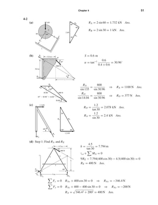
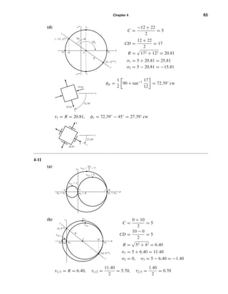
57. Chapter 4 57
10 ≤ x ≤ 15: V = 160 − 40x + 40(x − 8) + 352 = 192 lbf
M = 160x − 20x2
+ 20(x − 8) + 352(x − 10) = 192x − 2240
15 ≤ x ≤ 20: V = 160 − 40x + 40(x − 8) + 352 − 320 = −128 lbf
M = 160x − 20x2
− 20(x − 8) + 352(x − 10) − 320(x − 15)
= −128x + 2560
Plots of V and M are the same as in Prob. 4-3.
4-5 Solution depends upon the beam selected.
4-6
(a) Moment at center, xc = (l − 2a)/2
Mc =
w
2
l
2
(l − 2a) −
l
2
2
=
wl
2
l
4
− a
At reaction, |Mr | = wa2
/2
a = 2.25, l = 10 in, w = 100 lbf/in
Mc =
100(10)
2
10
4
− 2.25 = 125 lbf · in
Mr =
100(2.252
)
2
= 253.1 lbf · in Ans.
(b) Minimum occurs when Mc = |Mr |
wl
2
l
4
− a =
wa2
2
⇒ a2
+ al − 0.25l2
= 0
Taking the positive root
a =
1
2
−l + l2 + 4(0.25l2) =
l
2
√
2 − 1 = 0.2071l Ans.
for l = 10 in and w = 100 lbf, Mmin = (100/2)[(0.2071)(10)]2
= 214.5 lbf · in
4-7 For the ith wire from bottom, from summing forces vertically
(a)
Ti = (i + 1)W
From summing moments about point a,
Ma = W(l − xi ) − iW xi = 0
Giving,
xi =
l
i + 1
W iW
Ti
xi
a
shi20396_ch04.qxd 8/18/03 10:35 AM Page 57

58. 58 Solutions Manual • Instructor’s Solution Manual to Accompany Mechanical Engineering Design
So
W =
l
1 + 1
=
l
2
x =
l
2 + 1
=
l
3
y =
l
3 + 1
=
l
4
z =
l
4 + 1
=
l
5
(b) With straight rigid wires, the mobile is not stable. Any perturbation can lead to all wires
becoming collinear. Consider a wire of length l bent at its string support:
Ma = 0
Ma =
iWl
i + 1
cos α −
ilW
i + 1
cos β = 0
iWl
i + 1
(cos α − cos β) = 0
Moment vanishes when α = β for any wire. Consider a ccw rotation angle β, which
makes α → α + β and β → α − β
Ma =
iWl
i + 1
[cos(α + β) − cos(α − β)]
=
2iWl
i + 1
sin α sin β
.
=
2iWlβ
i + 1
sin α
There exists a correcting moment of opposite sense to arbitrary rotation β. An equation
for an upward bend can be found by changing the sign of W. The moment will no longer
be correcting. A curved, convex-upward bend of wire will produce stable equilibrium
too, but the equation would change somewhat.
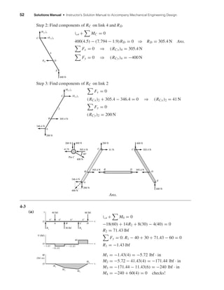
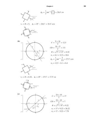
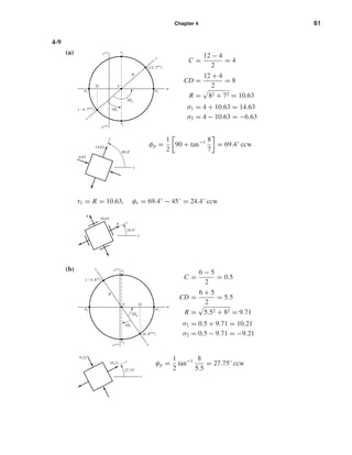
4-8
(a)
C =
12 + 6
2
= 9
CD =
12 − 6
2
= 3
R = 32 + 42 = 5
σ1 = 5 + 9 = 14
σ2 = 9 − 5 = 4
2␾s
(12, 4cw
)
C
R
D
␶2
␶1
␴1
␴␴2
2␾p
(6, 4ccw
)
y
x
␶cw
␶ccw
W
iW
il
i ϩ 1
Ti
␤␣
l
i ϩ 1
shi20396_ch04.qxd 8/18/03 10:35 AM Page 58

59. Chapter 4 59
φp =
1
2
tan−1 4
3
= 26.6◦
cw
τ1 = R = 5, φs = 45◦
− 26.6◦
= 18.4◦
ccw
(b)
C =
9 + 16
2
= 12.5
CD =
16 − 9
2
= 3.5
R = 52 + 3.52 = 6.10
σ1 = 6.1 + 12.5 = 18.6
φp =
1
2
tan−1 5
3.5
= 27.5◦
ccw
σ2 = 12.5 − 6.1 = 6.4
τ1 = R = 6.10, φs = 45◦
− 27.5◦
= 17.5◦
cw
(c)
C =
24 + 10
2
= 17
CD =
24 − 10
2
= 7
R = 72 + 62 = 9.22
σ1 = 17 + 9.22 = 26.22
σ2 = 17 − 9.22 = 7.78
2␾s
(24, 6cw
)
C
R
D
␶2
␶1
␴1␴2
2␾p
(10, 6ccw
)
y
x
␴
␶cw
␶ccw
x
12.5
12.5
6.10
17.5Њ
x
6.4
18.6
27.5Њ
2␾s
(16, 5ccw
)
C
R
D
␶2
␶1
␴1␴2
2␾p
(9, 5cw
)
y
x
␴
␶cw
␶ccw
3
5
3
3
3
18.4Њ
x
x
4
14
26.6Њ
shi20396_ch04.qxd 8/18/03 10:35 AM Page 59

60. 60 Solutions Manual • Instructor’s Solution Manual to Accompany Mechanical Engineering Design
φp =
1
2
90 + tan−1 7
6
= 69.7◦
ccw
τ1 = R = 9.22, φs = 69.7◦
− 45◦
= 24.7◦
ccw
(d)
C =
9 + 19
2
= 14
CD =
19 − 9
2
= 5
R = 52 + 82 = 9.434
σ1 = 14 + 9.43 = 23.43
σ2 = 14 − 9.43 = 4.57
φp =
1
2
90 + tan−1 5
8
= 61.0◦
cw
τ1 = R = 9.434, φs = 61◦
− 45◦
= 16◦
cw
x
14
14
9.434
16Њ
x
23.43
4.57
61Њ
2␾s
(9, 8cw
)
C
R
D
␶2
␶1
␴1␴2
2␾p
(19, 8ccw
)
y
x
␴
␶cw
␶ccw
x
17
17
9.22
24.7Њ
x
26.22
7.78
69.7Њ
shi20396_ch04.qxd 8/18/03 10:35 AM Page 60

61. Chapter 4 61
4-9
(a)
C =
12 − 4
2
= 4
CD =
12 + 4
2
= 8
R = 82 + 72 = 10.63
σ1 = 4 + 10.63 = 14.63
σ2 = 4 − 10.63 = −6.63
φp =
1
2
90 + tan−1 8
7
= 69.4◦
ccw
τ1 = R = 10.63, φs = 69.4◦
− 45◦
= 24.4◦
ccw
(b)
C =
6 − 5
2
= 0.5
CD =
6 + 5
2
= 5.5
R = 5.52 + 82 = 9.71
σ1 = 0.5 + 9.71 = 10.21
σ2 = 0.5 − 9.71 = −9.21
φp =
1
2
tan−1 8
5.5
= 27.75◦
ccw
x
10.21
9.21
27.75Њ
2␾s
(Ϫ5, 8cw
)
C
R
D
␶2
␶1
␴1
␴
␴2
2␾p
(6, 8ccw
)
y
x
␶cw
␶ccw
x
4
4
10.63
24.4Њ
x
14.63
6.63
69.4Њ
2␾s
(12, 7cw
)
C
R
D
␶2
␶1
␴1
␴␴2
2␾p
(Ϫ4, 7ccw
)
y
x
␶cw
␶ccw
shi20396_ch04.qxd 8/18/03 10:35 AM Page 61

62. 62 Solutions Manual • Instructor’s Solution Manual to Accompany Mechanical Engineering Design
τ1 = R = 9.71, φs = 45◦
− 27.75◦
= 17.25◦
cw
(c)
C =
−8 + 7
2
= −0.5
CD =
8 + 7
2
= 7.5
R = 7.52 + 62 = 9.60
σ1 = 9.60 − 0.5 = 9.10
σ2 = −0.5 − 9.6 = −10.1
φp =
1
2
90 + tan−1 7.5
6
= 70.67◦
cw
τ1 = R = 9.60, φs = 70.67◦
− 45◦
= 25.67◦
cw
(d)
C =
9 − 6
2
= 1.5
CD =
9 + 6
2
= 7.5
R = 7.52 + 32 = 8.078
σ1 = 1.5 + 8.078 = 9.58
σ2 = 1.5 − 8.078 = −6.58
2␾s
(9, 3cw
)
CR D
␶2
␶1
␴1␴2
2␾p
(Ϫ6, 3ccw
)
y
x
␴
␶cw
␶ccw
x
0.5
0.5
9.60
25.67Њ
x
10.1
9.1
70.67Њ
2␾s
(Ϫ8, 6cw
)
C
R
D
␶2
␶1
␴1␴2
2␾p
(7, 6ccw
)
x
y
␴
␶cw
␶ccw
x
0.5
0.5
9.71
17.25Њ
shi20396_ch04.qxd 8/18/03 10:35 AM Page 62

63. Chapter 4 63
φp =
1
2
tan−1 3
7.5
= 10.9◦
cw
τ1 = R = 8.078, φs = 45◦
− 10.9◦
= 34.1◦
ccw
4-10
(a)
C =
20 − 10
2
= 5
CD =
20 + 10
2
= 15
R = 152 + 82 = 17
σ1 = 5 + 17 = 22
σ2 = 5 − 17 = −12
φp =
1
2
tan−1 8
15
= 14.04◦
cw
τ1 = R = 17, φs = 45◦
− 14.04◦
= 30.96◦
ccw
5
17
5
30.96Њ
x
12
22
14.04Њ
x
2␾s (20, 8cw
)
C
R
D
␶2
␶1
␴1␴2
2␾p
(Ϫ10, 8ccw
)
y
x
␴
␶cw
␶ccw
x
1.5
8.08
1.5
34.1Њ
x
6.58
9.58
10.9Њ
shi20396_ch04.qxd 8/18/03 10:35 AM Page 63

64. 64 Solutions Manual • Instructor’s Solution Manual to Accompany Mechanical Engineering Design
(b)
C =
30 − 10
2
= 10
CD =
30 + 10
2
= 20
R = 202 + 102 = 22.36
σ1 = 10 + 22.36 = 32.36
σ2 = 10 − 22.36 = −12.36
φp =
1
2
tan−1 10
20
= 13.28◦
ccw
τ1 = R = 22.36, φs = 45◦
− 13.28◦
= 31.72◦
cw
(c)
C =
−10 + 18
2
= 4
CD =
10 + 18
2
= 14
R = 142 + 92 = 16.64
σ1 = 4 + 16.64 = 20.64
σ2 = 4 − 16.64 = −12.64
φp =
1
2
90 + tan−1 14
9
= 73.63◦
cw
τ1 = R = 16.64, φs = 73.63◦
− 45◦
= 28.63◦
cw
4
x
16.64
4
28.63Њ
12.64
20.64
73.63Њ
x
2␾s(Ϫ10, 9cw
)
C
R
D
␶2
␶1
␴1␴2
2␾p
(18, 9ccw
)
y
x
␴
␶cw
␶ccw
10
10
22.36
31.72Њ
x
12.36
32.36
x
13.28Њ
2␾s
(Ϫ10, 10cw
)
C
R
D
␶2
␶1
␴1
␴
␴2 2␾p
(30, 10ccw
)
y
x
␶cw
␶ccw
shi20396_ch04.qxd 8/18/03 10:35 AM Page 64

65. Chapter 4 65
(d)
C =
−12 + 22
2
= 5
CD =
12 + 22
2
= 17
R = 172 + 122 = 20.81
σ1 = 5 + 20.81 = 25.81
σ2 = 5 − 20.81 = −15.81
φp =
1
2
90 + tan−1 17
12
= 72.39◦
cw
τ1 = R = 20.81, φs = 72.39◦
− 45◦
= 27.39◦
cw
4-11
(a)
(b)
C =
0 + 10
2
= 5
CD =
10 − 0
2
= 5
R = 52 + 42 = 6.40
σ1 = 5 + 6.40 = 11.40
σ2 = 0, σ3 = 5 − 6.40 = −1.40
τ1/3 = R = 6.40, τ1/2 =
11.40
2
= 5.70, τ2/3 =
1.40
2
= 0.70
␴1␴2
␴
␴3
D
x
y
␶
C
R
(0, 4cw
)
(10, 4ccw
)
␶2/3
␶1/2
␶1/3
␴x ϭ ␴1
␴
␴3 ϭ ␴y
␶
␴2 ϭ 0
Ϫ4 10y x
␶2/3 ϭ 2
␶1/2 ϭ 5
␶1/3 ϭ ϭ 7
14
2
5
20.81
5
27.39Њ
x
15.81
25.81
72.39Њ
x
2␾s(Ϫ12, 12cw
)
C
R
D
␶2
␶1
␴1␴2
2␾p
(22, 12ccw
)
y
x
␴
␶cw
␶ccw
shi20396_ch04.qxd 8/18/03 10:35 AM Page 65

66. 66 Solutions Manual • Instructor’s Solution Manual to Accompany Mechanical Engineering Design
(c)
C =
−2 − 8
2
= −5
CD =
8 − 2
2
= 3
R = 32 + 42 = 5
σ1 = −5 + 5 = 0, σ2 = 0
σ3 = −5 − 5 = −10
τ1/3 =
10
2
= 5, τ1/2 = 0, τ2/3 = 5
(d)
C =
10 − 30
2
= −10
CD =
10 + 30
2
= 20
R = 202 + 102 = 22.36
σ1 = −10 + 22.36 = 12.36
σ2 = 0
σ3 = −10 − 22.36 = −32.36
τ1/3 = 22.36, τ1/2 =
12.36
2
= 6.18, τ2/3 =
32.36
2
= 16.18
4-12
(a)
C =
−80 − 30
2
= −55
CD =
80 − 30
2
= 25
R = 252 + 202 = 32.02
σ1 = 0
σ2 = −55 + 32.02 = −22.98 = −23.0
σ3 = −55 − 32.0 = −87.0
τ1/2 =
23
2
= 11.5, τ2/3 = 32.0, τ1/3 =
87
2
= 43.5
␴1
(Ϫ80, 20cw
)
(Ϫ30, 20ccw
)
C
D
R
␶2/3
␶1/2
␶1/3
␴2␴3
x
y
␶
␴
␴1
(Ϫ30, 10cw
)
(10, 10ccw
)
C D
R
␶2/3
␶1/2
␶␶1/3
␴2␴3
␴
y
x
␴1␴2
␴
␶
␴3
(Ϫ2, 4cw
)
Point is a circle
2 circles
C
D
y
x
(Ϫ8, 4ccw
)
shi20396_ch04.qxd 8/18/03 10:36 AM Page 66

67. Chapter 4 67
(b)
C =
30 − 60
2
= −15
CD =
60 + 30
2
= 45
R = 452 + 302 = 54.1
σ1 = −15 + 54.1 = 39.1
σ2 = 0
σ3 = −15 − 54.1 = −69.1
τ1/3 =
39.1 + 69.1
2
= 54.1, τ1/2 =
39.1
2
= 19.6, τ2/3 =
69.1
2
= 34.6
(c)
C =
40 + 0
2
= 20
CD =
40 − 0
2
= 20
R = 202 + 202 = 28.3
σ1 = 20 + 28.3 = 48.3
σ2 = 20 − 28.3 = −8.3
σ3 = σz = −30
τ1/3 =
48.3 + 30
2
= 39.1, τ1/2 = 28.3, τ2/3 =
30 − 8.3
2
= 10.9
(d)
C =
50
2
= 25
CD =
50
2
= 25
R = 252 + 302 = 39.1
σ1 = 25 + 39.1 = 64.1
σ2 = 25 − 39.1 = −14.1
σ3 = σz = −20
τ1/3 =
64.1 + 20
2
= 42.1, τ1/2 = 39.1, τ2/3 =
20 − 14.1
2
= 2.95
␴1
(50, 30cw
)
(0, 30ccw
)
C D
␶2/3
␶1/2
␶1/3
␴2␴3
x
y
␴
␶
␴1
(0, 20cw
)
(40, 20ccw
)
C
D
R
␶2/3
␶1/2
␶1/3
␴2␴3
y
x
␴
␶
␴1
␴
␶
(Ϫ60, 30ccw
)
(30, 30cw
)
C D
R
␶2/3
␶1/2
␶1/3
␴2␴3
x
y
shi20396_ch04.qxd 8/18/03 10:36 AM Page 67

68. 68 Solutions Manual • Instructor’s Solution Manual to Accompany Mechanical Engineering Design
4-13
σ =
F
A
=
2000
(π/4)(0.52)
= 10 190 psi = 10.19 kpsi Ans.
δ =
FL
AE
= σ
L
E
= 10 190
72
30(106)
= 0.024 46 in Ans.
1 =
δ
L
=
0.024 46
72
= 340(10−6
) = 340µ Ans.
From Table A-5, ν = 0.292
2 = −ν 1 = −0.292(340) = −99.3µ Ans.
d = 2d = −99.3(10−6
)(0.5) = −49.6(10−6
) in Ans.
4-14 From Table A-5, E = 71.7 GPa
δ = σ
L
E
= 135(106
)
3
71.7(109)
= 5.65(10−3
) m = 5.65 mm Ans.
4-15 From Table 4-2, biaxial case. From Table A-5, E = 207 GPa and ν = 0.292
σx =
E( x + ν y)
1 − ν2
=
207(109
)[0.0021 + 0.292(−0.000 67)]
1 − 0.2922
(10−6
) = 431 MPa Ans.
σy =
207(109
)[−0.000 67 + 0.292(0.0021)]
1 − 0.2922
(10−6
) = −12.9 MPa Ans.
4-16 The engineer has assumed the stress to be uniform. That is,
Ft = −F cos θ + τ A = 0 ⇒ τ =
F
A
cos θ
When failure occurs in shear
Ssu =
F
A
cos θ
The uniform stress assumption is common practice but is not exact. If interested in the
details, see p. 570 of 6th edition.
4-17 From Eq. (4-15)
σ3
− (−2 + 6 − 4)σ2
+ [−2(6) + (−2)(−4) + 6(−4) − 32
− 22
− (−5)2
]σ
− [−2(6)(−4) + 2(3)(2)(−5) − (−2)(2)2
− 6(−5)2
− (−4)(3)2
] = 0
σ3
− 66σ + 118 = 0
Roots are: 7.012, 1.89, −8.903 kpsi Ans.
␶
␴
t
␪
F
shi20396_ch04.qxd 8/18/03 10:36 AM Page 68

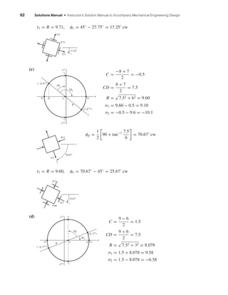
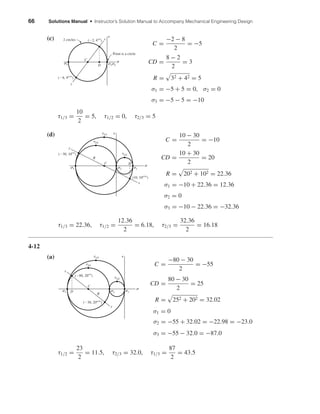
69. Chapter 4 69
τ1/2 =
7.012 − 1.89
2
= 2.56 kpsi
τ2/3 =
8.903 + 1.89
2
= 5.40 kpsi
τmax = τ1/3 =
8.903 + 7.012
2
= 7.96 kpsi Ans.
Note: For Probs. 4-17 to 4-19, one can also find the eigenvalues of the matrix
[σ] =
σx τxy τzx
τxy σy τyz
τzx τyz σz
for the principal stresses
4-18 From Eq. (4-15)
σ3
− (10 + 0 + 10)σ2
+ 10(0) + 10(10) + 0(10) − 202
− −10
√
2
2
− 02
σ
− 10(0)(10) + 2(20) −10
√
2 (0) − 10 −10
√
2
2
− 0(0)2
− 10(20)2
= 0
σ3
− 20σ2
− 500σ + 6000 = 0
Roots are: 30, 10, −20 MPa Ans.
τ1/2 =
30 − 10
2
= 10 MPa
τ2/3 =
10 + 20
2
= 15 MPa
τmax = τ1/3 =
30 + 20
2
= 25 MPa Ans.
4-19 From Eq. (4-15)
σ3
− (1 + 4 + 4)σ2
+ [1(4) + 1(4) + 4(4) − 22
− (−4)2
− (−2)2
]σ
−[1(4)(4) + 2(2)(−4)(−2) − 1(−4)2
− 4(−2)2
− 4(2)2
] = 0
σ3
− 9σ2
= 0
3010Ϫ20
␶2/3
␶1/2
␶1/3
␴ (MPa)
␶ (MPa)
7.0121.89
Ϫ8.903
␶2/3
␶1/2
␶1/3
␶ (kpsi)
␴ (kpsi)
shi20396_ch04.qxd 8/18/03 10:36 AM Page 69

70. 70 Solutions Manual • Instructor’s Solution Manual to Accompany Mechanical Engineering Design
Roots are: 9, 0, 0 kpsi
τ2/3 = 0, τ1/2 = τ1/3 = τmax =
9
2
= 4.5 kpsi Ans.
4-20
(a) R1 =
c
l
F Mmax = R1a =
ac
l
F
σ =
6M
bh2
=
6
bh2
ac
l
F ⇒ F =
σbh2
l
6ac
Ans.
(b)
Fm
F
=
(σm/σ)(bm/b) (hm/h)2
(lm/l)
(am/a) (cm/c)
=
1(s)(s)2
(s)
(s)(s)
= s2
Ans.
For equal stress, the model load varies by the square of the scale factor.
4-21
R1 =
wl
2
, Mmax|x=l/2 =
w
2
l
2
l −
l
2
=
wl2
8
σ =
6M
bh2
=
6
bh2
wl2
8
=
3Wl
4bh2
⇒ W =
4
3
σbh2
l
Ans.
Wm
W
=
(σm/σ)(bm/b) (hm/h)2
lm/l
=
1(s)(s)2
s
= s2
Ans.
wmlm
wl
= s2
⇒
wm
w
=
s2
s
= s Ans.
For equal stress, the model load w varies linearily with the scale factor.
4-22
(a) Can solve by iteration or derive equations for the general case.
Find maximum moment under wheel W3
WT = W at centroid of W’s
RA =
l − x3 − d3
l
WT
RA
W1
A B
W3 . . . . . .W2 WT
d3
Wn
RB
a23
a13
x3
l
␶2/3
␶(kpsi)
␴(kpsi)
␶1/2 ϭ ␶1/3
O 0 9
shi20396_ch04.qxd 8/18/03 10:36 AM Page 70

71. Chapter 4 71
Under wheel 3
M3 = RAx3 − W1a13 − W2a23 =
(l − x3 − d3)
l
WT x3 − W1a13 − W2a23
For maximum,
dM3
dx3
= 0 = (l − d3 − 2x3)
WT
l
⇒ x3 =
l − d3
2
substitute into M, ⇒ M3 =
(l − d3)2
4l
WT − W1a13 − W2a23
This means the midpoint of d3 intersects the midpoint of the beam
For wheel i xi =
l − di
2
, Mi =
(l − di )2
4l
WT −
i−1
j=1
Wjaji
Note for wheel 1: Wjaji = 0
WT = 104.4, W1 = W2 = W3 = W4 =
104.4
4
= 26.1 kip
Wheel 1: d1 =
476
2
= 238 in, M1 =
(1200 − 238)2
4(1200)
(104.4) = 20 128 kip · in
Wheel 2: d2 = 238 − 84 = 154 in
M2 =
(1200 − 154)2
4(1200)
(104.4) − 26.1(84) = 21 605 kip · in = Mmax
Check if all of the wheels are on the rail
(b) xmax = 600 − 77 = 523 in
(c) See above sketch.
(d) inner axles
4-23
(a)
Aa = Ab = 0.25(1.5) = 0.375 in2
A = 3(0.375) = 1.125 in2
1
2
1 " 1
4
"
3
8
"
1
4
"
1
4
"
D
C
1 1
Ga
Gb
c1 ϭ 0.833"
0.167"
0.083"
0.5"
0.75"
1.5"
y ϭ c2 ϭ 0.667"
B
aa
b
A
600" 600"
84" 77" 84"
315"
xmax
shi20396_ch04.qxd 8/18/03 10:36 AM Page 71

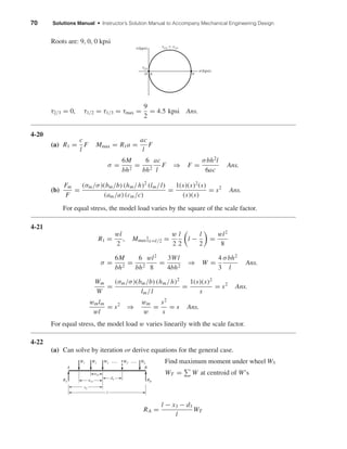
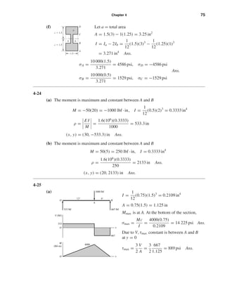
72. 72 Solutions Manual • Instructor’s Solution Manual to Accompany Mechanical Engineering Design
¯y =
2(0.375)(0.75) + 0.375(0.5)
1.125
= 0.667 in
Ia =
0.25(1.5)3
12
= 0.0703 in4
Ib =
1.5(0.25)3
12
= 0.001 95 in4
I1 = 2[0.0703 + 0.375(0.083)2
] + [0.001 95 + 0.375(0.167)2
] = 0.158 in4
Ans.
σA =
10 000(0.667)
0.158
= 42(10)3
psi Ans.
σB =
10 000(0.667 − 0.375)
0.158
= 18.5(10)3
psi Ans.
σC =
10 000(0.167 − 0.125)
0.158
= 2.7(10)3
psi Ans.
σD = −
10 000(0.833)
0.158
= −52.7(10)3
psi Ans.
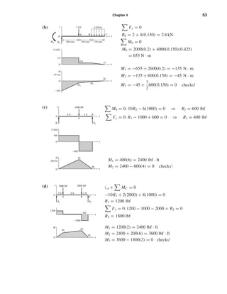
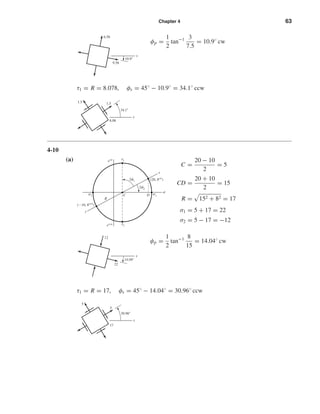
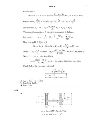
(b)
Here we treat the hole as a negative area.
Aa = 1.732 in2
Ab = 1.134
0.982
2
= 0.557 in2
A = 1.732 − 0.557 = 1.175 in2
¯y =
1.732(0.577) − 0.557(0.577)
1.175
= 0.577 in Ans.
Ia =
bh3
36
=
2(1.732)3
36
= 0.289 in4
Ib =
1.134(0.982)3
36
= 0.0298 in4
I1 = Ia − Ib = 0.289 − 0.0298 = 0.259 in4
Ans.
D
C
B
A
y
11
a b
A
Ga Gb0.327"
0.25"
c1 ϭ 1.155"
c2 ϭ 0.577"
2"
1.732"
0.577"
0.982"
0.577"
1.134"
shi20396_ch04.qxd 8/18/03 10:36 AM Page 72

73. Chapter 4 73
because the centroids are coincident.
σA =
10 000(0.577)
0.259
= 22.3(10)3
psi Ans.
σB =
10 000(0.327)
0.259
= 12.6(10)3
psi Ans.
σC = −
10 000(0.982 − 0.327)
0.259
= −25.3(10)3
psi Ans.
σD = −
10 000(1.155)
0.259
= −44.6(10)3
psi Ans.
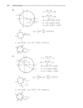
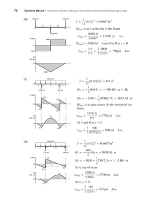
(c) Use two negative areas.
Aa = 1 in2
, Ab = 9 in2
, Ac = 16 in2
, A = 16 − 9 − 1 = 6 in2
;
¯ya = 0.25 in, ¯yb = 2.0 in, ¯yc = 2 in
¯y =
16(2) − 9(2) − 1(0.25)
6
= 2.292 in Ans.
c1 = 4 − 2.292 = 1.708 in
Ia =
2(0.5)3
12
= 0.020 83 in4
Ib =
3(3)3
12
= 6.75 in4
Ic =
4(4)3
12
= 21.333 in4
I1 = [21.333 + 16(0.292)2
] − [6.75 + 9(0.292)2
]
− [0.020 83 + 1(2.292 − 0.25)2
]
= 10.99 in4
Ans.
σA =
10 000(2.292)
10.99
= 2086 psi Ans.
σB =
10 000(2.292 − 0.5)
10.99
= 1631 psi Ans.
σC = −
10 000(1.708 − 0.5)
10.99
= −1099 psi Ans.
σD = −
10 000(1.708)
10.99
= −1554 psi Ans.
D
C
c
a
B
b
A
Ga
Gb Gc
c1 ϭ 1.708"
c2 ϭ 2.292"
2"
1.5"
0.25"
11
shi20396_ch04.qxd 8/18/03 10:36 AM Page 73

74. 74 Solutions Manual • Instructor’s Solution Manual to Accompany Mechanical Engineering Design
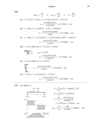
(d) Use a as a negative area.
Aa = 6.928 in2
, Ab = 16 in2
, A = 9.072 in2
;
¯ya = 1.155 in, ¯yb = 2 in
¯y =
2(16) − 1.155(6.928)
9.072
= 2.645 in Ans.
c1 = 4 − 2.645 = 1.355 in
Ia =
bh3
36
=
4(3.464)3
36
= 4.618 in4
Ib =
4(4)3
12
= 21.33 in4
I1 = [21.33 + 16(0.645)2
] − [4.618 + 6.928(1.490)2
]
= 7.99 in4
Ans.
σA =
10 000(2.645)
7.99
= 3310 psi Ans.
σB = −
10 000(3.464 − 2.645)
7.99
= −1025 psi Ans.
σC = −
10 000(1.355)
7.99
= −1696 psi Ans.
(e) Aa = 6(1.25) = 7.5 in2
Ab = 3(1.5) = 4.5 in2
A = Ac + Ab = 12 in2
¯y =
3.625(7.5) + 1.5(4.5)
12
= 2.828 in Ans.
I =
1
12
(6)(1.25)3
+ 7.5(3.625 − 2.828)2
+
1
12
(1.5)(3)3
+ 4.5(2.828 − 1.5)2
= 17.05 in4
Ans.
σA =
10 000(2.828)
17.05
= 1659 psi Ans.
σB = −
10 000(3 − 2.828)
17.05
= −101 psi Ans.
σC = −
10 000(1.422)
17.05
= −834 psi Ans.
a
b
A
B
C
c1 ϭ 1.422"
c2 ϭ 2.828"
3.464"
11
Ga
B
b
a
C
A
c1 ϭ 1.355"
c2 ϭ 2.645"
1.490"
1.155"
shi20396_ch04.qxd 8/18/03 10:36 AM Page 74

75. Chapter 4 75
(f) Let a = total area
A = 1.5(3) − 1(1.25) = 3.25 in2
I = Ia − 2Ib =
1
12
(1.5)(3)3
−
1
12
(1.25)(1)3
= 3.271 in4
Ans.
σA =
10 000(1.5)
3.271
= 4586 psi, σD = −4586 psi
Ans.
σB =
10 000(0.5)
3.271
= 1529 psi, σC = −1529 psi
4-24
(a) The moment is maximum and constant between A and B
M = −50(20) = −1000 lbf · in, I =
1
12
(0.5)(2)3
= 0.3333 in4
ρ =
E I
M
=
1.6(106
)(0.3333)
1000
= 533.3 in
(x, y) = (30, −533.3) in Ans.
(b) The moment is maximum and constant between A and B
M = 50(5) = 250 lbf · in, I = 0.3333 in4
ρ =
1.6(106
)(0.3333)
250
= 2133 in Ans.
(x, y) = (20, 2133) in Ans.
4-25
(a)
I =
1
12
(0.75)(1.5)3
= 0.2109 in4
A = 0.75(1.5) = 1.125 in
Mmax is at A. At the bottom of the section,
σmax =
Mc
I
=
4000(0.75)
0.2109
= 14 225 psi Ans.
Due to V, τmax constant is between A and B
at y = 0
τmax =
3
2
V
A
=
3
2
667
1.125
= 889 psi Ans.
1000 lbf
4000
333 lbf 667 lbf
O B
x
A
O
333
667
O
12" 6"
V (lbf)
M
(lbf•in)
x
C
B
A
b
a
b
D
c ϭ 1.5
c ϭ 1.5
1.5
shi20396_ch04.qxd 8/18/03 10:36 AM Page 75

76. 76 Solutions Manual • Instructor’s Solution Manual to Accompany Mechanical Engineering Design
(b)
I =
1
12
(1)(2)3
= 0.6667 in4
Mmax is at A at the top of the beam
σmax =
8000(1)
0.6667
= 12 000 psi Ans.
|Vmax| = 1000 lbf from O to B at y = 0
τmax =
3
2
V
A
=
3
2
1000
(2)(1)
= 750 psi Ans.
(c)
I =
1
12
(0.75)(2)3
= 0.5 in4
M1 = −
1
2
600(5) = −1500 lbf · in = M3
M2 = −1500 +
1
2
(900)(7.5) = 1875 lbf · in
Mmax is at span center. At the bottom of the
beam,
σmax =
1875(1)
0.5
= 3750 psi Ans.
At A and B at y = 0
τmax =
3
2
900
(0.75)(2)
= 900 psi Ans.
(d)
I =
1
12
(1)(2)3
= 0.6667 in4
M1 = −
600
2
(6) = −1800 lbf · in
M2 = −1800 +
1
2
750(7.5) = 1013 lbf · in
At A, top of beam
σmax =
1800(1)
0.6667
= 2700 psi Ans.
At A, y = 0
τmax =
3
2
750
(2)(1)
= 563 psi Ans.
100 lbf/in
1350 lbf 450 lbf
O BA
O
O
V (lbf)
M
(lbf•in)
6" 12"
7.5"
750
M1
M2
Ϫ450
Ϫ600
x
x
x
120 lbf/in
1500 lbf 1500 lbf
O
CBA
O
O
V (lbf)
M
(lbf•in)
5" 15" 5"
900
M1
M2
x
M3
Ϫ900
Ϫ600
600
x
x
1000 lbf 1000 lbf
1000
Ϫ1000
Ϫ8000
2000 lbf
O B
A
O
O
8" 8"
V (lbf)
M
(lbf•in)
x
x
x
shi20396_ch04.qxd 8/18/03 10:36 AM Page 76

77. Chapter 4 77
4-26
Mmax =
wl2
8
⇒ σmax =
wl2
c
8I
⇒ w =
8σ I
cl2
(a) l = 12(12) = 144 in, I = (1/12)(1.5)(9.5)3
= 107.2 in4
w =
8(1200)(107.2)
4.75(1442)
= 10.4 lbf/in Ans.
(b) l = 48 in, I = (π/64)(24
− 1.254
) = 0.6656 in4
w =
8(12)(103
)(0.6656)
1(48)2
= 27.7 lbf/in Ans.
(c) l = 48 in, I
.
= (1/12)(2)(33
) − (1/12)(1.625)(2.6253
) = 2.051 in4
w =
8(12)(103
)(2.051)
1.5(48)2
= 57.0 lbf/in Ans.
(d) l = 72 in; Table A-6, I = 2(1.24) = 2.48 in4
cmax = 2.158"
w =
8(12)(103
)(2.48)
2.158(72)2
= 21.3 lbf/in Ans.
(e) l = 72 in; Table A-7, I = 3.85 in4
w =
8(12)(103
)(3.85)
2(722)
= 35.6 lbf/in Ans.
(f) l = 72 in, I = (1/12)(1)(43
) = 5.333 in4
w =
8(12)(103
)(5.333)
(2)(72)2
= 49.4 lbf/in Ans.
4-27 (a) Model (c)
I =
π
64
(0.54
) = 3.068(10−3
) in4
A =
π
4
(0.52
) = 0.1963 in2
σ =
Mc
I
=
218.75(0.25)
3.068(10−3)
= 17 825 psi = 17.8 kpsi Ans.
τmax =
4
3
V
A
=
4
3
500
0.1963
= 3400 psi Ans.
1.25 in
500 lbf 500 lbf
500 lbf500 lbf
0.4375
500
Ϫ500
O
V (lbf)
O
M
(lbf¥in)
Mmax ϭ 500(0.4375)
ϭ 218.75 lbf¥in
2
0.842"
2.158"
shi20396_ch04.qxd 8/18/03 10:36 AM Page 77

78. 78 Solutions Manual • Instructor’s Solution Manual to Accompany Mechanical Engineering Design
(b) Model (d)
Mmax = 500(0.25) +
1
2
(500)(0.375)
= 218.75 lbf · in
Vmax = 500 lbf
Same M and V
∴ σ = 17.8 kpsi Ans.
τmax = 3400 psi Ans.
4-28 If support RB is between F1 and F2 at position x = l, maximum moments occur at x = 3 and l.
MB = RAl − 2000(l − 3) + 1100(7.75 − l) = 0
RA = 3100 − 14 525/l
Mx=3 = 3RA = 9300 − 43 575/l
MB = RAl − 2000(l − 3) = 1100l − 8525
To minimize the moments, equate Mx=3 to −MB giving
9300 − 43 575/l = −1100l + 8525
Multiply by l and simplify to
l2
+ 0.7046l − 39.61 = 0
The positive solution for l is 5.95 in and the magnitude of the moment is
M = 9300 − 43 575/5.95 = 1976 lbf · in
Placing the bearing to the right of F2, the bending moment would be minimized by placing
it as close as possible to F2. If the bearing is near point B as in the original figure, then we
need to equate the reaction forces. From statics, RB = 14 525/l, and RA = 3100 − RB.
For RA = RB, then RA = RB = 1550 lbf, and l = 14 575/1550 = 9.37 in.
4-29
q = −F x −1
+ p1 x − l 0
−
p1 + p2
a
x − l 1
+ terms for x > l + a
V = −F + p1 x − l 1
−
p1 + p2
2a
x − l 2
+ terms for x > l + a
M = −Fx +
p1
2
x − l 2
−
p1 + p2
6a
x − l 3
+ terms for x > l + a
l p2
p1
a
b
F
1.25"
500 lbf 500 lbf
0.25"
1333 lbf/in
500
Ϫ500
O
V (lbf)
O
M Mmax
shi20396_ch04.qxd 8/18/03 10:36 AM Page 78

79. Chapter 4 79
At x = (l + a)+
, V = M = 0, terms for x > l + a = 0
−F + p1a −
p1 + p2
2a
a2
= 0 ⇒ p1 − p2 =
2F
a
(1)
−F(l + a) +
p1a2
2
−
p1 + p2
6a
a3
= 0 ⇒ 2p1 − p2 =
6F(l + a)
a2
(2)
From (1) and (2) p1 =
2F
a2
(3l + 2a), p2 =
2F
a2
(3l + a) (3)
From similar triangles
b
p2
=
a
p1 + p2
⇒ b =
ap2
p1 + p2
(4)
Mmax occurs where V = 0
xmax = l + a − 2b
Mmax = −F(l + a − 2b) +
p1
2
(a − 2b)2
−
p1 + p2
6a
(a − 2b)3
= −Fl − F(a − 2b) +
p1
2
(a − 2b)2
−
p1 + p2
6a
(a − 2b)3
Normally Mmax = −Fl
The fractional increase in the magnitude is
=
F(a − 2b) − ( p1/2)(a − 2b)2
− [( p1 + p2)/6a](a − 2b)3
Fl
(5)
For example, consider F = 1500 lbf, a = 1.2 in, l = 1.5 in
(3) p1 =
2(1500)
1.22
[3(1.5) + 2(1.2)] = 14 375 lbf/in
p2 =
2(1500)
1.22
[3(1.5) + 1.2] = 11 875 lbf/in
(4) b = 1.2(11 875)/(14 375 + 11 875) = 0.5429 in
Substituting into (5) yields
= 0.036 89 or 3.7% higher than −Fl
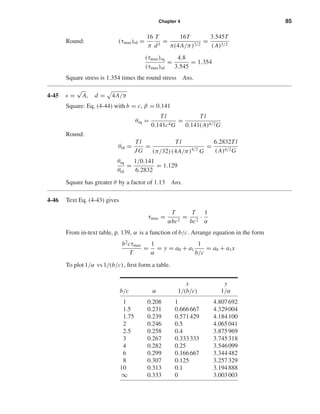
4-30 Computer program; no solution given here.
a Ϫ 2bl
F
p2
p2
p1
p2
b b
shi20396_ch04.qxd 8/18/03 10:36 AM Page 79

80. 80 Solutions Manual • Instructor’s Solution Manual to Accompany Mechanical Engineering Design
4-31
R1 =
c
l
F
M =
c
l
Fx 0 ≤ x ≤ a
σ =
6M
bh2
=
6(c/l)Fx
bh2
⇒ h =
6cFx
blσmax
0 ≤ x ≤ a Ans.
4-32
R1 =
b
l
F
M =
b
l
Fx
σmax =
32M
πd3
=
32
πd3
b
l
Fx
d =
32
π
bFx
lσmax
1/3
0 ≤ x ≤ a Ans.
4-33
Square: Am = (b − t)2
Tsq = 2Amtτall = 2(b − t)2
tτall
Round: Am = π(b − t)2
/4
Trd = 2π(b − t)2
tτall/4
Ratio of torques
Tsq
Trd
=
2(b − t)2
tτall
π(b − t)2tτall/2
=
4
π
= 1.27
Twist per unit length
square:
θsq =
2Gθ1t
tτall
L
A m
= C
L
A m
= C
4(b − t)
(b − t)2
Round:
θrd = C
L
A m
= C
π(b − t)
π(b − t)2/4
= C
4(b − t)
(b − t)2
Ratio equals 1, twists are the same.
t
b
t
b
R1
F
a b
l
R2
x
y
R1 R2
F
a c
l
shi20396_ch04.qxd 8/18/03 10:36 AM Page 80

81. Chapter 4 81
Note the weight ratio is
Wsq
Wrd
=
ρl(b − t)2
ρlπ(b − t)(t)
=
b − t
πt
thin-walled assumes b ≥ 20t
=
19
π
= 6.04 with b = 20
= 2.86 with b = 10t
4-34 l = 40 in, τall = 11 500 psi, G = 11.5(106
) psi, t = 0.050 in
rm = ri + t/2 = ri + 0.025 for ri > 0
= 0 for ri = 0
Am = (1 − 0.05)2
− 4 r2
m −
π
4
r2
m = 0.952
− (4 − π)r2
m
Lm = 4(1 − 0.05 − 2rm + 2πrm/4) = 4[0.95 − (2 − π/2)rm]
Eq. (4-45): T = 2Amtτ = 2(0.05)(11 500)Am = 1150Am
Eq. (4-46):
θ(deg) = θ1 l
180
π
=
T Lml
4G A2
mt
180
π
=
T Lm(40)
4(11.5)(106)A2
m(0.05)
180
π
= 9.9645(10−4
)
T Lm
A2
m
Equations can then be put into a spreadsheet resulting in:
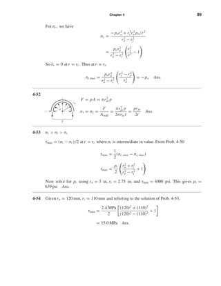
ri rm Am Lm ri T(lbf · in) ri θ(deg)
0 0 0.9025 3.8 0 1037.9 0 4.825
0.10 0.125 0.889087 3.585398 0.10 1022.5 0.10 4.621
0.20 0.225 0.859043 3.413717 0.20 987.9 0.20 4.553
0.30 0.325 0.811831 3.242035 0.30 933.6 0.30 4.576
0.40 0.425 0.747450 3.070354 0.40 859.6 0.40 4.707
0.45 0.475 0.708822 2.984513 0.45 815.1 0.45 4.825
ri (in)
T(lbf•in)
0
400
200
600
800
1000
1200
0 0.30.20.1 0.4 0.5
shi20396_ch04.qxd 8/18/03 10:36 AM Page 81

82. 82 Solutions Manual • Instructor’s Solution Manual to Accompany Mechanical Engineering Design
Torque carrying capacity reduces with ri . However, this is based on an assumption of uni-
form stresses which is not the case for smallri . Also note that weight also goes down with
an increase in ri .
4-35 From Eq. (4-47) where θ1 is the same for each leg.
T1 =
1
3
Gθ1L1c3
1, T2 =
1
3
Gθ1L2c3
2
T = T1 + T2 =
1
3
Gθ1 L1c3
1 + L2c3
2 =
1
3
Gθ1 Li c3
i Ans.
τ1 = Gθ1c1, τ2 = Gθ1c2
τmax = Gθ1cmax Ans.
4-36
(a) τmax = Gθ1cmax
Gθ1 =
τmax
cmax
=
11 500
3/32
= 1.227(105
) psi · rad
T1/16 =
1
3
Gθ1(Lc3
)1/16 =
1
3
(1.227)(105
)(0.5)(1/16)3
= 4.99 lbf · in Ans.
T3/32 =
1
3
(1.227)(105
)(0.5)(3/32)3
= 16.85 lbf · in Ans.
τ1/16 = 1.227(105
)1/16 = 7669 psi, τ3/32 = 1.227(105
)3/32 = 11 500 psi Ans.
(b) θ1 =
1.227(105
)
11.5(106)
= 1.0667(10−2
) rad/in = 0.611◦/in Ans.
4-37 Separate strips: For each 1/16 in thick strip,
T =
Lc2
τ
3
=
(1)(1/16)2
(11 500)
3
= 14.97 lbf · in
∴ Tmax = 2(14.97) = 29.95 lbf · in Ans.
ri (in)
␪(deg)
4.50
4.55
4.65
4.60
4.70
4.75
4.80
4.85
0 0.30.20.1 0.4 0.5
shi20396_ch04.qxd 8/18/03 10:36 AM Page 82

83. Chapter 4 83
For each strip,
θ =
3Tl
Lc3G
=
3(14.97)(12)
(1)(1/16)3(11.5)(106)
= 0.192 rad Ans.
kt = T/θ = 29.95/0.192 = 156.0 lbf · in Ans.
Solid strip: From Example 4-12,
Tmax = 59.90 lbf · in Ans.
θ = 0.0960 rad Ans.
kt = 624 lbf · in Ans.
4-38 τall = 8000 psi, 50 hp
(a) n = 2000 rpm
Eq. (4-40) T =
63 025H
n
=
63 025(50)
2000
= 1575.6 lbf · in
τmax =
16T
πd3
⇒ d =
16T
πτmax
1/3
=
16(1575.6)
π(8000)
1/3
= 1.00 in Ans.
(b) n = 200 rpm ∴ T = 15756 lbf · in
d =
16(15 756)
π(8000)
1/3
= 2.157 in Ans.
4-39 τall = 110 MPa, θ = 30◦
, d = 15 mm, l = ?
τ =
16T
πd3
⇒ T =
π
16
τd3
θ =
Tl
JG
180
π
l =
π
180
JGθ
T
=
π
180
π
32
d4
Gθ
(π/16) τd3
=
π
360
dGθ
τ
=
π
360
(0.015)(79.3)(109
)(30)
110(106)
= 2.83 m Ans.
4-40 d = 70 mm, replaced by 70 mm hollow with t = 6 mm
(a) Tsolid =
π
16
τ(703
) Thollow =
π
32
τ
(704
− 584
)
35
% T =
(π/16)(703) − (π/32) [(704 − 584)/35]
(π/16)(703)
(100) = 47.1% Ans.
shi20396_ch04.qxd 8/18/03 10:36 AM Page 83

84. 84 Solutions Manual • Instructor’s Solution Manual to Accompany Mechanical Engineering Design
(b) Wsolid = kd2
= k(702
), Whollow = k(702
− 582
)
% W =
k(702
) − k(702
− 582
)
k(702)
(100) = 68.7% Ans.
4-41 T = 5400 N · m, τall = 150 MPa
(a) τ =
Tc
J
⇒ 150(106
) =
5400(d/2)
(π/32)[d4 − (0.75d)4]
=
4.023(104
)
d3
d =
4.023(104
)
150(106)
1/3
= 6.45(10−2
)m = 64.5 mm
From Table A-17, the next preferred size is d = 80 mm; ID = 60 mm Ans.
(b) J =
π
32
(0.084
− 0.064
) = 2.749(10−6
) mm4
τi =
5400(0.030)
2.749(10−6)
= 58.9(106
) Pa = 58.9 MPa Ans.
4-42
(a) T =
63 025H
n
=
63 025(1)
5
= 12 605 lbf · in
τ =
16T
πd3
C
⇒ dC =
16T
πτ
1/3
=
16(12 605)
π(14 000)
1/3
= 1.66 in Ans.
From Table A-17, select 1 3/4 in
τstart =
16(2)(12 605)
π(1.753)
= 23.96(103
) psi = 23.96 kpsi
(b) design activity
4-43 ω = 2πn/60 = 2π(8)/60 = 0.8378 rad/s
T =
H
ω
=
1000
0.8378
= 1194 N · m
dC =
16T
πτ
1/3
=
16(1194)
π(75)(106)
1/3
= 4.328(10−2
) m = 43.3 mm
From Table A-17, select 45 mm Ans.
4-44 s =
√
A, d = 4A/π
Square: Eq. (4-43) with b = c
τmax =
4.8T
c3
(τmax)sq =
4.8T
(A)3/2
shi20396_ch04.qxd 8/18/03 10:36 AM Page 84

85. Chapter 4 85
Round: (τmax)rd =
16
π
T
d3
=
16T
π(4A/π)3/2
=
3.545T
(A)3/2
(τmax)sq
(τmax)rd
=
4.8
3.545
= 1.354
Square stress is 1.354 times the round stress Ans.
4-45 s =
√
A, d = 4A/π
Square: Eq. (4-44) with b = c, β = 0.141
θsq =
Tl
0.141c4G
=
Tl
0.141(A)4/2G
Round:
θrd =
Tl
JG
=
Tl
(π/32) (4A/π)4/2
G
=
6.2832Tl
(A)4/2G
θsq
θrd
=
1/0.141
6.2832
= 1.129
Square has greater θ by a factor of 1.13 Ans.
4-46 Text Eq. (4-43) gives
τmax =
T
αbc2
=
T
bc2
·
1
α
From in-text table, p. 139, α is a function of b/c. Arrange equation in the form
b2
cτmax
T
=
1
α
= y = a0 + a1
1
b/c
= a0 + a1x
To plot 1/α vs 1/(b/c), first form a table.
x y
b/c α 1/(b/c) 1/α
1 0.208 1 4.807692
1.5 0.231 0.666667 4.329004
1.75 0.239 0.571429 4.184100
2 0.246 0.5 4.065041
2.5 0.258 0.4 3.875969
3 0.267 0.333333 3.745318
4 0.282 0.25 3.546099
6 0.299 0.166667 3.344482
8 0.307 0.125 3.257329
10 0.313 0.1 3.194888
∞ 0.333 0 3.003003
shi20396_ch04.qxd 8/18/03 10:36 AM Page 85

86. 86 Solutions Manual • Instructor’s Solution Manual to Accompany Mechanical Engineering Design
Plot is a gentle convex-upward curve. Roark uses a polynomial, which in our notation is
τmax =
3T
8(b/2)(c/2)2
1 + 0.6095
1
b/c
+ · · ·
τmax
.
=
T
bc2
3 + 1.8285
1
b/c
Linear regression on table data
y = 3.06 + 1.87x
1
α
= 3.06 + 1.87
1
b/c
τmax =
T
bc2
3.06 + 1.87
1
b/c
Eq. (4-43) τmax =
T
bc2
3 +
1.8
b/c
4-47
Ft =
1000
2.5
= 400 lbf
Fn = 400 tan 20 = 145.6 lbf
Torque at C TC = 400(5) = 2000 lbf · in
P =
2000
3
= 666.7 lbf
10"
C
1000 lbf•in
2.5R
Ft
Fn ␾
Gear F
y
z
A
RAy
RAz
3"
Shaft ABCD
B
666.7 lbf
D x
5"400 lbf
145.6 lbf
C
RDy
RDz
2000 lbf•in
2000 lbf•in
1͞(b͞c)
1͞␣
3
3.5
4
4.5
5
0 0.60.40.2 0.8 1
y ϭ 1.867x ϩ 3.061
shi20396_ch04.qxd 8/18/03 10:36 AM Page 86

87. Chapter 4 87
(MA)z = 0 ⇒ 18RDy − 145.6(13) − 666.7(3) = 0 ⇒ RDy = 216.3 lbf
(MA)y = 0 ⇒ −18RDz + 400(13) = 0 ⇒ RDz = 288.9 lbf
Fy = 0 ⇒ RAy + 216.3 − 666.7 − 145.6 = 0 ⇒ RAy = 596.0 lbf
Fz = 0 ⇒ RAz + 288.9 − 400 = 0 ⇒ RAz = 111.1 lbf
MB = 3 5962 + 111.12 = 1819 lbf · in
MC = 5 216.32 + 288.92 = 1805 lbf · in
∴ Maximum stresses occur at B. Ans.
σB =
32MB
πd3
=
32(1819)
π(1.253)
= 9486 psi
τB =
16TB
πd3
=
16(2000)
π(1.253)
= 5215 psi
σmax =
σB
2
+
σB
2
2
+ τ2
B =
9486
2
+
9486
2
2
+ 52152 = 11 792 psi Ans.
τmax =
σB
2
2
+ τ2
B = 7049 psi Ans.
4-48
(a) At θ = 90◦
, σr = τrθ = 0, σθ = −σ Ans.
θ = 0◦
, σr = τrθ = 0, σθ = 3σ Ans.
(b)
r σθ /σ
5 3.000
6 2.071
7 1.646
8 1.424
9 1.297
10 1.219
11 1.167
12 1.132
13 1.107
14 1.088
15 1.074
16 1.063
17 1.054
18 1.048
19 1.042
20 1.037
r (mm)
␴␪͞␴
0
1
0.5
1.5
2
2.5
3
0 105 15 20
shi20396_ch04.qxd 8/18/03 10:36 AM Page 87

88. 88 Solutions Manual • Instructor’s Solution Manual to Accompany Mechanical Engineering Design
4-49
D/d =
1.5
1
= 1.5
r/d =
1/8
1
= 0.125
Fig. A-15-8: Kts
.
= 1.39
Fig. A-15-9: Kt
.
= 1.60
σA = Kt
Mc
I
=
32Kt M
πd3
=
32(1.6)(200)(14)
π(13)
= 45 630 psi
τA = Kts
Tc
J
=
16KtsT
πd3
=
16(1.39)(200)(15)
π(13)
= 21 240 psi
σmax =
σA
2
+
σA
2
2
+ τ2
A =
45.63
2
+
45.63
2
2
+ 21.242
= 54.0 kpsi Ans.
τmax =
45.63
2
2
+ 21.242 = 31.2 kpsi Ans.
4-50 As shown in Fig. 4-34, the maximum stresses occur at the inside fiber wherer = ri . There-
fore, from Eq. (4-51)
σt,max =
r2
i pi
r2
o − r2
i
1 +
r2
o
r2
i
= pi
r2
o + r2
i
r2
o − r2
i
Ans.
σr,max =
r2
i pi
r2
o − r2
i
1 −
r2
o
r2
i
= −pi Ans.
4-51 If pi = 0, Eq. (4-50) becomes
σt =
−por2
o − r2
i r2
o po/r2
r2
o − r2
i
= −
por2
o
r2
o − r2
i
1 +
r2
i
r2
The maximum tangential stress occurs at r = ri . So
σt,max = −
2por2
o
r2
o − r2
i
Ans.
shi20396_ch04.qxd 8/18/03 10:36 AM Page 88

89. Chapter 4 89
For σr , we have
σr =
−por2
o + r2
i r2
o po/r2
r2
o − r2
i
=
por2
o
r2
o − r2
i
r2
i
r2
− 1
So σr = 0 at r = ri . Thus at r = ro
σr,max =
por2
o
r2
o − r2
i
r2
i − r2
o
r2
o
= −po Ans.
4-52
F = pA = πr2
av p
σ1 = σ2 =
F
Awall
=
πr2
av p
2πravt
=
prav
2t
Ans.
4-53 σt > σl > σr
τmax = (σt − σr )/2 at r = ri where σl is intermediate in value. From Prob. 4-50
τmax =
1
2
(σt, max − σr, max)
τmax =
pi
2
r2
o + r2
i
r2
o − r2
i
+ 1
Now solve for pi using ro = 3 in, ri = 2.75 in, and τmax = 4000 psi. This gives pi =
639 psi Ans.
4-54 Given ro = 120 mm, ri = 110 mm and referring to the solution of Prob. 4-53,
τmax =
2.4 MPa
2
(120)2
+ (110)2
(120)2 − (110)2
+ 1
= 15.0 MPa Ans.
rav
p
t
F
shi20396_ch04.qxd 8/18/03 10:36 AM Page 89

90. 90 Solutions Manual • Instructor’s Solution Manual to Accompany Mechanical Engineering Design
4-55 From Table A-20, Sy = 57 kpsi; also, ro = 0.875 in and ri = 0.625 in
From Prob. 4-51
σt,max = −
2por2
o
r2
o − r2
i
Rearranging
po =
r2
o − r2
i (0.8Sy)
2r2
o
Solving, gives po = 11 200 psi Ans.
4-56 From Table A-20, Sy = 57 kpsi; also ro = 1.1875 in, ri = 0.875 in.
From Prob. 4-50
σt,max = pi
r2
o + r2
i
r2
o − r2
i
therefore pi = 0.8Sy
r2
o − r2
i
r2
o + r2
i
solving gives pi = 13 510 psi Ans.
4-57 Since σt and σr are both positive and σt > σr
τmax = (σt)max/2
where σt is max at ri
Eq. (4-56) for r = ri = 0.375 in
(σt)max =
0.282
386
2π(7200)
60
2
3 + 0.292
8
× 0.3752
+ 52
+
(0.3752
)(52
)
0.3752
−
1 + 3(0.292)
3 + 0.292
(0.3752
) = 8556 psi
τmax =
8556
2
= 4278 psi Ans.
Radial stress: σr = k r2
i + r2
o −
r2
i r2
o
r2
− r2
Maxima:
dσr
dr
= k 2
r2
i r2
o
r3
− 2r = 0 ⇒ r =
√
riro = 0.375(5) = 1.3693 in
(σr )max =
0.282
386
2π(7200)
60
2
3 + 0.292
8
0.3752
+ 52
−
0.3752
(52
)
1.36932
− 1.36932
= 3656 psi Ans.
shi20396_ch04.qxd 8/18/03 10:36 AM Page 90

91. Chapter 4 91
4-58 ω = 2π(2069)/60 = 216.7 rad/s,
ρ = 3320 kg/m3
, ν = 0.24, ri = 0.0125 m, ro = 0.15 m;
use Eq. (4-56)
σt = 3320(216.7)2 3 + 0.24
8
(0.0125)2
+ (0.15)2
+ (0.15)2
−
1 + 3(0.24)
3 + 0.24
(0.0125)2
(10)−6
= 2.85 MPa Ans.
4-59
ρ =
(6/16)
386(1/16)(π/4)(62 − 12)
= 5.655(10−4
) lbf · s2
/in
4
τmax is at bore and equals
σt
2
Eq. (4-56)
(σt)max = 5.655(10−4
)
2π(10 000)
60
2
3 + 0.20
8
0.52
+ 32
+ 32
−
1 + 3(0.20)
3 + 0.20
(0.5)2
= 4496 psi
τmax =
4496
2
= 2248 psi Ans.
4-60 ω = 2π(3000)/60 = 314.2 rad/s
m =
0.282(1.25)(12)(0.125)
386
= 1.370(10−3
) lbf · s2
/in
F = mω2
r = 1.370(10−3
)(314.22
)(6)
= 811.5 lbf
Anom = (1.25 − 0.5)(1/8) = 0.093 75 in2
σnom =
811.5
0.093 75
= 8656 psi Ans.
Note: Stress concentration Fig. A-15-1 gives Kt
.
= 2.25 which increases σmax and fatigue.
6"
F
␻
F
shi20396_ch04.qxd 8/18/03 10:36 AM Page 91

92. 92 Solutions Manual • Instructor’s Solution Manual to Accompany Mechanical Engineering Design
4-61 to 4-66
ν = 0.292, E = 30 Mpsi (207 GPa), ri = 0
R = 0.75 in (20 mm), ro = 1.5 in (40 mm)
Eq. (4-60)
ppsi =
30(106
)δ
0.75 in
(1.52
− 0.752
)(0.752
− 0)
2(0.752)(1.52 − 0)
= 1.5(107
)δ (1)
pPa =
207(109
)δ
0.020
(0.042
− 0.022
)(0.022
− 0)
2(0.022)(0.042 − 0)
= 3.881(1012
)δ (2)
4-61
δmax =
1
2
[40.042 − 40.000] = 0.021 mm Ans.
δmin =
1
2
[40.026 − 40.025] = 0.0005 mm Ans.
From (2)
pmax = 81.5 MPa, pmin = 1.94 MPa Ans.
4-62
δmax =
1
2
(1.5016 − 1.5000) = 0.0008 in Ans.
δmin =
1
2
(1.5010 − 1.5010) = 0 Ans.
Eq. (1) pmax = 12 000 psi, pmin = 0 Ans.
4-63
δmax =
1
2
(40.059 − 40.000) = 0.0295 mm Ans.
δmin =
1
2
(40.043 − 40.025) = 0.009 mm Ans.
Eq. (2) pmax = 114.5 MPa, pmin = 34.9 MPa Ans.
4-64
δmax =
1
2
(1.5023 − 1.5000) = 0.001 15 in Ans.
δmin =
1
2
(1.5017 − 1.5010) = 0.000 35 in Ans.
Eq. (1) pmax = 17 250 psi pmin = 5250 psi Ans.
shi20396_ch04.qxd 8/27/03 4:32 PM Page 92

93. Chapter 4 93
4-65
δmax =
1
2
(40.076 − 40.000) = 0.038 mm Ans.
δmin =
1
2
(40.060 − 40.025) = 0.0175 mm Ans.
Eq. (2) pmax = 147.5 MPa pmin = 67.9 MPa Ans.
4-66
δmax =
1
2
(1.5030 − 1.500) = 0.0015 in Ans.
δmin =
1
2
(1.5024 − 1.5010) = 0.0007 in Ans.
Eq. (1) pmax = 22 500 psi pmin = 10 500 psi Ans.
4-67
δ =
1
2
(1.002 − 1.000) = 0.001 in ri = 0, R = 0.5 in, ro = 1 in
ν = 0.292, E = 30 Mpsi
Eq. (4-60)
p =
30(106)(0.001)
0.5
(12 − 0.52)(0.52 − 0)
2(0.52)(12 − 0)
= 2.25(104
) psi Ans.
Eq. (4-51) for outer member at ri = 0.5 in
(σt)o =
0.52
(2.25)(104
)
12 − 0.52
1 +
12
0.52
= 37 500 psi Ans.
Inner member, from Prob. 4-51
(σt)i = −
por2
o
r2
o − r2
i
1 +
r2
i
r2
o
= −
2.25(104
)(0.52
)
0.52 − 0
1 +
0
0.52
= −22 500 psi Ans.
Eqs. (d) and (e) above Eq. (4-59)
δo =
2.25(104
)
30(106)
0.5
12
+ 0.52
12 − 0.52
+ 0.292 = 0.000 735 in Ans.
δi = −
2.25(104
)(0.5)
30(106)
0.52
+ 0
0.52 − 0
− 0.292 = −0.000 265 in Ans.
shi20396_ch04.qxd 8/18/03 10:36 AM Page 93

94. 94 Solutions Manual • Instructor’s Solution Manual to Accompany Mechanical Engineering Design
4-68
νi = 0.292, Ei = 30(106
) psi, νo = 0.211, Eo = 14.5(106
) psi
δ =
1
2
(1.002 − 1.000) = 0.001 in, ri = 0, R = 0.5, ro = 1
Eq. (4-59)
0.001 =
0.5
14.5(106)
12 + 0.52
12 − 0.52
+ 0.211 +
0.5
30(106)
0.52 + 0
0.52 − 0
− 0.292 p
p = 13 064 psi Ans.
Eq. (4-51) for outer member at ri = 0.5 in
(σt)o =
0.52
(13 064)
12 − 0.52
1 +
12
0.52
= 21 770 psi Ans.
Inner member, from Prob. 4-51
(σt)i = −
13 064(0.52)
0.52 − 0
1 +
0
0.52
= −13 064 psi Ans.
Eqs. (d) and (e) above Eq. (4-59)
δo =
13 064(0.5)
14.5(106)
12
+ 0.52
12 − 0.52
+ 0.211 = 0.000 846 in Ans.
δi = −
13 064(0.5)
30(106)
0.52
+ 0
0.52 − 0
− 0.292 = −0.000 154 in Ans.
4-69
δmax =
1
2
(1.003 − 1.000) = 0.0015 in ri = 0, R = 0.5 in, ro = 1 in
δmin =
1
2
(1.002 − 1.001) = 0.0005 in
Eq. (4-60)
pmax =
30(106)(0.0015)
0.5
(12 − 0.52)(0.52 − 0)
2(0.52)(12 − 0)
= 33 750 psi Ans.
Eq. (4-51) for outer member at r = 0.5 in
(σt)o =
0.52
(33 750)
12 − 0.52
1 +
12
0.52
= 56 250 psi Ans.
For inner member, from Prob. 4-51, with r = 0.5 in
(σt)i = −33 750 psi Ans.
shi20396_ch04.qxd 8/18/03 10:36 AM Page 94

95. Chapter 4 95
Eqs. (d) and (e) just above Eq. (4-59)
δo =
33 750(0.5)
30(106)
12
+ 0.52
12 − 0.52
+ 0.292 = 0.001 10 in Ans.
δi = −
33 750(0.5)
30(106)
0.52
+ 0
0.52 − 0
− 0.292 = −0.000 398 in Ans.
For δmin all answers are 0.0005/0.0015 = 1/3 of above answers Ans.
4-70
νi = 0.292, Ei = 30 Mpsi, νo = 0.334, Eo = 10.4 Mpsi
δmax =
1
2
(2.005 − 2.000) = 0.0025 in
δmin =
1
2
(2.003 − 2.002) = 0.0005 in
0.0025 =
1.0
10.4(106)
22 + 12
22 − 12
+ 0.334 +
1.0
30(106)
12 + 0
12 − 0
− 0.292 pmax
pmax = 11 576 psi Ans.
Eq. (4-51) for outer member at r = 1 in
(σt)o =
12
(11 576)
22 − 12
1 +
22
12
= 19 293 psi Ans.
Inner member from Prob. 4-51 with r = 1 in
(σt)i = −11 576 psi Ans.
Eqs. (d) and (e) just above Eq. (4-59)
δo =
11 576(1)
10.4(106)
22
+ 12
22 − 12
+ 0.334 = 0.002 23 in Ans.
δi = −
11 576(1)
30(106)
12
+ 0
12 − 0
− 0.292 = −0.000 273 in Ans.
For δmin all above answers are 0.0005/0.0025 = 1/5 Ans.
4-71
(a) Axial resistance
Normal force at fit interface
N = pA = p(2π Rl) = 2πpRl
Fully-developed friction force
Fax = f N = 2π f pRl Ans.
shi20396_ch04.qxd 8/18/03 10:36 AM Page 95

96. 96 Solutions Manual • Instructor’s Solution Manual to Accompany Mechanical Engineering Design
(b) Torsional resistance at fully developed friction is
T = f RN = 2π f pR2
l Ans.
4-72 d = 1 in, ri = 1.5 in, ro = 2.5 in.
From Table 4-5, for R = 0.5 in,
rc = 1.5 + 0.5 = 2 in
rn =
0.52
2 2 −
√
22 − 0.52
= 1.968 245 8 in
e = rc − rn = 2.0 − 1.968 245 8 = 0.031 754 in
ci = rn − ri = 1.9682 − 1.5 = 0.4682 in
co = ro − rn = 2.5 − 1.9682 = 0.5318 in
A = πd2
/4 = π(1)2
/4 = 0.7854 in2
M = Frc = 1000(2) = 2000 lbf · in
Using Eq. (4-66)
σi =
F
A
+
Mci
Aeri
=
1000
0.7854
+
2000(0.4682)
0.7854(0.031 754)(1.5)
= 26 300 psi Ans.
σo =
F
A
−
Mco
Aero
=
1000
0.7854
−
2000(0.5318)
0.7854(0.031 754)(2.5)
= −15 800 psi Ans.
4-73 Section AA:
D = 0.75 in, ri = 0.75/2 = 0.375 in, ro = 0.75/2 + 0.25 = 0.625 in
From Table 4-5, for R = 0.125 in,
rc = (0.75 + 0.25)/2 = 0.500 in
rn =
0.1252
2 0.5 −
√
0.52 − 0.1252
= 0.492 061 5 in
e = 0.5 − rn = 0.007 939 in
co = ro − rn = 0.625 − 0.492 06 = 0.132 94 in
ci = rn − ri = 0.492 06 − 0.375 = 0.117 06 in
A = π(0.25)2
/4 = 0.049 087
M = Frc = 100(0.5) = 50 lbf · in
σi =
100
0.049 09
+
50(0.117 06)
0.049 09(0.007 939)(0.375)
= 42 100 ksi Ans.
σo =
100
0.049 09
−
50(0.132 94)
0.049 09(0.007 939)(0.625)
= −25 250 psi Ans.
shi20396_ch04.qxd 8/18/03 10:36 AM Page 96

97. Chapter 4 97
Section BB: Abscissa angle θ of line of radius centers is
θ = cos−1 r2 + d/2
r2 + d + D/2
= cos−1 0.375 + 0.25/2
0.375 + 0.25 + 0.75/2
= 60◦
M = F
D + d
2
cos θ = 100(0.5) cos 60◦
= 25 lbf · in
ri = r2 = 0.375 in
ro = r2 + d = 0.375 + 0.25 = 0.625 in
e = 0.007 939 in (as before)
σi =
Fcos θ
A
−
Mci
Aeri
=
100 cos 60◦
0.049 09
−
25(0.117 06)
0.049 09(0.007 939)0.375
= −19 000 psi Ans.
σo =
100 cos 60◦
0.049 09
+
25(0.132 94)
0.049 09(0.007 939)0.625
= 14 700 psi Ans.
On section BB, the shear stress due to the shear force is zero at the surface.
4-74 ri = 0.125 in, ro = 0.125 + 0.1094 = 0.2344 in
From Table 4-5 for h = 0.1094
rc = 0.125 + 0.1094/2 = 0.1797 in
rn = 0.1094/ln(0.2344/0.125) = 0.174 006 in
e = rc − rn = 0.1797 − 0.174 006 = 0.005 694 in
ci = rn − ri = 0.174 006 − 0.125 = 0.049 006 in
co = ro − rn = 0.2344 − 0.174 006 = 0.060 394 in
A = 0.75(0.1094) = 0.082 050 in2
M = F(4 + h/2) = 3(4 + 0.1094/2) = 12.16 lbf · in
σi = −
3
0.082 05
−
12.16(0.0490)
0.082 05(0.005 694)(0.125)
= −10 240 psi Ans.
σo = −
3
0.082 05
+
12.16(0.0604)
0.082 05(0.005 694)(0.2344)
= 6670 psi Ans.
shi20396_ch04.qxd 8/18/03 10:36 AM Page 97

98. 98 Solutions Manual • Instructor’s Solution Manual to Accompany Mechanical Engineering Design
4-75 Find the resultant of F1 and F2.
Fx = F1x + F2x = 250 cos 60◦
+ 333 cos 0◦
= 458 lbf
Fy = F1y + F2y = 250 sin 60◦
+ 333 sin 0◦
= 216.5 lbf
F = (4582
+ 216.52
)1/2
= 506.6 lbf
This is the pin force on the lever which acts in a direction
θ = tan−1 Fy
Fx
= tan−1 216.5
458
= 25.3◦
On the 25.3◦ surface from F1
Ft = 250 cos(60◦ − 25.3◦) = 206 lbf
Fn = 250 sin(60◦
− 25.3◦
) = 142 lbf
A = 2[0.8125(0.375) + 1.25(0.375)]
= 1.546 875 in2
The denomenator of Eq. (3-67), given below, has four additive parts.
rn =
A
(d A/r)
For d A/r, add the results of the following equation for each of the four rectangles.
ro
ri
bdr
r
= b ln
ro
ri
, b = width
d A
r
= 0.375 ln
1.8125
1
+ 1.25 ln
2.1875
1.8125
+ 1.25 ln
3.6875
3.3125
+ 0.375 ln
4.5
3.6875
= 0.666 810 6
rn =
1.546 875
0.666 810 6
= 2.3198 in
e = rc − rn = 2.75 − 2.3198 = 0.4302 in
ci = rn − ri = 2.320 − 1 = 1.320 in
co = ro − rn = 4.5 − 2.320 = 2.180 in
Shear stress due to 206 lbf force is zero at inner and outer surfaces.
σi = −
142
1.547
+
2000(1.32)
1.547(0.4302)(1)
= 3875 psi Ans.
σo = −
142
1.547
−
2000(2.18)
1.547(0.4302)(4.5)
= −1548 psi Ans.
25.3Њ
206
507
142
2000 lbf•in
shi20396_ch04.qxd 8/18/03 10:36 AM Page 98

99. Chapter 4 99
4-76
A = (6 − 2 − 1)(0.75) = 2.25 in2
rc =
6 + 2
2
= 4 in
Similar to Prob. 4-75,
d A
r
= 0.75 ln
3.5
2
+ 0.75 ln
6
4.5
= 0.635 473 4 in
rn =
A
(d A/r)
=
2.25
0.635 473 4
= 3.5407 in
e = 4 − 3.5407 = 0.4593 in
σi =
5000
2.25
+
20 000(3.5407 − 2)
2.25(0.4593)(2)
= 17 130 psi Ans.
σo =
5000
2.25
−
20 000(6 − 3.5407)
2.25(0.4593)(6)
= −5710 psi Ans.
4-77
(a)
A =
ro
ri
b dr =
6
2
2
r
dr = 2 ln
6
2
= 2.197 225 in2
rc =
1
A
ro
ri
br dr =
1
2.197 225
6
2
2r
r
dr
=
2
2.197 225
(6 − 2) = 3.640 957 in
rn =
A
ro
ri
(b/r) dr
=
2.197 225
6
2 (2/r2) dr
=
2.197 225
2[1/2 − 1/6]
= 3.295 837 in
e = R − rn = 3.640 957 − 3.295 837 = 0.345 12
ci = rn − ri = 3.2958 − 2 = 1.2958 in
co = ro − rn = 6 − 3.2958 = 2.7042 in
σi =
20 000
2.197
+
20 000(3.641)(1.2958)
2.197(0.345 12)(2)
= 71 330 psi Ans.
σo =
20 000
2.197
−
20 000(3.641)(2.7042)
2.197(0.345 12)(6)
= −34 180 psi Ans.
shi20396_ch04.qxd 8/18/03 10:36 AM Page 99

100. 100 Solutions Manual • Instructor’s Solution Manual to Accompany Mechanical Engineering Design
(b) For the centroid, Eq. (4-70) gives,
rc =
rb s
b s
=
r(2/r) s
(2/r) s
=
s
s/r
=
4
s/r
Let s = 4 × 10−3
in with the following visual basic program, “cen.”
Function cen(R)
DS = 4 / 1000
R = R + DS / 2
Sum = 0
For I = 1 To 1000 Step 1
Sum = Sum + DS / R
R = R + DS
Next I
cen = 4 / Sum
End Function
For eccentricity, Eq. (4-71) gives,
e =
[s/(rc − s)](2/r) s
(2/r) s/(rc − s)
=
[(s/r)/(rc − s)] s
[(1/r)/(rc − s)] s
Program the following visual basic program, “ecc.”
Function ecc(RC)
DS = 4 / 1000
S = −(6 − RC) + DS / 2
R = 6 − DS / 2
SUM1 = 0
SUM2 = 0
For I = 1 To 1000 Step 1
SUM1 = SUM1 + DS * (S / R) / (RC − S)
SUM2 = SUM2 + DS * (1 / R) / (RC − S)
S = S + DS
R = R − DS
Next I
ecc = SUM1 / SUM2
End Function
In the spreadsheet enter the following,
A B C D
1 ri rc e rn
2 2 = cen(A2) = ecc(B2) = B2 − C2
shi20396_ch04.qxd 8/18/03 10:36 AM Page 100

101. Chapter 4 101
which results in,
A B C D
1 ri rc e rn
2 2 3.640 957 0.345 119 3.295 838
which are basically the same as the analytical results of part (a) and will thus yield the same
final stresses. Ans.
4-78 rc = 12
s2
22
+
(b/2)2
12
= 1 ⇒ b = 2 1 − s2/4 = 4 − s2
e =
[(s
√
4 − s2)/(rc − s)] s
[(
√
4 − s2)/(rc − s)] s
A = πab = π(2)(1) = 6.283 in2
Function ecc(rc)
DS = 4 / 1000
S = −2 + DS/2
SUM1 = 0
SUM2 = 0
For I = 1 To 1000 Step 1
SUM1 = SUM1 + DS * (S * Sqr(4 − S ^2)) / (rc − S)
SUM2 = SUM2 + DS * Sqr(4 − S ^2) / (rc − S)
S = S + DS
Next I
ecc = SUM1/SUM2
End Function
ci = 11.916 08 − 10 = 1.9161
co = 14 − 11.916 08 = 2.0839
M = F(2 + 2) = 20(4) = 80 kip · in
σi =
20
6.283
+
80(1.9161)
6.283(0.083 923)(10)
= 32.25 kpsi Ans.
σo =
20
6.283
−
80(2.0839)
6.283(0.083 923)(14)
= −19.40 kpsi Ans.
rc e rn = rc − e
12 0.083923 11.91608
s
2"
1"
shi20396_ch04.qxd 8/18/03 10:36 AM Page 101

102. 102 Solutions Manual • Instructor’s Solution Manual to Accompany Mechanical Engineering Design
4-79
For rectangle,
d A
r
= b lnro/ri
For circle,
A
(d A/r)
=
r2
2 rc − r2
c − r2
, Ao = πr2
∴
d A
r
= 2π rc − r2
c − r2
d A
r
= 1 ln
2.6
1
− 2π 1.8 − 1.82 − 0.42 = 0.672 723 4
A = 1(1.6) − π(0.42
) = 1.097 345 2 in2
rn =
1.097 345 2
0.672 723 4
= 1.6312 in
e = 1.8 − rn = 0.1688 in
ci = 1.6312 − 1 = 0.6312 in
co = 2.6 − 1.6312 = 0.9688 in
M = 3000(5.8) = 17 400 lbf · in
σi =
3
1.0973
+
17.4(0.6312)
1.0973(0.1688)(1)
= 62.03 kpsi Ans.
σo =
3
1.0973
−
17.4(0.9688)
1.0973(0.1688)(2.6)
= −32.27 kpsi Ans.
4-80 100 and 1000 elements give virtually the same results as shown below.
Visual basic program for 100 elements:
Function ecc(RC)
DS = 1.6 / 100
S = −0.8 + DS / 2
SUM1 = 0
SUM2 = 0
For I = 1 To 25 Step 1
SUM1 = SUM1 + DS * S / (RC − S)
SUM2 = SUM2 + DS / (RC − S)
S = S + DS
Next I
0.4"R
0.4"0.4"
1" 1"
shi20396_ch04.qxd 8/18/03 10:36 AM Page 102

103. Chapter 4 103
For I = 1 To 50 Step 1
SUM1 = SUM1 + DS * S * (1 − 2 * Sqr(0.4 ^ 2 − S ^ 2)) / (RC − S)
SUM2 = SUM2 + DS * (1 − 2 * Sqr(0.4 ^ 2 − S ^ 2)) / (RC − S)
S = S + DS
Next I
For I = 1 To 25 Step 1
SUM1 = SUM1 + DS * S / (RC − S)
SUM2 = SUM2 + DS / (RC − S)
S = S + DS
Next
ecc = SUM1 / SUM2
End Function
e = 0.1688 in, rn = 1.6312 in
Yields same results as Prob. 4-79. Ans.
4-81 From Eq. (4-72)
a = K F1/3
= F1/3 3
8
2[(1 − ν2)/E]
2(1/d)
1/3
Use ν = 0.292, F in newtons, E in N/mm2
and d in mm, then
K =
3
8
[(1 − 0.2922
)/207 000]
1/25
1/3
= 0.0346
pmax =
3F
2πa2
=
3F
2π(K F1/3)2
=
3F1/3
2π K2
=
3F1/3
2π(0.0346)2
= 399F1/3
MPa = |σmax|
τmax = 0.3pmax
= 120F1/3
MPa
4-82 From Prob. 4-81,
K =
3
8
2[(1 − 0.2922
)/207 000]
1/25 + 0
1/3
= 0.0436
pmax =
3F1/3
2π K2
=
3F1/3
2π(0.0436)2
= 251F1/3
100 elements 1000 elements
rc e rn = rc − e rc e rn = rc − e
1.8 0.168 811 1.631 189 1.8 0.168 802 1.631 198
shi20396_ch04.qxd 8/18/03 10:36 AM Page 103

104. 104 Solutions Manual • Instructor’s Solution Manual to Accompany Mechanical Engineering Design
and so, σz = −251F1/3 MPa Ans.
τmax = 0.3(251)F1/3
= 75.3F1/3
MPa Ans.
z = 0.48a = 0.48(0.0436)181/3
= 0.055 mm Ans.
4-83 ν1 = 0.334, E1 = 10.4 Mpsi, l = 2in, d1 = 1in, ν2 = 0.211, E2 = 14.5Mpsi, d2 = −8in.
With b = Kc F1/2
Kc =
2
π(2)
(1 − 0.3342
)/[10.4(106
)] + (1 − 0.2112
)/[14.5(106
)]
1 − 0.125
1/2
= 0.000 234 6
Be sure to check σx for both ν1 and ν2. Shear stress is maximum in the aluminum roller. So,
τmax = 0.3pmax
pmax =
4000
0.3
= 13 300 psi
Since pmax = 2F/(πbl) we have
pmax =
2F
πlKc F1/2
=
2F1/2
πlKc
So,
F =
πlKc pmax
2
2
=
π(2)(0.000 234 6)(13 300)
2
2
= 96.1 lbf Ans.
4-84 Good class problem
4-85 From Table A-5, ν = 0.211
σx
pmax
= (1 + ν) −
1
2
= (1 + 0.211) −
1
2
= 0.711
σy
pmax
= 0.711
σz
pmax
= 1
These are principal stresses
τmax
pmax
=
1
2
(σ1 − σ3) =
1
2
(1 − 0.711) = 0.1445
shi20396_ch04.qxd 8/18/03 10:36 AM Page 104

105. Chapter 4 105
4-86 From TableA-5: ν1 = 0.211, ν2 = 0.292, E1 = 14.5(106) psi, E2 = 30(106) psi, d1 = 6 in,
d2 = ∞, l = 2 in
(a) b =
2(800)
π(2)
(1 − 0.2112
)/14.5(106
) + (1 − 0.2922
)/[30(106
)]
1/6 + 1/∞
= 0.012 135 in
pmax =
2(800)
π(0.012 135)(2)
= 20 984 psi
For z = 0 in,
σx1 = −2ν1 pmax = −2(0.211)20 984 = −8855 psi in wheel
σx2 = −2(0.292)20 984 = −12 254 psi
In plate
σy = −pmax = −20 984 psi
σz = −20 984 psi
These are principal stresses.
(b) For z = 0.010 in,
σx1 = −4177 psi in wheel
σx2 = −5781 psi in plate
σy = −3604 psi
σz = −16 194 psi
shi20396_ch04.qxd 8/18/03 10:36 AM Page 105

106. Chapter 5
5-1
(a)
k =
F
y
; y =
F
k1
+
F
k2
+
F
k3
so k =
1
(1/k1) + (1/k2) + (1/k3)
Ans.
(b)
F = k1y + k2y + k3y
k = F/y = k1 + k2 + k3 Ans.
(c) 1
k
=
1
k1
+
1
k2 + k3
k =
1
k1
+
1
k2 + k3
−1
5-2 For a torsion bar, kT = T/θ = Fl/θ, and so θ = Fl/kT . For a cantilever, kC = F/δ,
δ = F/kC. For the assembly, k = F/y, y = F/k = lθ + δ
So y =
F
k
=
Fl2
kT
+
F
kC
Or k =
1
(l2/kT ) + (1/kC)
Ans.
5-3 For a torsion bar, k = T/θ = GJ/l where J = πd4
/32. So k = πd4
G/(32l) = Kd4
/l . The
springs, 1 and 2, are in parallel so
k = k1 + k2 = K
d4
l1
+ K
d4
l2
= Kd4 1
x
+
1
l − x
And θ =
T
k
=
T
Kd4
1
x
+
1
l − x
Then T = kθ =
Kd4
x
θ +
Kd4
θ
l − x
k2
k1
k3
F
k2
k1
k3
y
F
k1 k2 k3 y
shi20396_ch05.qxd 8/18/03 10:59 AM Page 106

107. Chapter 5 107
Thus T1 =
Kd4
x
θ; T2 =
Kd4
θ
l − x
If x = l/2, then T1 = T2. If x < l/2, then T1 > T2
Using τ = 16T/πd3
and θ = 32Tl/(Gπd4
) gives
T =
πd3
τ
16
and so
θall =
32l
Gπd4
·
πd3
τ
16
=
2lτall
Gd
Thus, if x < l/2, the allowable twist is
θall =
2xτall
Gd
Ans.
Since k = Kd4 1
x
+
1
l − x
=
πGd4
32
1
x
+
1
l − x
Ans.
Then the maximum torque is found to be
Tmax =
πd3
xτall
16
1
x
+
1
l − x
Ans.
5-4 Both legs have the same twist angle. From Prob. 5-3, for equal shear, d is linear in x. Thus,
d1 = 0.2d2 Ans.
k =
πG
32
(0.2d2)4
0.2l
+
d4
2
0.8l
=
πG
32l
1.258d4
2 Ans.
θall =
2(0.8l)τall
Gd2
Ans.
Tmax = kθall = 0.198d3
2 τall Ans.
5-5
A = πr2
= π(r1 + x tan α)2
dδ =
Fdx
AE
=
Fdx
Eπ(r1 + x tan α)2
δ =
F
π E
l
0
dx
(r1 + x tan α)2
=
F
π E
−
1
tan α(r1 + x tan α)
l
0
=
F
π E
1
r1(r1 + l tan α)
l
x
␣
dx
F
F
r1
shi20396_ch05.qxd 8/18/03 10:59 AM Page 107

108. 108 Solutions Manual • Instructor’s Solution Manual to Accompany Mechanical Engineering Design
Then
k =
F
δ
=
π Er1(r1 + l tan α)
l
=
E A1
l
1 +
2l
d1
tan α Ans.
5-6
F = (T + dT) + w dx − T = 0
dT
dx
= −w
Solution is T = −wx + c
T|x=0 = P + wl = c
T = −wx + P + wl
T = P + w(l − x)
The infinitesmal stretch of the free body of original length dx is
dδ =
Tdx
AE
=
P + w(l − x)
AE
dx
Integrating,
δ =
l
0
[P + w(l − x)] dx
AE
δ =
Pl
AE
+
wl2
2AE
Ans.
5-7
M = wlx −
wl2
2
−
wx2
2
E I
dy
dx
=
wlx2
2
−
wl2
2
x −
wx3
6
+ C1,
dy
dx
= 0 at x = 0, ІC1 = 0
E I y =
wlx3
6
−
wl2
x2
4
−
wx4
24
+ C2, y = 0 at x = 0, ІC2 = 0
y =
wx2
24E I
(4lx − 6l2
− x2
) Ans.
l
x
dx
P
Enlarged free
body of length dx
w is cable’s weight
per foot
T ϩ dT
wdx
T
shi20396_ch05.qxd 8/18/03 10:59 AM Page 108

109. Chapter 5 109
5-8
M = M1 = MB
E I
dy
dx
= MB x + C1,
dy
dx
= 0 at x = 0, ІC1 = 0
E I y =
MB x2
2
+ C2, y = 0 at x = 0, ІC2 = 0
y =
MB x2
2E I
Ans.
5-9
ds = dx2 + dy2 = dx 1 +
dy
dx
2
Expand right-hand term by Binomial theorem
1 +
dy
dx
2 1/2
= 1 +
1
2
dy
dx
2
+ · · ·
Since dy/dx is small compared to 1, use only the first two terms,
dλ = ds − dx
= dx 1 +
1
2
dy
dx
2
− dx
=
1
2
dy
dx
2
dx
І λ =
1
2
l
0
dy
dx
2
dx Ans.
This contraction becomes important in a nonlinear, non-breaking extension spring.
5-10
y = −
4ax
l2
(l − x) = −
4ax
l
−
4a
l2
x2
dy
dx
= −
4a
l
−
8ax
l2
dy
dx
2
=
16a2
l2
−
64a2
x
l3
+
64a2
x2
l4
λ =
1
2
l
0
dy
dx
2
dx =
8
3
a2
l
Ans.
y
ds
dy
dx
␭
shi20396_ch05.qxd 8/18/03 10:59 AM Page 109

110. 110 Solutions Manual • Instructor’s Solution Manual to Accompany Mechanical Engineering Design
5-11
y = a sin
πx
l
dy
dx
=
aπ
l
cos
πx
l
dy
dx
2
=
a2
π2
l2
cos2 πx
l
λ =
1
2
l
0
dy
dx
2
dx
λ =
π2
4
a2
l
= 2.467
a2
l
Ans.
Compare result with that of Prob. 5-10. See Charles R. Mischke, Elements of Mechanical
Analysis,Addison-Wesley, Reading, Mass., 1963, pp. 244–249, for application to a nonlinear
extension spring.
5-12
I = 2(5.56) = 11.12 in4
ymax = y1 + y2 = −
wl4
8E I
+
Fa2
6E I
(a − 3l)
Here w = 50/12 = 4.167 lbf/in, and a = 7(12) = 84 in, and l = 10(12) = 120 in.
y1 = −
4.167(120)4
8(30)(106)(11.12)
= −0.324 in
y2 = −
600(84)2
[3(120) − 84]
6(30)(106)(11.12)
= −0.584 in
So ymax = −0.324 − 0.584 = −0.908 in Ans.
M0 = −Fa − (wl2
/2)
= −600(84) − [4.167(120)2
/2]
= −80 400 lbf · in
c = 4 − 1.18 = 2.82 in
σmax =
−My
I
= −
(−80 400)(−2.82)
11.12
(10−3
)
= −20.4 kpsi Ans.
σmax is at the bottom of the section.
shi20396_ch05.qxd 8/18/03 10:59 AM Page 110

111. Chapter 5 111
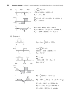
5-13
RO =
7
10
(800) +
5
10
(600) = 860 lbf
RC =
3
10
(800) +
5
10
(600) = 540 lbf
M1 = 860(3)(12) = 30.96(103
) lbf · in
M2 = 30.96(103
) + 60(2)(12)
= 32.40(103
) lbf · in
σmax =
Mmax
Z
⇒ 6 =
32.40
Z
Z = 5.4 in3
y|x=5ft =
F1a[l − (l/2)]
6E Il
l
2
2
+ a2
− 2l
l
2
−
F2l3
48E I
−
1
16
=
800(36)(60)
6(30)(106)I (120)
[602
+ 362
− 1202
] −
600(1203
)
48(30)(106)I
I = 23.69 in4
⇒ I/2 = 11.84 in4
Select two 6 in-8.2 lbf/ft channels; from TableA-7, I = 2(13.1) = 26.2 in4
, Z = 2(4.38) in3
ymax =
23.69
26.2
−
1
16
= −0.0565 in
σmax =
32.40
2(4.38)
= 3.70 kpsi
5-14
I =
π
64
(1.54
) = 0.2485 in4
Superpose beams A-9-6 and A-9-7,
yA =
300(24)(16)
6(30)(106)(0.2485)(40)
(162
+ 242
− 402
)
+
12(16)
24(30)(106)(0.2485)
[2(40)(162
) − 163
− 403
]
yA = −0.1006 in Ans.
y|x=20 =
300(16)(20)
6(30)(106)(0.2485)(40)
[202
+ 162
− 2(40)(20)]
−
5(12)(404)
384(30)(106)(0.2485)
= −0.1043 in Ans.
% difference =
0.1043 − 0.1006
0.1006
(100) = 3.79% Ans.
RC
M1 M2
RO
A
O
B
C
V (lbf)
M
(lbf•in)
800 lbf 600 lbf
3 ft
860
60
O
Ϫ540
2 ft 5 ft
shi20396_ch05.qxd 8/18/03 10:59 AM Page 111

112. 112 Solutions Manual • Instructor’s Solution Manual to Accompany Mechanical Engineering Design
5-15
I =
1
12
3
8
(1.53
) = 0.105 47 in4
From Table A-9-10
yC = −
Fa2
3E I
(l + a)
dyAB
dx
=
Fa
6E Il
(l2
− 3x2
)
Thus,
θA =
Fal2
6E Il
=
Fal
6E I
yD = −θAa = −
Fa2
l
6E I
With both loads,
yD = −
Fa2
l
6E I
−
Fa2
3E I
(l + a)
= −
Fa2
6E I
(3l + 2a) = −
120(102
)
6(30)(106)(0.105 47)
[3(20) + 2(10)]
= −0.050 57 in Ans.
yE =
2Fa(l/2)
6E Il
l2
−
l
2
2
=
3
24
Fal2
E I
=
3
24
120(10)(202
)
(30)(106)(0.105 47)
= 0.018 96 in Ans.
5-16 a = 36 in, l = 72 in, I = 13 in4
, E = 30 Mpsi
y =
F1a2
6E I
(a − 3l) −
F2l3
3E I
=
400(36)2
(36 − 216)
6(30)(106)(13)
−
400(72)3
3(30)(106)(13)
= −0.1675 in Ans.
5-17 I = 2(1.85) = 3.7 in4
Adding the weight of the channels, 2(5)/12 = 0.833 lbf/in,
yA = −
wl4
8E I
−
Fl3
3E I
= −
10.833(484)
8(30)(106)(3.7)
−
220(483)
3(30)(106)(3.7)
= −0.1378 in Ans.
␪A
a
D C
F
B a
EA
shi20396_ch05.qxd 8/18/03 10:59 AM Page 112

113. Chapter 5 113
5-18
I = πd4/64 = π(2)4/64 = 0.7854 in4
Tables A-9-5 and A-9-9
y = −
F2l3
48E I
+
F1a
24E I
(4a2
− 3l2
)
= −
120(40)3
48(30)(106)(0.7854)
+
80(10)(400 − 4800)
24(30)(106)(0.7854)
= −0.0130 in Ans.
5-19
(a) Useful relations
k =
F
y
=
48E I
l3
I =
kl3
48E
=
2400(48)3
48(30)106
= 0.1843 in4
From I = bh3
/12
h = 3
12(0.1843)
b
Form a table. First, Table A-17 gives likely available fractional sizes for b:
81
2, 9, 91
2, 10 in
For h:
1
2
,
9
16
,
5
8
,
11
16
,
3
4
For available b what is necessary h for required I?
(b)
I = 9(0.625)3/12 = 0.1831 in4
k =
48E I
l3
=
48(30)(106
)(0.1831)
483
= 2384 lbf/in
F =
4σ I
cl
=
4(90 000)(0.1831)
(0.625/2)(48)
= 4394 lbf
y =
F
k
=
4394
2384
= 1.84 in Ans.
choose 9"×
5
8
"
Ans.
b
3
12(0.1843)
b
8.5 0.638
9.0 0.626 ←
9.5 0.615
10.0 0.605
shi20396_ch05.qxd 8/18/03 10:59 AM Page 113

114. 114 Solutions Manual • Instructor’s Solution Manual to Accompany Mechanical Engineering Design
5-20
Torque = (600 − 80)(9/2) = 2340 lbf · in
(T2 − T1)
12
2
= T2(1 − 0.125)(6) = 2340
T2 =
2340
6(0.875)
= 446 lbf, T1 = 0.125(446) = 56 lbf
M0 = 12(680) − 33(502) + 48R2 = 0
R2 =
33(502) − 12(680)
48
= 175 lbf
R1 = 680 − 502 + 175 = 353 lbf
We will treat this as two separate problems and then sum the results.
First, consider the 680 lbf load as acting alone.
zO A = −
Fbx
6E Il
(x2
+ b2
− l2
); here b = 36",
x = 12", l = 48", F = 680 lbf
Also,
I =
πd4
64
=
π(1.5)4
64
= 0.2485 in4
zA = −
680(36)(12)(144 + 1296 − 2304)
6(30)(106)(0.2485)(48)
= +0.1182 in
zAC = −
Fa(l − x)
6E Il
(x2
+ a2
− 2lx)
where a = 12" and x = 21 + 12 = 33"
zB = −
680(12)(15)(1089 + 144 − 3168)
6(30)(106)(0.2485)(48)
= +0.1103 in
Next, consider the 502 lbf load as acting alone.
680 lbf
A CBO
R1 ϭ 510 lbf R2 ϭ 170 lbf
12" 21" 15"
z
x
R2 ϭ 175 lbf680 lbf
A C
BO
R1 ϭ 353 lbf 502 lbf
12" 21" 15"
z
x
shi20396_ch05.qxd 8/18/03 10:59 AM Page 114

115. Chapter 5 115
zO B =
Fbx
6E Il
(x2
+ b2
− l2
), where b = 15",
x = 12", l = 48", I = 0.2485 in4
Then, zA =
502(15)(12)(144 + 225 − 2304)
6(30)(106)(0.2485)(48)
= −0.081 44 in
For zB use x = 33"
zB =
502(15)(33)(1089 + 225 − 2304)
6(30)(106)(0.2485)(48)
= −0.1146 in
Therefore, by superposition
zA = +0.1182 − 0.0814 = +0.0368 in Ans.
zB = +0.1103 − 0.1146 = −0.0043 in Ans.
5-21
(a) Calculate torques and moment of inertia
T = (400 − 50)(16/2) = 2800 lbf · in
(8T2 − T2)(10/2) = 2800 ⇒ T2 = 80 lbf, T1 = 8(80) = 640 lbf
I =
π
64
(1.254
) = 0.1198 in4
Due to 720 lbf, flip beamA-9-6 such that yAB → b = 9, x = 0,l = 20, F = −720 lbf
θB =
dy
dx x=0
= −
Fb
6E Il
(3x2
+ b2
− l2
)
= −
−720(9)
6(30)(106)(0.1198)(20)
(0 + 81 − 400) = −4.793(10−3
) rad
yC = −12θB = −0.057 52 in
Due to 450 lbf, use beam A-9-10,
yC = −
Fa2
3E I
(l + a) = −
450(144)(32)
3(30)(106)(0.1198)
= −0.1923 in
450 lbf720 lbf
9" 11" 12"
O
y
A
B
C
RO
RB
A CB
O
R1 R2
12"
502 lbf
21" 15"
z
x
shi20396_ch05.qxd 8/18/03 10:59 AM Page 115

116. 116 Solutions Manual • Instructor’s Solution Manual to Accompany Mechanical Engineering Design
Adding the two deflections,
yC = −0.057 52 − 0.1923 = −0.2498 in Ans.
(b) At O:
Due to 450 lbf:
dy
dx x=0
=
Fa
6E Il
(l2
− 3x2
)
x=0
=
Fal
6E I
θO = −
720(11)(0 + 112
− 400)
6(30)(106)(0.1198)(20)
+
450(12)(20)
6(30)(106)(0.1198)
= 0.010 13 rad = 0.5805◦
At B:
θB = −4.793(10−3
) +
450(12)
6(30)(106)(0.1198)(20)
[202
− 3(202
)]
= −0.014 81 rad = 0.8485◦
I = 0.1198
0.8485◦
0.06◦
= 1.694 in4
d =
64I
π
1/4
=
64(1.694)
π
1/4
= 2.424 in
Use d = 2.5 in Ans.
I =
π
64
(2.54
) = 1.917 in4
yC = −0.2498
0.1198
1.917
= −0.015 61 in Ans.
5-22
(a) l = 36(12) = 432 in
ymax = −
5wl4
384E I
= −
5(5000/12)(432)4
384(30)(106)(5450)
= −1.16 in
The frame is bowed up 1.16 in with respect to the bolsters. It is fabricated upside down
and then inverted. Ans.
(b) The equation in xy-coordinates is for the center sill neutral surface
y =
wx
24E I
(2lx2
− x3
− l3
) Ans.
y
x
l
shi20396_ch05.qxd 8/18/03 10:59 AM Page 116

117. Chapter 5 117
Differentiating this equation and solving for the slope at the left bolster gives
Thus,
dy
dx
=
w
24E I
(6lx2
− 4x3
− l3
)
dy
dx x=0
= −
wl3
24E I
= −
(5000/12)(432)3
24(30)(106)(5450)
= −0.008 57
The slope at the right bolster is 0.00857, so equation at left end is y = −0.008 57x and
at the right end is y = 0.008 57(x − l). Ans.
5-23 From Table A-9-6,
yL =
Fbx
6E Il
(x2
+ b2
− l2
)
yL =
Fb
6E Il
(x3
+ b2
x − l2
x)
dyL
dx
=
Fb
6E Il
(3x2
+ b2
− l2
)
dyL
dx x=0
=
Fb(b2
− l2
)
6E Il
Let ξ =
Fb(b2 − l2)
6E Il
And set I =
πd4
L
64
And solve for dL
dL =
32Fb(b2 − l2)
3π Elξ
1/4
Ans.
For the other end view, observe the figure of Table A-9-6 from the back of the page, noting
that a and b interchange as do x and −x
dR =
32Fa(l2 − a2)
3π Elξ
1/4
Ans.
For a uniform diameter shaft the necessary diameter is the larger of dL and dR.
shi20396_ch05.qxd 8/18/03 10:59 AM Page 117

118. 118 Solutions Manual • Instructor’s Solution Manual to Accompany Mechanical Engineering Design
5-24 Incorporating a design factor into the solution for dL of Prob. 5-23,
d =
32n
3π Elξ
Fb(l2
− b2
)
1/4
= (mm 10−3
)
kN mm3
GPa mm
103
(10−9
)
109(10−3)
1/4
d = 4
32(1.28)(3.5)(150)|(2502 − 1502)|
3π(207)(250)(0.001)
10−12
= 36.4 mm Ans.
5-25 The maximum occurs in the right section. Flip beam A-9-6 and use
y =
Fbx
6E Il
(x2
+ b2
− l2
) where b = 100 mm
dy
dx
=
Fb
6E Il
(3x2
+ b2
− l2
) = 0
Solving for x,
x =
l2 − b2
3
=
2502 − 1002
3
= 132.29 mm from right
y =
3.5(103
)(0.1)(0.132 29)
6(207)(109)(π/64)(0.03644)(0.25)
[0.132 292
+ 0.12
− 0.252
](103
)
= −0.0606 mm Ans.
5-26
x
y
z
F1
a2
b2
b1
a1
F2
3.5 kN
100
250
150
d
The slope at x = 0 due to F1 in the xy plane is
θxy =
F1b1 b2
1 − l2
6E Il
and in the xz plane due to F2 is
θxz =
F2b2 b2
2 − l2
6E Il
For small angles, the slopes add as vectors. Thus
θL = θ2
xy + θ2
xz
1/2
=


F1b1 b2
1 − l2
6E Il
2
+
F2b2 b2
2 − l2
6E Il
2


1/2
shi20396_ch05.qxd 8/18/03 10:59 AM Page 118

119. Chapter 5 119
Designating the slope constraint as ξ, we then have
ξ = |θL| =
1
6E Il
Fi bi b2
i − l2 2 1/2
Setting I = πd4
/64 and solving for d
d =
32
3π Elξ
Fi bi b2
i − l2 2 1/2 1/4
For the LH bearing, E = 30 Mpsi, ξ = 0.001, b1 = 12, b2 = 6, and l = 16. The result is
dL =1.31 in. Using a similar flip beam procedure, we get dR = 1.36 in for the RH bearing.
So use d = 1 3/8 in Ans.
5-27 For the xy plane, use yBC of Table A-9-6
y =
100(4)(16 − 8)
6(30)(106)(16)
[82
+ 42
− 2(16)8] = −1.956(10−4
) in
For the xz plane use yAB
z =
300(6)(8)
6(30)(106)(16)
[82
+ 62
− 162
] = −7.8(10−4
) in
δ = (−1.956j − 7.8k)(10−4
) in
|δ| = 8.04(10−4
) in Ans.
5-28
dL =
32n
3π Elξ
Fi bi b2
i − l2 2 1/2 1/4
=
32(1.5)
3π(29.8)(106)(10)(0.001)
[800(6)(62
− 102
)]2
+ [600(3)(32
− 102
)]2 1/2
1/4
= 1.56 in
dR =
32(1.5)
3π(29.8)(106)(10)(0.001)
[800(4)(102
− 42
)]2
+ [600(7)(102
− 72
)]2 1/2
1/4
= 1.56 in choose d ≥ 1.56 in Ans.
5-29 From Table A-9-8 we have
yL =
MB x
6E Il
(x2
+ 3a2
− 6al + 2l2
)
dyL
dx
=
MB
6E Il
(3x2
+ 3a2
− 6al + 2l2
)
shi20396_ch05.qxd 8/18/03 10:59 AM Page 119

120. 120 Solutions Manual • Instructor’s Solution Manual to Accompany Mechanical Engineering Design
At x = 0, the LH slope is
θL =
dyL
dx
=
MB
6E Il
(3a2
− 6al + 2l2
)
from which
ξ = |θL| =
MB
6E Il
(l2
− 3b2
)
Setting I = πd4
/64 and solving for d
d =
32MB(l2
− 3b2
)
3π Elξ
1/4
For a multiplicity of moments, the slopes add vectorially and
dL =
32
3π Elξ
Mi l2
− 3b2
i
2 1/2 1/4
dR =
32
3π Elξ
Mi 3a2
i − l2 2 1/2 1/4
The greatest slope is at the LH bearing. So
d =
32(1200)[92
− 3(42
)]
3π(30)(106)(9)(0.002)
1/4
= 0.706 in
So use d = 3/4 in Ans.
5-30
6FAC = 18(80)
FAC = 240 lbf
RO = 160 lbf
I =
1
12
(0.25)(23
) = 0.1667 in4
Initially, ignore the stretch of AC. From Table A-9-10
yB1 = −
Fa2
3E I
(l + a) = −
80(122
)
3(10)(106)(0.1667)
(6 + 12) = −0.041 47 in
Stretch of AC: δ =
FL
AE AC
=
240(12)
(π/4)(1/2)2
(10)(106)
= 1.4668(10−3
) in
Due to stretch of AC
By superposition,
yB2 = −3δ = −4.400(10−3
) in
yB = −0.041 47 − 0.0044 = −0.045 87 in Ans.
80 lbfFAC
126
B
RO
shi20396_ch05.qxd 8/18/03 10:59 AM Page 120

121. Chapter 5 121
5-31
θ =
T L
JG
=
(0.1F)(1.5)
(π/32)(0.0124)(79.3)(109)
= 9.292(10−4
)F
Due to twist
δB1 = 0.1(θ) = 9.292(10−5
)F
Due to bending
δB2 =
FL3
3E I
=
F(0.13
)
3(207)(109)(π/64)(0.0124)
= 1.582(10−6
)F
δB = 1.582(10−6
)F + 9.292(10−5
)F = 9.450(10−5
)F
k =
1
9.450(10−5)
= 10.58(103
) N/m = 10.58 kN/m Ans.
5-32
R1 =
Fb
l
R2 =
Fa
l
δ1 =
R1
k1
δ2 =
R2
k2
Spring deflection
yS = −δ1 +
δ1 − δ2
l
x = −
Fb
k1l
+
Fb
k1l2
−
Fa
k2l2
x
yAB =
Fbx
6E Il
(x2
+ b2
− l2
) +
Fx
l2
b
k1
−
a
k2
−
Fb
k1l
Ans.
yBC =
Fa(l − x)
6E Il
(x2
+ a2
− 2lx) +
Fx
l2
b
k1
−
a
k2
−
Fb
k1l
Ans.
5-33 See Prob. 5-32 for deflection due to springs. Replace Fb/l and Fa/l with wl/2
yS = −
wl
2k1
+
wl
2k1l
−
wl
2k2l
x =
wx
2
1
k1
+
1
k2
−
wl
2k1
y =
wx
24E I
(2lx2
− x3
− l3
) +
wx
2
1
k1
+
1
k2
−
wl
2k1
Ans.
F
ba CA B
l
R2
␦2␦1
R1
shi20396_ch05.qxd 8/18/03 10:59 AM Page 121

122. 122 Solutions Manual • Instructor’s Solution Manual to Accompany Mechanical Engineering Design
5-34 Let the load be at x > l/2. The maximum deflection will be in Section AB (Table A-9-10)
yAB =
Fbx
6E Il
(x2
+ b2
− l2
)
dyAB
dx
=
Fb
6E Il
(3x2
+ b2
− l2
) = 0 ⇒ 3x2
+ b2
− l2
= 0
x =
l2 − b2
3
, xmax =
l2
3
= 0.577l Ans.
For x < l/2 xmin = l − 0.577l = 0.423l Ans.
5-35
MO = 50(10)(60) + 600(84)
= 80 400 lbf · in
RO = 50(10) + 600 = 1100 lbf
I = 11.12 in4
from Prob. 5-12
M = −80 400 + 1100x −
4.167x2
2
− 600 x − 84 1
E I
dy
dx
= −80 400x + 550x2
− 0.6944x3
− 300 x − 84 2
+ C1
dy
dx
= 0 at x = 0 І C1 = 0
E I y = −402 00x2
+ 183.33x3
− 0.1736x4
− 100 x − 84 3
+ C2
y = 0 at x = 0 І C2 = 0
yB =
1
30(106)(11.12)
[−40 200(1202
) + 183.33(1203
)
− 0.1736(1204
) − 100(120 − 84)3
]
= −0.9075 in Ans.
5-36 See Prob. 5-13 for reactions: RO = 860 lbf, RC = 540 lbf
M = 860x − 800 x − 36 1
− 600 x − 60 1
E I
dy
dx
= 430x2
− 400 x − 36 2
− 300 x − 60 2
+ C1
E I y = 143.33x3
− 133.33 x − 36 3
− 100 x − 60 3
+ C1x + C2
y = 0 at x = 0 ⇒ C2 = 0
y = 0 at x = 120 in ⇒ C1 = −1.2254(106
) lbf · in2
Substituting C1 and C2 and evaluating at x = 60,
E I y = 30(106
)I −
1
16
= 143.33(603
) − 133.33(60 − 36)3
− 1.2254(106
)(60)
I = 23.68 in4
Agrees with Prob. 5-13. The rest of the solution is the same.
10'
7'
RO
600 lbf50 lbf/ft
MO
O
A
B
shi20396_ch05.qxd 8/18/03 10:59 AM Page 122

123. Chapter 5 123
5-37
I = 0.2485 in4
RO = 12(20) +
24
40
(300) = 420 lbf
M = 420x −
12
2
x2
− 300 x − 16 1
E I
dy
dx
= 210x2
− 2x3
− 150 x − 16 2
+ C1
E I y = 70x3
− 0.5x4
− 50 x − 16 3
+ C1x + C2
y = 0 at x = 0 ⇒ C2 = 0
y = 0 at x = 40 in ⇒ C1 = −6.272(104
) lbf · in2
Substituting for C1 and C2 and evaluating at x = 16,
yA =
1
30(106)(0.2485)
[70(163
) − 0.5(164
) − 6.272(104
)(16)]
= −0.1006 in Ans.
y|x=20 =
1
30(106)(0.2485)
[70(203
) − 0.5(204
) − 50(20 − 16)3
− 6.272(104
)(20)]
= 0.1043 in Ans.
3.7% difference Ans.
5-38
R1 =
w[(l + a)/2][(l − a)/2)]
l
=
w
4l
(l2
− a2
)
R2 =
w
2
(l + a) −
w
4l
(l2
− a2
) =
w
4l
(l + a)2
M =
w
4l
(l2
− a2
)x −
wx2
2
+
w
4l
(l + a)2
x − l 1
E I
dy
dx
=
w
8l
(l2
− a2
)x2
−
w
6
x3
+
w
8l
(l + a)2
x − l 2
+ C1
E I y =
w
24l
(l2
− a2
)x3
−
w
24
x4
+
w
24l
(l + a)2
x − l 3
+ C1x + C2
y = 0 at x = 0 ⇒ C2 = 0
y = 0 at x = l
0 =
w
24l
(l2
− a2
)l3
−
w
24
l4
+ C1l ⇒ C1 =
wa2
l
24
y =
w
24E Il
[(l2
− a2
)x3
− lx4
+ (l + a)2
x − l 3
+ a2
l2
x] Ans.
a
w
l ϩ a
2΂ ΃
l Ϫ a
2
shi20396_ch05.qxd 8/18/03 10:59 AM Page 123

124. 124 Solutions Manual • Instructor’s Solution Manual to Accompany Mechanical Engineering Design
5-39 From Prob. 5-15, RA = RB = 120 lbf, and I = 0.105 47 in4
First half of beam,
M = −120x + 120 x − 10 1
E I
dy
dx
= −60x2
+ 60 x − 10 2
+ C1
dy/dx = 0 at x = 20 in ⇒ 0 = −60(202
) + 60(20 −10)2
+ C1 ⇒ C1 = 1.8(104
) lbf · in2
E I y = −20x3
+ 20 x − 10 3
+ 1.8(104
)x + C2
y = 0 at x = 10 in ⇒ C2 = −1.6(105
) lbf · in3
y|x=0 =
1
30(106)(0.105 47)
(−1.6)(105
)
= −0.050 57 in Ans.
y|x=20 =
1
30(106)(0.105 47)
[−20(203
) + 20(20 − 10)3
+ 1.8(104
)(20) − 1.6(105
)]
= 0.018 96 in Ans.
5-40 From Prob. 5-30, RO = 160 lbf ↓, FAC = 240 lbf I = 0.1667 in4
M = −160x + 240 x − 6 1
E I
dy
dx
= −80x2
+ 120 x − 6 2
+ C1
E I y = −26.67x3
+ 40 x − 6 3
+ C1x + C2
y = 0 at x = 0 ⇒ C2 = 0
yA = −
FL
AE AC
= −
240(12)
(π/4)(1/2)2(10)(106)
= −1.4668(10−3
) in
at x = 6
10(106
)(0.1667)(−1.4668)(10−3
) = −26.67(63
) + C1(6)
C1 = 552.58 lbf · in2
yB =
1
10(106)(0.1667)
[−26.67(183
) + 40(18 − 6)3
+ 552.58(18)]
= −0.045 87 in Ans.
5-41
I1 =
π
64
(1.54
) = 0.2485 in4
I2 =
π
64
(24
) = 0.7854 in4
R1 =
200
2
(12) = 1200 lbf
For 0 ≤ x ≤ 16 in, M = 1200x −
200
2
x − 4 2 x
MրI
shi20396_ch05.qxd 8/18/03 10:59 AM Page 124

125. Chapter 5 125
M
I
=
1200x
I1
− 4800
1
I1
−
1
I2
x − 4 0
− 1200
1
I1
−
1
I2
x − 4 1
−
100
I2
x − 4 2
= 4829x − 13 204 x − 4 0
− 3301.1 x − 4 1
− 127.32 x − 4 2
E
dy
dx
= 2414.5x2
− 13 204 x − 4 1
− 1651 x − 4 2
− 42.44 x − 4 3
+ C1
Boundary Condition:
dy
dx
= 0 at x = 10 in
0 = 2414.5(102
) − 13 204(10 − 4)1
− 1651(10 − 4)2
− 42.44(10 − 4)3
+ C1
C1 = −9.362(104
)
Ey = 804.83x3
− 6602 x − 4 2
− 550.3 x − 4 3
− 10.61 x − 4 4
− 9.362(104
)x + C2
y = 0 at x = 0 ⇒ C2 = 0
For 0 ≤ x ≤ 16 in
y =
1
30(106)
[804.83x3
− 6602 x − 4 2
− 550.3 x − 4 3
− 10.61 x − 4 4
− 9.362(104
)x] Ans.
at x = 10 in
y|x=10 =
1
30(106)
[804.83(103
) − 6602(10 − 4)2
− 550.3(10 − 4)3
− 10.61(10 − 4)4
− 9.362(104
)(10)]
= −0.016 72 in Ans.
5-42 Define δi j as the deflection in the direction of the load at station i due to a unit load at station j.
If U is the potential energy of strain for a body obeying Hooke’s law, apply P1 first. Then
U =
1
2
P1(P1δ11)
When the second load is added, U becomes
U =
1
2
P1(P1δ11) +
1
2
P2(P2 δ22) + P1(P2 δ12)
For loading in the reverse order
U =
1
2
P2(P2 δ22) +
1
2
P1(P1δ11) + P2(P1 δ21)
Since the order of loading is immaterial U = U and
P1 P2δ12 = P2 P1δ21 when P1 = P2, δ12 = δ21
which states that the deflection at station 1 due to a unit load at station 2 is the same as the
deflection at station 2 due to a unit load at 1. δ is sometimes called an influence coefficient.
shi20396_ch05.qxd 8/18/03 10:59 AM Page 125

126. 126 Solutions Manual • Instructor’s Solution Manual to Accompany Mechanical Engineering Design
5-43
(a) From Table A-9-10
yAB =
Fcx(l2
− x2
)
6E Il
δ12 =
y
F x=a
=
ca(l2
− a2
)
6E Il
y2 = Fδ21 = Fδ12 =
Fca(l2
− a2
)
6E Il
Substituting I =
πd4
64
y2 =
400(7)(9)(232
− 92
)(64)
6(30)(106)(π)(2)4(23)
= 0.00347 in Ans.
(b) The slope of the shaft at left bearing at x = 0 is
θ =
Fb(b2 − l2)
6E Il
Viewing the illustration in Section 6 of Table A-9 from the back of the page provides
the correct view of this problem. Noting that a is to be interchanged with b and −x
with x leads to
θ =
Fa(l2 − a2)
6E Il
=
Fa(l2 − a2)(64)
6Eπd4l
θ =
400(9)(232
− 92
)(64)
6(30)(106)(π)(2)4(23)
= 0.000 496 in/in
So y2 = 7θ = 7(0.000 496) = 0.00347 in Ans.
5-44 Place a dummy load Q at the center. Then,
M =
wx
2
(l − x) +
Qx
2
U = 2
l/2
0
M2
dx
2E I
, ymax =
∂U
∂Q Q=0
ymax = 2
l/2
0
2M
2E I
∂M
∂Q
dx
Q=0
ymax =
2
E I
l/2
0
wx
2
(l − x) +
Qx
2
x
2
dx
Q=0
Set Q = 0 and integrate
400 lbf
9"
a
A B
c
21
x
b
7"
23"
y
shi20396_ch05.qxd 8/18/03 10:59 AM Page 126

127. Chapter 5 127
ymax =
w
2E I
lx3
3
−
x4
4
l/2
0
ymax =
5wl4
384E I
Ans.
5-45
I = 2(1.85) = 3.7 in4
Adding weight of channels of 0.833 lbf · in,
M = −Fx −
10.833
2
x2
= −Fx − 5.417x2 ∂M
∂F
= −x
δB =
1
E I
48
0
M
∂M
∂F
dx =
1
E I
48
0
(Fx + 5.417x2
)(x) dx
=
(220/3)(483
) + (5.417/4)(484
)
30(106)(3.7)
= 0.1378 in in direction of 220 lbf
ІyB = −0.1378 in Ans.
5-46
IO B =
1
12
(0.25)(23
) = 0.1667 in4
, AAC =
π
4
1
2
2
= 0.196 35 in2
FAC = 3F,
∂FAC
∂F
= 3
right left
M = −F ¯x M = −2Fx
∂M
∂F
= −¯x
∂M
∂F
= −2x
U =
1
2E I
l
0
M2
dx +
F2
AC LAC
2AAC E
δB =
∂U
∂F
=
1
E I
l
0
M
∂M
∂F
dx +
FAC(∂FAC/∂F)LAC
AAC E
=
1
E I
12
0
−F ¯x(−¯x) d ¯x +
6
0
(−2Fx)(−2x) dx +
3F(3)(12)
AAC E
=
1
E I
F
3
(123
) + 4F
63
3
+
108F
AAC E
=
864F
E I
+
108F
AAC E
=
864(80)
10(106)(0.1667)
+
108(80)
0.196 35(10)(106)
= 0.045 86 in Ans.
FAC ϭ 3F
O
A B
F2F
x
6" 12"
x¯
shi20396_ch05.qxd 8/18/03 10:59 AM Page 127

128. 128 Solutions Manual • Instructor’s Solution Manual to Accompany Mechanical Engineering Design
5-47
Torsion T = 0.1F
∂T
∂F
= 0.1
Bending M = −F ¯x
∂M
∂F
= −¯x
U =
1
2E I
M2
dx +
T2
L
2JG
δB =
∂U
∂F
=
1
E I
M
∂M
∂F
dx +
T(∂T/∂F)L
JG
=
1
E I
0.1
0
−F ¯x(−¯x) d ¯x +
0.1F(0.1)(1.5)
JG
=
F
3E I
(0.13
) +
0.015F
JG
Where
I =
π
64
(0.012)4
= 1.0179(10−9
) m4
J = 2I = 2.0358(10−9
) m4
δB = F
0.001
3(207)(109)(1.0179)(10−9)
+
0.015
2.0358(10−9)(79.3)(109)
= 9.45(10−5
)F
k =
1
9.45(10−5)
= 10.58(103
) N/m = 10.58 kN/m Ans.
5-48 From Prob. 5-41, I1 = 0.2485 in4
, I2 = 0.7854 in4
For a dummy load ↑ Q at the center
0 ≤ x ≤ 10 in M = 1200x −
Q
2
x −
200
2
x − 4 2
,
∂M
∂Q
=
−x
2
y|x=10 =
∂U
∂Q Q=0
=
2
E
1
I1
4
0
(1200x) −
x
2
dx +
1
I2
10
4
[1200x − 100(x − 4)2
] −
x
2
dx
=
2
E
−
200(43
)
I1
−
1.566(105
)
I2
= −
2
30(106)
1.28(104
)
0.2485
+
1.566(105
)
0.7854
= −0.016 73 in Ans.
x
F
shi20396_ch05.qxd 8/18/03 10:59 AM Page 128

129. Chapter 5 129
5-49
AB
M = Fx
∂M
∂F
= x
OA N =
3
5
F
∂N
∂F
=
3
5
T =
4
5
Fa
∂T
∂F
=
4
5
a
M1 =
4
5
F ¯x
∂M1
∂F
=
4
5
¯x
M2 =
3
5
Fa
∂M2
∂F
=
3
5
a
δB =
∂u
∂F
=
1
E I
a
0
Fx(x) dx +
(3/5)F(3/5)l
AE
+
(4/5)Fa(4a/5)l
JG
+
1
E I
l
0
4
5
F ¯x
4
5
¯x d ¯x +
1
E I
l
0
3
5
Fa
3
5
a d ¯x
=
Fa3
3E I
+
9
25
Fl
AE
+
16
25
Fa2
l
JG
+
16
75
Fl3
E I
+
9
25
Fa2
l
E I
I =
π
64
d4
, J = 2I, A =
π
4
d2
δB =
64Fa3
3Eπd4
+
9
25
4Fl
πd2 E
+
16
25
32Fa2
l
πd4G
+
16
75
64Fl3
Eπd4
+
9
25
64Fa2
l
Eπd4
=
4F
75π Ed4
400a3
+ 27ld2
+ 384a2
l
E
G
+ 256l3
+ 432a2
l Ans.
a
O
B
A
F
3
5
F
4
5
a
B
x
A
F
3
5
F
4
5
O
l
l
A
F
3
5
Fa
3
5
Fa
4
5
F
4
5
x
shi20396_ch05.qxd 8/18/03 10:59 AM Page 129

130. 130 Solutions Manual • Instructor’s Solution Manual to Accompany Mechanical Engineering Design
5-50 The force applied to the copper and steel wire assembly is Fc + Fs = 250 lbf
Since δc = δs
FcL
3(π/4)(0.0801)2(17.2)(106)
=
Fs L
(π/4)(0.0625)2(30)(106)
Fc = 2.825Fs
∴ 3.825Fs = 250 ⇒ Fs = 65.36 lbf, Fc = 2.825Fs = 184.64 lbf
σc =
184.64
3(π/4)(0.0801)2
= 12 200 psi = 12.2 kpsi Ans.
σs =
65.36
(π/4)(0.06252)
= 21 300 psi = 21.3 kpsi Ans.
5-51
(a) Bolt stress σb = 0.9(85) = 76.5 kpsi Ans.
Bolt force Fb = 6(76.5)
π
4
(0.3752
) = 50.69 kips
Cylinder stress σc = −
Fb
Ac
= −
50.69
(π/4)(4.52 − 42)
= −15.19 kpsi Ans.
(b) Force from pressure
P =
π D2
4
p =
π(42
)
4
(600) = 7540 lbf = 7.54 kip
Fx = 0
Pb + Pc = 7.54 (1)
Since δc = δb ,
PcL
(π/4)(4.52 − 42)E
=
PbL
6(π/4)(0.3752)E
Pc = 5.037Pb (2)
Substituting into Eq. (1)
6.037Pb = 7.54 ⇒ Pb = 1.249 kip; and from Eq (2), Pc = 6.291 kip
Using the results of (a) above, the total bolt and cylinder stresses are
σb = 76.5 +
1.249
6(π/4)(0.3752)
= 78.4 kpsi Ans.
σc = −15.19 +
6.291
(π/4)(4.52 − 42)
= −13.3 kpsi Ans.
6 bolts
50.69 Ϫ Pc
50.69 ϩ Pb
x
P ϭ 7.54 kip
shi20396_ch05.qxd 8/18/03 10:59 AM Page 130

131. Chapter 5 131
5-52
T = Tc + Ts and θc = θs
Also,
TcL
(G J)c
=
Ts L
(G J)s
Tc =
(G J)c
(G J)s
Ts
Substituting into equation for T ,
T = 1 +
(G J)c
(G J)s
Ts
%Ts =
Ts
T
=
(G J)s
(G J)s + (G J)c
Ans.
5-53
RO + RB = W (1)
δO A = δAB (2)
20RO
AE
=
30RB
AE
, RO =
3
2
RB
3
2
RB + RB = 800
RB =
1600
5
= 320 lbf Ans.
RO = 800 − 320 = 480 lbf Ans.
σO = −
480
1
= −480 psi Ans.
σB = +
320
1
= 320 psi Ans.
5-54 Since θO A = θAB
TO A(4)
G J
=
TAB(6)
G J
, TO A =
3
2
TAB
Also TO A + TAB = T
TAB
3
2
+ 1 = T, TAB =
T
2.5
Ans.
TO A =
3
2
TAB =
3T
5
Ans.
RB
W ϭ 800 lbf
30"
20"
RO
A
B
O
shi20396_ch05.qxd 8/18/03 10:59 AM Page 131

132. 132 Solutions Manual • Instructor’s Solution Manual to Accompany Mechanical Engineering Design
5-55
F1 = F2 ⇒
T1
r1
=
T2
r2
⇒
T1
1.25
=
T2
3
T2 =
3
1.25
T1
∴ θ1 +
3
1.25
θ2 =
4π
180
rad
T1(48)
(π/32)(7/8)4(11.5)(106)
+
3
1.25
(3/1.25)T1(48)
(π/32)(1.25)4(11.5)(106)
=
4π
180
T1 = 403.9 lbf · in
T2 =
3
1.25
T1 = 969.4 lbf · in
τ1 =
16T1
πd3
=
16(403.9)
π(7/8)3
= 3071 psi Ans.
τ2 =
16(969.4)
π(1.25)3
= 2528 psi Ans.
5-56
(1) Arbitrarily, choose RC as redundant reaction
(2) Fx = 0, 10(103
) − 5(103
) − RO − RC = 0
RO + RC = 5(103
) lbf
(3) δC =
[10(103
) − 5(103
) − RC]20
AE
−
[5(103
) + RC]
AE
(10) −
RC(15)
AE
= 0
−45RC + 5(104
) = 0 ⇒ RC = 1111 lbf Ans.
RO = 5000 − 1111 = 3889 lbf Ans.
5-57
(1) Choose RB as redundant reaction
(2) RB + RC = wl (a) RB(l − a) −
wl2
2
+ MC = 0 (b)
RB
A
x
w
RC
CB
MC
a
l
10 kip 5 kip
FA FB RCRO x
shi20396_ch05.qxd 8/18/03 10:59 AM Page 132

133. Chapter 5 133
(3) yB =
RB(l − a)3
3E I
+
w(l − a)2
24E I
[4l(l − a) − (l − a)2
− 6l2
] = 0
RB =
w
8(l − a)
[6l2
− 4l(l − a) + (l − a)2
]
=
w
8(l − a)
(3l2
+ 2al + a2
) Ans.
Substituting,
Eq. (a) RC = wl − RB =
w
8(l − a)
(5l2
− 10al − a2
) Ans.
Eq. (b) MC =
wl2
2
− RB(l − a) =
w
8
(l2
− 2al − a2
) Ans.
5-58
M = −
wx2
2
+ RB x − a 1
,
∂M
∂ RB
= x − a 1
∂U
∂ RB
=
1
E I
l
0
M
∂M
∂ RB
dx
=
1
E I
a
0
−wx2
2
(0) dx +
1
E I
l
a
−wx2
2
+ RB(x − a) (x − a) dx = 0
−
w
2
1
4
(l4
− a4
) −
a
3
(l3
− a3
) +
RB
3
(l − a)3
− (a − a)3
= 0
RB =
w
(l − a)3
[3(L4
− a4
) − 4a(l3
− a3
)] =
w
8(l − a)
(3l2
+ 2al + a2
) Ans.
RC = wl − RB =
w
8(l − a)
(5l2
− 10al − a2
) Ans.
MC =
wl2
2
− RB(l − a) =
w
8
(l2
− 2al − a2
) Ans.
5-59
A =
π
4
(0.0122
) = 1.131(10−4
) m2
(1) RA + FBE + FDF = 20 kN (a)
MA = 3FDF − 2(20) + FBE = 0
FBE + 3FDF = 40 kN (b)
FBE FDF
D
C
20 kN
500500 500
B
A
RA
RB
A
a B C
RC
MC
x
w
shi20396_ch05.qxd 8/18/03 10:59 AM Page 133

134. 134 Solutions Manual • Instructor’s Solution Manual to Accompany Mechanical Engineering Design
(2) M = RAx + FBE x − 0.5 1
− 20(103
) x − 1 1
E I
dy
dx
= RA
x2
2
+
FBE
2
x − 0.5 2
− 10(103
) x − 1 2
+ C1
E I y = RA
x3
6
+
FBE
6
x − 0.5 3
−
10
3
(103
) x − 1 3
+ C1x + C2
(3) y = 0 at x = 0 І C2 = 0
yB = −
Fl
AE BE
= −
FBE(1)
1.131(10−4)209(109)
= −4.2305(10−8
)FBE
Substituting and evaluating at x = 0.5 m
E I yB = 209(109
)(8)(10−7
)(−4.2305)(10−8
)FBE = RA
0.53
6
+ C1(0.5)
2.0833(10−2
)RA + 7.0734(10−3
)FBE + 0.5C1 = 0 (c)
yD = −
Fl
AE DF
= −
FDF(1)
1.131(10−4)(209)(109)
= −4.2305(10−8
)FDF
Substituting and evaluating at x = 1.5 m
E I yD =−7.0734(10−3
)FDF = RA
1.53
6
+
FBE
6
(1.5 − 0.5)3
−
10
3
(103
)(1.5 − 1)3
+1.5C1
0.5625RA + 0.166 67FBE + 7.0734(10−3
)FDF + 1.5C1 = 416.67 (d)




1 1 1 0
0 1 3 0
2.0833(10−2
) 7.0734(10−3
) 0 0.5
0.5625 0.166 67 7.0734(10−3
) 1.5







RA
FBE
FDF
C1



=



20 000
40 000
0
416.67



Solve simultaneously or use software
RA = −3885 N, FBE = 15 830 N, FDF = 8058 N, C1 = −62.045 N · m2
σBE =
15 830
(π/4)(122)
= 140 MPa Ans., σDF =
8058
(π/4)(122)
= 71.2 MPa Ans.
E I = 209(109
)(8)(10−7
) = 167.2(103
) N · m2
y =
1
167.2(103)
−
3885
6
x3
+
15 830
6
x − 0.5 3
−
10
3
(103
) x − 1 3
− 62.045x
B: x = 0.5 m, yB = −6.70(10−4
) m = −0.670 mm Ans.
C: x = 1 m, yC =
1
167.2(103)
−
3885
6
(13
) +
15 830
6
(1 − 0.5)3
− 62.045(1)
= −2.27(10−3
) m = −2.27 mm Ans.
D: x = 1.5, yD =
1
167.2(103)
−
3885
6
(1.53
) +
15 830
6
(1.5 − 0.5)3
−
10
3
(103
)(1.5 − 1)3
− 62.045(1.5)
= −3.39(10−4
) m = −0.339 mm Ans.
shi20396_ch05.qxd 8/18/03 10:59 AM Page 134

135. Chapter 5 135
5-60
E I = 30(106
)(0.050) = 1.5(106
) lbf · in2
(1) RC + FBE − FFD = 500 (a)
3RC + 6FBE = 9(500) = 4500 (b)
(2) M = −500x + FBE x − 3 1
+ RC x − 6 1
E I
dy
dx
= −250x2
+
FBE
2
x − 3 2
+
RC
2
x − 6 2
+ C1
E I y = −
250
3
x3
+
FBE
6
x − 3 3
+
RC
6
x − 6 3
+ C1x + C2
yB =
Fl
AE BE
= −
FBE(2)
(π/4)(5/16)2(30)(106)
= −8.692(10−7
)FBE
Substituting and evaluating at x = 3 in
E I yB = 1.5(106
)[−8.692(10−7
)FBE] = −
250
3
(33
) + 3C1 + C2
1.3038FBE + 3C1 + C2 = 2250 (c)
Since y = 0 at x = 6 in
E I y|=0 = −
250
3
(63
) +
FBE
6
(6 − 3)3
+ 6C1 + C2
4.5FBE + 6C1 + C2 = 1.8(104
) (d)
yD =
Fl
AE DF
=
FDF(2.5)
(π/4)(5/16)2(30)(106)
= 1.0865(10−6
)FDF
Substituting and evaluating at x = 9 in
E I yD = 1.5(106
)[1.0865(10−6
)FDF] = −
250
3
(93
) +
FBE
6
(9 − 3)3
+
RC
6
(9 − 6)3
+ 9C1 + C2
4.5RC + 36FBE − 1.6297FDF + 9C1 + C2 = 6.075(104
) (e)






1 1 −1 0 0
3 6 0 0 0
0 1.3038 0 3 1
0 4.5 0 6 1
4.5 36 −1.6297 9 1









RC
FBE
FDF
C1
C2



=



500
4500
2250
1.8(104
)
6.075(104
)



RC = −590.4 lbf, FBE = 1045.2 lbf, FDF = −45.2 lbf
C1 = 4136.4 lbf · in2
, C2 = −11 522 lbf · in3
FBE
A B
C D
FFDRC
3"3"
500 lbf
y
3"
x
shi20396_ch05.qxd 8/18/03 10:59 AM Page 135

136. 136 Solutions Manual • Instructor’s Solution Manual to Accompany Mechanical Engineering Design
σBE =
1045.2
(π/4)(5/16)2
= 13 627 psi = 13.6 kpsi Ans.
σDF = −
45.2
(π/4)(5/16)2
= −589 psi Ans.
yA =
1
1.5(106)
(−11 522) = −0.007 68 in Ans.
yB =
1
1.5(106)
−
250
3
(33
) + 4136.4(3) − 11 522 = −0.000 909 in Ans.
yD =
1
1.5(106)
−
250
3
(93
) +
1045.2
6
(9 − 3)3
+
−590.4
6
(9 − 6)3
+ 4136.4(9) − 11 522
= −4.93(10−5
) in Ans.
5-61
M = −P R sin θ + QR(1 − cos θ)
∂M
∂Q
= R(1 − cos θ)
δQ =
∂U
∂Q Q=0
=
1
E I
π
0
(−P R sin θ)R(1 − cos θ)R dθ = −2
P R3
E I
Deflection is upward and equals 2(P R3
/E I) Ans.
5-62 Equation (4-34) becomes
U = 2
π
0
M2
R dθ
2E I
R/h > 10
where M = F R(1 − cos θ) and
∂M
∂F
= R(1 − cos θ)
δ =
∂U
∂F
=
2
E I
π
0
M
∂M
∂F
R dθ
=
2
E I
π
0
F R3
(1 − cos θ)2
dθ
=
3π F R3
E I
F
Q (dummy load)
␪
shi20396_ch05.qxd 8/18/03 10:59 AM Page 136

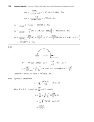
137. Chapter 5 137
Since I = bh3
/12 = 4(6)3
/12 = 72 mm4
and R = 81/2 = 40.5 mm, we have
δ =
3π(40.5)3
F
131(72)
= 66.4F mm Ans.
where F is in kN.
5-63
M = −Px,
∂M
∂ P
= −x 0 ≤ x ≤ l
M = Pl + P R(1 − cos θ),
∂M
∂ P
= l + R(1 − cos θ) 0 ≤ θ ≤ l
δP =
1
E I
l
0
−Px(−x) dx +
π/2
0
P[l + R(1 − cos θ)]2
R dθ
=
P
12E I
{4l3
+ 3R[2πl2
+ 4(π − 2)l R + (3π − 8)R2
]} Ans.
5-64 A: Dummy load Q is applied at A. Bending in AB due only to Q which is zero.
M = P R sin θ + QR(1 + sin θ),
∂M
∂Q
= R(1 + sin θ) 0 ≤ θ ≤
π
2
(δA)V =
∂U
∂Q Q=0
=
1
E I
π/2
0
(P R sin θ)[R(1 + sin θ)]R dθ
=
P R3
E I
−cos θ +
θ
2
−
sin 2θ
4
π/2
0
=
P R3
E I
1 +
π
4
=
π + 4
4
P R3
E I
Ans.
P
Q
B
A
C
␪
P
x
l
R
␪
shi20396_ch05.qxd 8/18/03 10:59 AM Page 137

138. 138 Solutions Manual • Instructor’s Solution Manual to Accompany Mechanical Engineering Design
B: M = P R sin θ,
∂M
∂ P
= R sin θ
(δB)V =
∂U
∂ P
=
1
E I
π/2
0
(P R sin θ)(R sin θ)R dθ
=
π
4
P R3
E I
Ans.
5-65
M = P R sin θ,
∂M
∂ P
= R sin θ 0 < θ <
π
2
T = P R(1 − cos θ),
∂T
∂ P
= R(1 − cos θ)
(δA)y = −
∂U
∂ P
= −
1
E I
π/2
0
P(R sin θ)2
R dθ +
1
G J
π/2
0
P[R(1 − cos θ)]2
R dθ
Integrating and substituting J = 2I and G = E/[2(1 + ν)]
(δA)y = −
P R3
E I
π
4
+ (1 + ν)
3π
4
− 2 = −[4π − 8 + (3π − 8)ν]
P R3
4E I
= −[4π − 8 + (3π − 8)(0.29)]
(200)(100)3
4(200)(103)(π/64)(5)4
= −40.6 mm
5-66 Consider the horizontal reaction, to be applied at B, subject to the constraint (δB)H = 0.
(a) (δB)H =
∂U
∂ H
= 0
Due to symmetry, consider half of the structure. P does not deflect horizontally.
P
A
B H
R
P
2
␪
A
R
z
x
y
M
T
200 N
␪
200 N
shi20396_ch05.qxd 8/18/03 10:59 AM Page 138

139. Chapter 5 139
M =
P R
2
(1 − cos θ) − H R sin θ,
∂M
∂ H
= −R sin θ, 0 < θ <
π
2
∂U
∂ H
=
1
E I
π/2
0
P R
2
(1 − cos θ) − H R sin θ (−R sin θ)R dθ = 0
−
P
2
+
P
4
+ H
π
4
= 0 ⇒ H =
P
π
Ans.
Reaction at A is the same where H goes to the left
(b) For 0 < θ <
π
2
, M =
P R
2
(1 − cos θ) −
P R
π
sin θ
M =
P R
2π
[π(1 − cos θ) − 2 sin θ] Ans.
Due to symmetry, the solution for the left side is identical.
(c)
∂M
∂ P
=
R
2π
[π(1 − cos θ) − 2 sin θ]
δP =
∂U
∂ P
=
2
E I
π/2
0
P R2
4π2
[π(1 − cos θ) − 2 sin θ]2
R dθ
=
P R3
2π2 E I
π/2
0
(π2
+ π2
cos2
θ + 4 sin2
θ − 2π2
cos θ
− 4π sin θ + 4π sin θ cos θ) dθ
=
P R3
2π2 E I
π2 π
2
+ π2 π
4
+ 4
π
4
− 2π2
− 4π + 2π
=
(3π2
− 8π − 4)
8π
P R3
E I
Ans.
5-67 Must use Eq. (5-34)
A = 80(60) − 40(60) = 2400 mm2
R =
(25 + 40)(80)(60) − (25 + 20 + 30)(40)(60)
2400
= 55 mm
Section is equivalent to the “T” section of Table 4-5
rn =
60(20) + 20(60)
60 ln[(25 + 20)/25] + 20 ln[(80 + 25)/(25 + 20)]
= 45.9654 mm
e = R − rn = 9.035 mm
Iz =
1
12
(60)(203
) + 60(20)(30 − 10)2
+ 2
1
12
(10)(603
) + 10(60)(50 − 30)2
= 1.36(106
) mm4
y
z
30 mm
50 mm
Straight section
shi20396_ch05.qxd 8/18/03 10:59 AM Page 139

140. 140 Solutions Manual • Instructor’s Solution Manual to Accompany Mechanical Engineering Design
For 0 ≤ x ≤ 100 mm
M = −Fx,
∂M
∂F
= −x; V = F,
∂V
∂F
= 1
For θ ≤ π/2
Fr = F cos θ,
∂Fr
∂F
= cos θ; Fθ = F sin θ,
∂Fθ
∂F
= sin θ
M = F(100 + 55 sin θ),
∂M
∂F
= (100 + 55 sin θ)
Use Eq. (5-34), integrate from 0 to π/2, double the results and add straight part
δ =
2
E
1
I
100
0
Fx2
dx +
100
0
(1)F(1) dx
2400(G/E)
+
π/2
0
F
(100 + 55 sin θ)2
2400(9.035)
dθ
+
π/2
0
F sin2
θ(55)
2400
dθ −
π/2
0
F(100 + 55 sin θ)
2400
sin θdθ
−
π/2
0
F sin θ(100 + 55 sin θ)
2400
dθ +
π/2
0
(1)F cos2
θ(55)
2400(G/E)
dθ
Substitute
I = 1.36(103
) mm2
, F = 30(103
) N, E = 207(103
) N/mm2
, G = 79(103
) N/mm2
δ =
2
207(103)
30(103
)
1003
3(1.36)(106)
+
207
79
100
2400
+
2.908(104
)
2400(9.035)
+
55
2400
π
4
−
2
2400
(143.197) +
207
79
55
2400
π
4
= 0.476 mm Ans.
5-68
M = F R sin θ − QR(1 − cos θ),
∂M
∂Q
= −R(1 − cos θ)
Fθ = Q cos θ + F sin θ,
∂Fθ
∂Q
= cos θ
∂
∂Q
(M Fθ ) = [F R sin θ − QR(1 − cos θ)] cos θ
+ [−R(1 − cos θ)][Q cos θ + F sin θ]
Fr = F cos θ − Q sin θ,
∂Fr
∂Q
= −sin θ
Q
F
M
R
Fr
F␪
␪
F
F␪Fr
M
␪
100 mm
x
shi20396_ch05.qxd 8/18/03 10:59 AM Page 140

141. Chapter 5 141
From Eq. (5-34)
δ =
∂U
∂Q Q=0
=
1
AeE
π
0
(F R sin θ)[−R(1 − cos θ)] dθ +
R
AE
π
0
F sin θ cos θdθ
−
1
AE
π
0
[F R sin θ cos θ − F R sin θ(1 − cos θ)] dθ
+
C R
AG
π
0
−F cos θ sin θdθ
= −
2F R2
AeE
+ 0 +
2F R
AE
+ 0 = −
R
e
− 1
2F R
AE
Ans.
5-69 The cross section at A does not rotate, thus for a single quadrant we have
∂U
∂MA
= 0
The bending moment at an angle θ to the x axis is
M = MA −
F
2
(R − x) = MA −
F R
2
(1 − cos θ) (1)
because x = R cos θ. Next,
U =
M2
2E I
ds =
π/2
0
M2
2E I
R dθ
since ds = R dθ. Then
∂U
∂MA
=
R
E I
π/2
0
M
∂M
∂MA
dθ = 0
But ∂M/∂MA = 1. Therefore
π/2
0
M dθ =
π/2
0
MA −
F R
2
(1 − cos θ) dθ = 0
Since this term is zero, we have
MA =
F R
2
1 −
2
π
Substituting into Eq. (1)
M =
F R
2
cos θ −
2
π
The maximum occurs at B where θ = π/2. It is
MB = −
F R
π
Ans.
shi20396_ch05.qxd 8/18/03 10:59 AM Page 141

142. 142 Solutions Manual • Instructor’s Solution Manual to Accompany Mechanical Engineering Design
5-70 For one quadrant
M =
F R
2
cos θ −
2
π
;
∂M
∂F
=
R
2
cos θ −
2
π
δ =
∂U
∂F
= 4
π/2
0
M
E I
∂M
∂F
R dθ
=
F R3
E I
π/2
0
cos θ −
2
π
2
dθ
=
F R3
E I
π
4
−
2
π
Ans.
5-71
Pcr =
Cπ2
E I
l2
I =
π
64
(D4
− d4
) =
π D4
64
(1 − K4
)
Pcr =
Cπ2
E
l2
π D4
64
(1 − K4
)
D =
64Pcr l2
π3C E(1 − K4)
1/4
Ans.
5-72
A =
π
4
D2
(1 − K2
), I =
π
64
D4
(1 − K4
) =
π
64
D4
(1 − K2
)(1 + K2
),
k2
=
I
A
=
D2
16
(1 + K2
)
From Eq. (5-50)
Pcr
(π/4)D2(1 − K2)
= Sy −
S2
y l2
4π2k2C E
= Sy −
S2
y l2
4π2(D2/16)(1 + K2)C E
4Pcr = π D2
(1 − K2
)Sy −
4S2
y l2
π D2
(1 − K2
)
π2 D2(1 + K2)C E
π D2
(1 − K2
)Sy = 4Pcr +
4S2
y l2
(1 − K2
)
π(1 + K2)C E
D =
4Pcr
πSy(1 − K2)
+
4S2
y l2
(1 − K2
)
π(1 + K2)C Eπ(1 − K2)Sy
1/2
= 2
Pcr
πSy(1 − K2)
+
Sy l2
π2C E(1 + K2)
1/2
Ans.
shi20396_ch05.qxd 8/18/03 10:59 AM Page 142

143. Chapter 5 143
5-73 (a)
+ MA = 0, 2.5(180) −
3
√
32 + 1.752
FBO(1.75) = 0 ⇒ FBO = 297.7 lbf
Using nd = 5, design for Fcr = nd FBO = 5(297.7) = 1488 lbf, l = 32 + 1.752 =
3.473 ft, Sy = 24 kpsi
In plane: k = 0.2887h = 0.2887", C = 1.0
Try 1" × 1/2" section
l
k
=
3.473(12)
0.2887
= 144.4
l
k 1
=
2π2
(1)(30)(106
)
24(103)
1/2
= 157.1
Since (l/k)1 > (l/k) use Johnson formula
Pcr = (1)
1
2
24(103
) −
24(103
)
2π
144.4
2
1
1(30)(106)
= 6930 lbf
Try 1" × 1/4": Pcr = 3465 lbf
Out of plane: k = 0.2887(0.5) = 0.1444 in, C = 1.2
l
k
=
3.473(12)
0.1444
= 289
Since (l/k)1 < (l/k) use Euler equation
Pcr = 1(0.5)
1.2(π2
)(30)(106
)
2892
= 2127 lbf
1/4" increases l/k by 2,
l
k
2
by 4, and A by 1/2
Try 1" × 3/8": k = 0.2887(0.375) = 0.1083 in
l
k
= 385, Pcr = 1(0.375)
1.2(π2
)(30)(106
)
3852
= 899 lbf (too low)
Use 1" × 1/2" Ans.
(b) σb = −
P
πdl
= −
298
π(0.5)(0.5)
= −379 psi No, bearing stress is not significant.
5-74 This is a design problem with no one distinct solution.
5-75
F = 800
π
4
(32
) = 5655 lbf, Sy = 37.5 kpsi
Pcr = nd F = 3(5655) = 17 000 lbf
shi20396_ch05.qxd 8/18/03 10:59 AM Page 143

144. 144 Solutions Manual • Instructor’s Solution Manual to Accompany Mechanical Engineering Design
(a) Assume Euler with C = 1
I =
π
64
d4
=
Pcr l2
Cπ2 E
⇒ d =
64Pcr l2
π3C E
1/4
=
64(17)(103
)(602
)
π3(1)(30)(106)
1/4
= 1.433 in
Use d = 1.5 in; k = d/4 = 0.375
l
k
=
60
0.375
= 160
l
k 1
=
2π2
(1)(30)(106
)
37.5(103)
1/2
= 126 ∴ use Euler
Pcr =
π2
(30)(106
)(π/64)(1.54
)
602
= 20 440 lbf
d = 1.5 in is satisfactory. Ans.
(b) d =
64(17)(103
)(182
)
π3(1)(30)(106)
1/4
= 0.785 in, so use 0.875 in
k =
0.875
4
= 0.2188 in
l/k =
18
0.2188
= 82.3 try Johnson
Pcr =
π
4
(0.8752
) 37.5(103
) −
37.5(103
)
2π
82.3
2
1
1(30)(106)
= 17 714 lbf
Use d = 0.875 in Ans.
(c) n(a) =
20 440
5655
= 3.61 Ans.
n(b) =
17 714
5655
= 3.13 Ans.
5-76
4F sin θ = 3920
F =
3920
4 sin θ
In range of operation, F is maximum when θ = 15◦
Fmax =
3920
4 sin 15
= 3786 N per bar
Pcr = nd Fmax = 2.5(3786) = 9465 N
l = 300 mm, h = 25 mm
␪ ␪
W ϭ 9.8(400) ϭ 3920 N
2F
2 bars
2F
shi20396_ch05.qxd 8/18/03 10:59 AM Page 144

145. Chapter 5 145
Try b = 5 mm: out of plane k = (5/
√
12) = 1.443 mm
l
k
=
300
1.443
= 207.8
l
k 1
=
(2π2
)(1.4)(207)(109
)
380(106)
1/2
= 123 ∴ use Euler
Pcr = (25)(5)
(1.4π2
)(207)(103
)
(207.8)2
= 8280 N
Try: 5.5 mm: k = 5.5/
√
12 = 1.588 mm
l
k
=
300
1.588
= 189
Pcr = 25(5.5)
(1.4π2
)(207)(103
)
1892
= 11 010 N
Use 25 × 5.5 mm bars Ans. The factor of safety is thus
n =
11 010
3786
= 2.91 Ans.
5-77 F = 0 = 2000 + 10 000 − P ⇒ P = 12 000 lbf Ans.
MA = 12 000
5.68
2
− 10 000(5.68) + M = 0
M = 22 720 lbf · in
e =
M
P
=
22
12
720
000
= 1.893 in Ans.
From Table A-8, A = 4.271 in2
, I = 7.090 in4
k2
=
I
A
=
7.090
4.271
= 1.66 in2
σc = −
12 000
4.271
1 +
1.893(2)
1.66
= −9218 psi Ans.
σt = −
12 000
4.271
1 −
1.893(2)
1.66
= 3598 psi
5-78 This is a design problem so the solutions will differ.
3598 ␴
Ϫ9218
PA C
M
2000 10,000
shi20396_ch05.qxd 8/18/03 10:59 AM Page 145

146. 146 Solutions Manual • Instructor’s Solution Manual to Accompany Mechanical Engineering Design
5-79 For free fall with y ≤ h
Fy − m ¨y = 0
mg − m ¨y = 0, so ¨y = g
Using y = a + bt + ct2
, we have at t = 0, y = 0, and ˙y = 0, and so a = 0, b = 0, and
c = g/2. Thus
y =
1
2
gt2
and ˙y = gt for y ≤ h
At impact, y = h, t = (2h/g)1/2
, and v0 = (2gh)1/2
After contact, the differential equatioin (D.E.) is
mg − k(y − h) − m ¨y = 0 for y > h
Now let x = y − h; then ˙x = ˙y and ¨x = ¨y. So the D.E. is ¨x + (k/m)x = g with solution
ω = (k/m)1/2
and
x = A cos ωt + B sin ωt +
mg
k
At contact, t = 0, x = 0, and ˙x = v0 . Evaluating A and B then yields
x = −
mg
k
cos ωt +
v0
ω
sin ωt +
mg
k
or
y = −
W
k
cos ωt +
v0
ω
sin ωt +
W
k
+ h
and
˙y =
Wω
k
sin ωt + v0 cos ωt
To find ymax set ˙y = 0. Solving gives
tan ωt = −
v0k
Wω
or (ωt )* = tan−1
−
v0k
Wω
The first value of (ωt )* is a minimum and negative. So add π radians to it to find the
maximum.
Numerical example: h = 1 in, W = 30 lbf, k = 100 lbf/in. Then
ω = (k/m)1/2
= [100(386)/30]1/2
= 35.87 rad/s
W/k = 30/100 = 0.3
v0 = (2gh)1/2
= [2(386)(1)]1/2
= 27.78 in/s
Then
y = −0.3 cos 35.87t +
27.78
35.87
sin 35.87t + 0.3 + 1
mg
y
k(y Ϫ h)
mg
y
shi20396_ch05.qxd 8/18/03 10:59 AM Page 146

147. Chapter 5 147
For ymax
tan ωt = −
v0k
Wω
= −
27.78(100)
30(35.87)
= −2.58
(ωt )* = −1.20 rad (minimum)
(ωt )* = −1.20 + π = 1.940 (maximum)
Thent * = 1.940/35.87 = 0.0541 s. This means that the spring bottoms out at t * seconds.
Then (ωt )* = 35.87(0.0541) = 1.94 rad
So ymax = −0.3 cos 1.94 +
27.78
35.87
sin 1.94 + 0.3 + 1 = 2.130 in Ans.
The maximum spring force is Fmax = k(ymax − h) = 100(2.130 − 1) = 113 lbf Ans.
The action is illustrated by the graph below. Applications: Impact, such as a dropped
package or a pogo stick with a passive rider. The idea has also been used for a one-legged
robotic walking machine.
5-80 Choose t = 0 at the instant of impact. At this instant, v1 = (2gh)1/2
. Using momentum,
m1v1 = m2v2 . Thus
W1
g
(2gh)1/2
=
W1 + W2
g
v2
v2 =
W1(2gh)1/2
W1 + W2
Therefore at t = 0, y = 0, and ˙y = v2
Let W = W1 + W2
Because the spring force at y = 0 includes a reaction to W2, the D.E. is
W
g
¨y = −ky + W1
With ω = (kg/W)1/2
the solution is
y = A cos ωt + B sin ωt + W1/k
˙y = −Aω sin ωt + Bω cos ωt
At t = 0, y = 0 ⇒ A = −W1/k
At t = 0, ˙y = v2 ⇒ v2 = Bω
W1ky
y
W1 ϩ W2
Time of
release
Ϫ0.05 Ϫ0.01
2
0
1 0.01 0.05 Time tЈ
Speeds agree
Inflection point of trig curve
(The maximum speed about
this point is 29.8 in/s.)
Equilibrium,
rest deflection
During
contact
Free fall
ymax
y
shi20396_ch05.qxd 8/18/03 10:59 AM Page 147

148. 148 Solutions Manual • Instructor’s Solution Manual to Accompany Mechanical Engineering Design
Then
B =
v2
ω
=
W1(2gh)1/2
(W1 + W2)[kg/(W1 + W2)]1/2
We now have
y = −
W1
k
cos ωt + W1
2h
k(W1 + W2)
1/2
sin ωt +
W1
k
Transforming gives
y =
W1
k
2hk
W1 + W2
+ 1
1/2
cos(ωt − φ) +
W1
k
where φ is a phase angle. The maximum deflection of W2 and the maximum spring force
are thus
ymax =
W1
k
2hk
W1 + W2
+ 1
1/2
+
W1
k
Ans.
Fmax = kymax + W2 = W1
2hk
W1 + W2
+ 1
1/2
+ W1 + W2 Ans.
5-81 Assume x > y to get a free-body diagram.
Then
W
g
¨y = k1(x − y) − k2y
A particular solution for x = a is
y =
k1a
k1 + k2
Then the complementary plus the particular solution is
y = A cos ωt + B sin ωt +
k1a
k1 + k2
where ω =
(k1 + k2)g
W
1/2
At t = 0, y = 0, and ˙y = 0. Therefore B = 0 and
A = −
k1a
k1 + k2
Substituting,
y =
k1a
k1 + k2
(1 − cos ωt)
Since y is maximum when the cosine is −1
ymax =
2k1a
k1 + k2
Ans.
k1(x Ϫ y) k2y
W
y
x
shi20396_ch05.qxd 8/18/03 10:59 AM Page 148

149. Chapter 6
6-1
MSS: σ1 − σ3 = Sy/n ⇒ n =
Sy
σ1 − σ3
DE: n =
Sy
σ
σ = σ2
A − σAσB + σ2
B
1/2
= σ2
x − σxσy + σ2
y + 3τ2
xy
1/2
(a) MSS: σ1 = 12, σ2 = 6, σ3 = 0 kpsi
n =
50
12
= 4.17 Ans.
DE: σ = (122
− 6(12) + 62
)1/2
= 10.39 kpsi, n =
50
10.39
= 4.81 Ans.
(b) σA, σB =
12
2
±
12
2
2
+ (−8)2 = 16, −4 kpsi
σ1 = 16, σ2 = 0, σ3 = −4 kpsi
MSS: n =
50
16 − (−4)
= 2.5 Ans.
DE: σ = (122
+ 3(−82
))1/2
= 18.33 kpsi, n =
50
18.33
= 2.73 Ans.
(c) σA, σB =
−6 − 10
2
±
−6 + 10
2
2
+ (−5)2 = −2.615, −13.385 kpsi
σ1 = 0, σ2 = −2.615, σ3 = −13.385 kpsi
MSS: n =
50
0 − (−13.385)
= 3.74 Ans.
DE: σ = [(−6)2
− (−6)(−10) + (−10)2
+ 3(−5)2
]1/2
= 12.29 kpsi
n =
50
12.29
= 4.07 Ans.
(d) σA, σB =
12 + 4
2
±
12 − 4
2
2
+ 12 = 12.123, 3.877 kpsi
σ1 = 12.123, σ2 = 3.877, σ3 = 0 kpsi
MSS: n =
50
12.123 − 0
= 4.12 Ans.
DE: σ = [122
− 12(4) + 42
+ 3(12
)]1/2
= 10.72 kpsi
n =
50
10.72
= 4.66 Ans.
␴B
␴A
shi20396_ch06.qxd 8/18/03 12:22 PM Page 149

150. 150 Solutions Manual • Instructor’s Solution Manual to Accompany Mechanical Engineering Design
6-2 Sy = 50 kpsi
MSS: σ1 − σ3 = Sy/n ⇒ n =
Sy
σ1 − σ3
DE: σ2
A − σAσB + σ2
B
1/2
= Sy/n ⇒ n = Sy/ σ2
A − σAσB + σ2
B
1/2
(a) MSS: σ1 = 12 kpsi, σ3 = 0, n =
50
12 − 0
= 4.17 Ans.
DE: n =
50
[122 − (12)(12) + 122]1/2
= 4.17 Ans.
(b) MSS: σ1 = 12 kpsi, σ3 = 0, n =
50
12
= 4.17 Ans.
DE: n =
50
[122 − (12)(6) + 62]1/2
= 4.81 Ans.
(c) MSS: σ1 = 12 kpsi, σ3 = −12 kpsi, n =
50
12 − (−12)
= 2.08 Ans.
DE: n =
50
[122 − (12)(−12) + (−12)2]1/3
= 2.41 Ans.
(d) MSS: σ1 = 0, σ3 = −12 kpsi, n =
50
−(−12)
= 4.17 Ans.
DE: n =
50
[(−6)2 − (−6)(−12) + (−12)2]1/2
= 4.81
6-3 Sy = 390 MPa
MSS: σ1 − σ3 = Sy/n ⇒ n =
Sy
σ1 − σ3
DE: σ2
A − σAσB + σ2
B
1/2
= Sy/n ⇒ n = Sy/ σ2
A − σAσB + σ2
B
1/2
(a) MSS: σ1 = 180 MPa, σ3 = 0, n =
390
180
= 2.17 Ans.
DE: n =
390
[1802 − 180(100) + 1002]1/2
= 2.50 Ans.
(b) σA, σB =
180
2
±
180
2
2
+ 1002 = 224.5, −44.5 MPa = σ1, σ3
MSS: n =
390
224.5 − (−44.5)
= 1.45 Ans.
DE: n =
390
[1802 + 3(1002)]1/2
= 1.56 Ans.
shi20396_ch06.qxd 8/18/03 12:22 PM Page 150

151. Chapter 6 151
(c) σA, σB = −
160
2
± −
160
2
2
+ 1002 = 48.06, −208.06 MPa = σ1, σ3
MSS: n =
390
48.06 − (−208.06)
= 1.52 Ans.
DE: n =
390
[−1602 + 3(1002)]1/2
= 1.65 Ans.
(d) σA, σB = 150, −150 MPa = σ1, σ3
MSS: n =
380
150 − (−150)
= 1.27 Ans.
DE: n =
390
[3(150)2]1/2
= 1.50 Ans.
6-4 Sy = 220 MPa
(a) σ1 = 100, σ2 = 80, σ3 = 0 MPa
MSS: n =
220
100 − 0
= 2.20 Ans.
DET: σ = [1002
− 100(80) + 802
]1/2
= 91.65 MPa
n =
220
91.65
= 2.40 Ans.
(b) σ1 = 100, σ2 = 10, σ3 = 0 MPa
MSS: n =
220
100
= 2.20 Ans.
DET: σ = [1002
− 100(10) + 102
]1/2
= 95.39 MPa
n =
220
95.39
= 2.31 Ans.
(c) σ1 = 100, σ2 = 0, σ3 = −80 MPa
MSS: n =
220
100 − (−80)
= 1.22 Ans.
DE: σ = [1002
− 100(−80) + (−80)2
]1/2
= 156.2 MPa
n =
220
156.2
= 1.41 Ans.
(d) σ1 = 0, σ2 = −80, σ3 = −100 MPa
MSS: n =
220
0 − (−100)
= 2.20 Ans.
DE: σ = [(−80)2
− (−80)(−100) + (−100)2
] = 91.65 MPa
n =
220
91.65
= 2.40 Ans.
shi20396_ch06.qxd 8/18/03 12:22 PM Page 151

152. 152 Solutions Manual • Instructor’s Solution Manual to Accompany Mechanical Engineering Design
6-5
(a) MSS: n =
O B
O A
=
2.23
1.08
= 2.1
DE: n =
OC
O A
=
2.56
1.08
= 2.4
(b) MSS: n =
OE
O D
=
1.65
1.10
= 1.5
DE: n =
OF
O D
=
1.8
1.1
= 1.6
(c) MSS: n =
O H
OG
=
1.68
1.05
= 1.6
DE: n =
OI
OG
=
1.85
1.05
= 1.8
(d) MSS: n =
OK
O J
=
1.38
1.05
= 1.3
DE: n =
OL
O J
=
1.62
1.05
= 1.5
O
(a)
(b)
(d)
(c)
H
I
G
J
K
L
FE
D
A
B
C
Scale
1" ϭ 200 MPa
␴B
␴A
shi20396_ch06.qxd 8/18/03 12:22 PM Page 152

153. Chapter 6 153
6-6 Sy = 220 MPa
(a) MSS: n =
O B
O A
=
2.82
1.3
= 2.2
DE: n =
OC
O A
=
3.1
1.3
= 2.4
(b) MSS: n =
OE
O D
=
2.2
1
= 2.2
DE: n =
OF
O D
=
2.33
1
= 2.3
(c) MSS: n =
O H
OG
=
1.55
1.3
= 1.2
DE: n =
OI
OG
=
1.8
1.3
= 1.4
(d) MSS: n =
OK
O J
=
2.82
1.3
= 2.2
DE: n =
OL
O J
=
3.1
1.3
= 2.4
␴B
␴A
O
(a)
(b)
(c)
(d)
H
G
J
K
L
I
F
E
D
A
B
C
1" ϭ 100 MPa
shi20396_ch06.qxd 8/18/03 12:22 PM Page 153

154. 154 Solutions Manual • Instructor’s Solution Manual to Accompany Mechanical Engineering Design
6-7 Sut = 30 kpsi, Suc = 100 kpsi; σA = 20 kpsi, σB = 6 kpsi
(a) MNS: Eq. (6-30a) n =
Sut
σx
=
30
20
= 1.5 Ans.
BCM: Eq. (6-31a) n =
30
20
= 1.5 Ans.
M1M: Eq. (6-32a) n =
30
20
= 1.5 Ans.
M2M: Eq. (6-33a) n =
30
20
= 1.5 Ans.
(b) σx = 12 kpsi,τxy = −8 kpsi
σA, σB =
12
2
±
12
2
2
+ (−8)2 = 16, −4 kpsi
MNS: Eq. (6-30a) n =
30
16
= 1.88 Ans.
BCM: Eq. (6-31b)
1
n
=
16
30
−
(−4)
100
⇒ n = 1.74 Ans.
M1M: Eq. (6-32a) n =
30
16
= 1.88 Ans.
M2M: Eq. (6-33a) n =
30
16
= 1.88 Ans.
(c) σx = −6 kpsi, σy = −10 kpsi,τxy = −5 kpsi
σA, σB =
−6 − 10
2
±
−6 + 10
2
2
+ (−5)2 = −2.61, −13.39 kpsi
MNS: Eq. (6-30b) n = −
100
−13.39
= 7.47 Ans.
BCM: Eq. (6-31c) n = −
100
−13.39
= 7.47 Ans.
M1M: Eq. (6-32c) n = −
100
−13.39
= 7.47 Ans.
M2M: Eq. (6-33c) n = −
100
−13.39
= 7.47 Ans.
(d) σx = −12 kpsi,τxy = 8 kpsi
σA, σB = −
12
2
± −
12
2
2
+ 82 = 4, −16 kpsi
MNS: Eq. (6-30b) n =
−100
−16
= 6.25 Ans.
shi20396_ch06.qxd 8/18/03 12:22 PM Page 154

155. Chapter 6 155
BCM: Eq. (6-31b)
1
n
=
4
30
−
(−16)
100
⇒ n = 3.41 Ans.
M1M: Eq. (6-32b)
1
n
=
(100 − 30)4
100(30)
−
−16
100
⇒ n = 3.95 Ans.
M2M: Eq. (6-33b) n
4
30
+
n(−16) + 30
30 − 100
2
= 1
Reduces to n2
− 1.1979n − 15.625 = 0
n =
1.1979 + 1.19792 + 4(15.625)
2
= 4.60 Ans.
(c)
L
(d)
J
(b)
(a)
I
H
G
K
F
O
C
D
E
A
B1" ϭ 20 kpsi
␴B
␴A
shi20396_ch06.qxd 8/18/03 12:22 PM Page 155

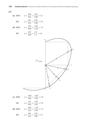
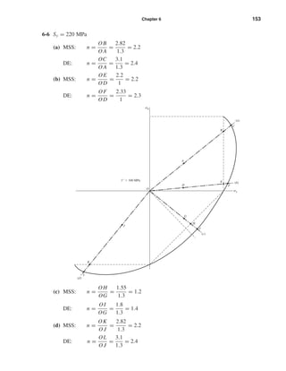
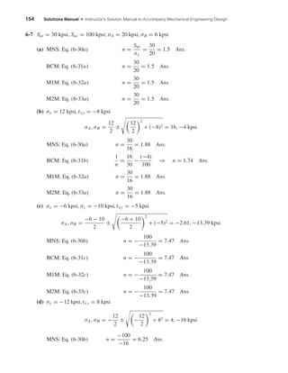
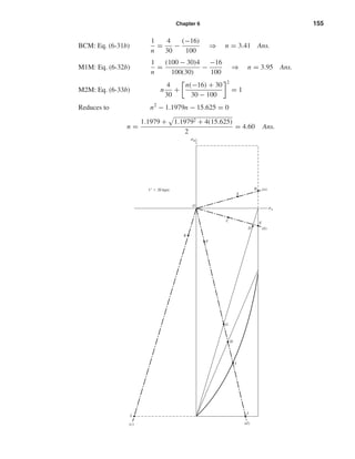
156. 156 Solutions Manual • Instructor’s Solution Manual to Accompany Mechanical Engineering Design
6-8 See Prob. 6-7 for plot.
(a) For all methods: n =
O B
O A
=
1.55
1.03
= 1.5
(b) BCM: n =
O D
OC
=
1.4
0.8
= 1.75
All other methods: n =
OE
OC
=
1.55
0.8
= 1.9
(c) For all methods: n =
OL
OK
=
5.2
0.68
= 7.6
(d) MNS: n =
O J
OF
=
5.12
0.82
= 6.2
BCM: n =
OG
OF
=
2.85
0.82
= 3.5
M1M: n =
O H
OF
=
3.3
0.82
= 4.0
M2M: n =
OI
OF
=
3.82
0.82
= 4.7
6-9 Given: Sy = 42 kpsi, Sut = 66.2 kpsi, εf = 0.90. Sinceεf > 0.05, the material is ductile and
thus we may follow convention by setting Syc = Syt.
Use DE theory for analytical solution. For σ , use Eq. (6-13) or (6-15) for plane stress and
Eq. (6-12) or (6-14) for general 3-D.
(a) σ = [92
− 9(−5) + (−5)2
]1/2
= 12.29 kpsi
n =
42
12.29
= 3.42 Ans.
(b) σ = [122
+ 3(32
)]1/2
= 13.08 kpsi
n =
42
13.08
= 3.21 Ans.
(c) σ = [(−4)2
− (−4)(−9) + (−9)2
+ 3(52
)]1/2
= 11.66 kpsi
n =
42
11.66
= 3.60 Ans.
(d) σ = [112
− (11)(4) + 42
+ 3(12
)]1/2
= 9.798
n =
42
9.798
= 4.29 Ans.
shi20396_ch06.qxd 8/18/03 12:22 PM Page 156

157. Chapter 6 157
For graphical solution, plot load lines on DE envelope as shown.
(a) σA = 9, σB = −5 kpsi
n =
O B
O A
=
3.5
1
= 3.5 Ans.
(b) σA, σB =
12
2
±
12
2
2
+ 32 = 12.7, −0.708 kpsi
n =
O D
OC
=
4.2
1.3
= 3.23
(c) σA, σB =
−4 − 9
2
±
4 − 9
2
2
+ 52 = −0.910, −12.09 kpsi
n =
OF
OE
=
4.5
1.25
= 3.6 Ans.
(d) σA, σB =
11 + 4
2
±
11 − 4
2
2
+ 12 = 11.14, 3.86 kpsi
n =
O H
OG
=
5.0
1.15
= 4.35 Ans.
6-10 This heat-treated steel exhibits Syt = 235 kpsi, Syc = 275 kpsi and εf = 0.06. The steel is
ductile (εf > 0.05) but of unequal yield strengths. The Ductile Coulomb-Mohr hypothesis
(DCM) of Fig. 6-27 applies — confine its use to first and fourth quadrants.
(c)
(a)
(b)
(d)
E
C
G
H
D
B
A
O
F
1 cm ϭ 10 kpsi
␴B
␴A
shi20396_ch06.qxd 8/18/03 12:22 PM Page 157

158. 158 Solutions Manual • Instructor’s Solution Manual to Accompany Mechanical Engineering Design
(a) σx = 90 kpsi, σy = −50 kpsi, σz = 0 І σA = 90 kpsi and σB = −50 kpsi. For the
fourth quadrant, from Eq. (6-13)
n =
1
(σA/Syt) − (σB/Suc)
=
1
(90/235) − (−50/275)
= 1.77 Ans.
(b) σx = 120 kpsi, τxy = −30 kpsi ccw. σA, σB = 127.1, −7.08 kpsi. For the fourth
quadrant
n =
1
(127.1/235) − (−7.08/275)
= 1.76 Ans.
(c) σx = −40 kpsi, σy = −90 kpsi, τxy = 50 kpsi. σA, σB = −9.10, −120.9 kpsi.
Although no solution exists for the third quadrant, use
n = −
Syc
σy
= −
275
−120.9
= 2.27 Ans.
(d) σx = 110 kpsi, σy = 40 kpsi, τxy = 10 kpsi cw. σA, σB = 111.4, 38.6 kpsi. For the
first quadrant
n =
Syt
σA
=
235
111.4
= 2.11 Ans.
Graphical Solution:
(a) n =
O B
O A
=
1.82
1.02
= 1.78
(b) n =
O D
OC
=
2.24
1.28
= 1.75
(c) n =
OF
OE
=
2.75
1.24
= 2.22
(d) n =
O H
OG
=
2.46
1.18
= 2.08
O
(d)
(b)
(a)
(c)
E
F
B
D
G
C
A
H
1 in ϭ 100 kpsi
␴B
␴A
shi20396_ch06.qxd 8/18/03 12:22 PM Page 158

159. Chapter 6 159
6-11 The material is brittle and exhibits unequal tensile and compressive strengths. Decision:
Use the Modified II-Mohr theory as shown in Fig. 6-28 which is limited to first and fourth
quadrants.
Sut = 22 kpsi, Suc = 83 kpsi
Parabolic failure segment:
SA = 22 1 −
SB + 22
22 − 83
2
SB SA SB SA
−22 22.0 −60 13.5
−30 21.6 −70 8.4
−40 20.1 −80 2.3
−50 17.4 −83 0
(a) σx = 9 kpsi, σy = −5 kpsi. σA, σB = 9, −5 kpsi. For the fourth quadrant, use
Eq. (6-33a)
n =
Sut
σA
=
22
9
= 2.44 Ans.
(b) σx = 12 kpsi, τxy = −3 kpsi ccw. σA, σB = 12.7, 0.708 kpsi. For the first quadrant,
n =
Sut
σA
=
22
12.7
= 1.73 Ans.
(c) σx = −4 kpsi, σy = −9 kpsi, τxy = 5 kpsi. σA, σB = −0.910, −12.09 kpsi. For the
third quadrant, no solution exists; however, use Eq. (6-33c)
n =
−83
−12.09
= 6.87 Ans.
(d) σx = 11 kpsi,σy = 4 kpsi,τxy = 1 kpsi.σA, σB = 11.14, 3.86 kpsi. Forthefirstquadrant
n =
SA
σA
=
Syt
σA
=
22
11.14
= 1.97 Ans.
30
30
Sut ϭ 22
Sut ϭ 83
␴B
␴A
–50
–90
shi20396_ch06.qxd 8/18/03 12:22 PM Page 159

160. 160 Solutions Manual • Instructor’s Solution Manual to Accompany Mechanical Engineering Design
6-12 Since εf < 0.05, the material is brittle. Thus, Sut
.
= Suc and we may use M2M which is
basically the same as MNS.
(a) σA, σB = 9, −5 kpsi
n =
35
9
= 3.89 Ans.
(b) σA, σB = 12.7, −0.708 kpsi
n =
35
12.7
= 2.76 Ans.
(c) σA, σB = −0.910, −12.09 kpsi (3rd quadrant)
n =
36
12.09
= 2.98 Ans.
(d) σA, σB = 11.14, 3.86 kpsi
n =
35
11.14
= 3.14 Ans.
Graphical Solution:
(a) n =
O B
O A
=
4
1
= 4.0 Ans.
(b) n =
O D
OC
=
3.45
1.28
= 2.70 Ans.
(c) n =
OF
OE
=
3.7
1.3
= 2.85 Ans. (3rd quadrant)
(d) n =
O H
OG
=
3.6
1.15
= 3.13 Ans.
6-13 Sut = 30 kpsi, Suc = 109 kpsi
Use M2M:
(a) σA, σB = 20, 20 kpsi
Eq. (6-33a): n =
30
20
= 1.5 Ans.
(b) σA, σB = ± (15)2 = 15, −15 kpsi
Eq. (6-33a) n =
30
15
= 2 Ans.
(c) σA, σB = −80, −80 kpsi
For the 3rd quadrant, there is no solution but use Eq. (6-33c).
Eq. (6-33c): n = −
109
−80
= 1.36 Ans.
O
G
C D
A
B
E
F
H
(a)
(c)
(b)
(d)
1 cm ϭ 10 kpsi
␴B
␴A
shi20396_ch06.qxd 8/18/03 12:22 PM Page 160

161. Chapter 6 161
(d) σA, σB = 15, −25 kpsi
Eq. (6-33b):
n(15)
30
+
−25n + 30
30 − 109
2
= 1
n = 1.90 Ans.
(a) n =
O B
O A
=
4.25
2.83
= 1.50
(b) n =
O D
OC
=
4.24
2.12
= 2.00
(c) n =
OF
OE
=
15.5
11.3
= 1.37 (3rd quadrant)
(d) n =
O H
OG
=
5.3
2.9
= 1.83
6-14 Given: AISI 1006 CD steel, F = 0.55 N, P = 8.0 kN, and T = 30 N · m, applying the
DE theory to stress elements A and B with Sy = 280 MPa
A: σx =
32Fl
πd3
+
4P
πd2
=
32(0.55)(103
)(0.1)
π(0.0203)
+
4(8)(103
)
π(0.0202)
= 95.49(106
) Pa = 95.49 MPa
O
(d)
(b)
(a)
(c)
E
F
C
B
A
G
D
H
1 cm ϭ 10 kpsi
␴B
␴A
shi20396_ch06.qxd 8/18/03 12:22 PM Page 161

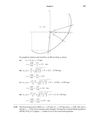
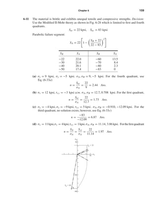
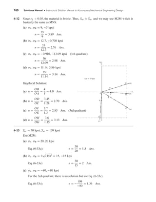
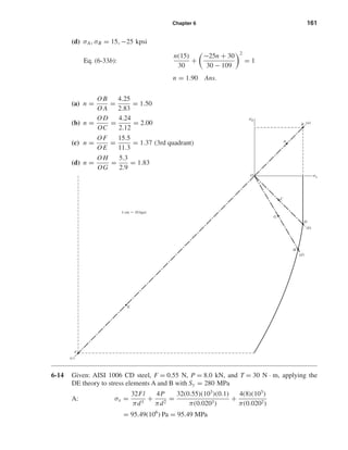
162. 162 Solutions Manual • Instructor’s Solution Manual to Accompany Mechanical Engineering Design
τxy =
16T
πd3
=
16(30)
π(0.0203)
= 19.10(106
) Pa = 19.10 MPa
σ = σ2
x + 3τ2
xy
1/2
= [95.492
+ 3(19.1)2
]1/2
= 101.1 MPa
n =
Sy
σ
=
280
101.1
= 2.77 Ans.
B: σx =
4P
πd3
=
4(8)(103
)
π(0.0202)
= 25.47(106
) Pa = 25.47 MPa
τxy =
16T
πd3
+
4
3
V
A
=
16(30)
π(0.0203)
+
4
3
0.55(103
)
(π/4)(0.0202)
= 21.43(106
) Pa = 21.43 MPa
σ = [25.472
+ 3(21.432
)]1/2
= 45.02 MPa
n =
280
45.02
= 6.22 Ans.
6-15 Design decisions required:
• Material and condition
• Design factor
• Failure model
• Diameter of pin
Using F = 416 lbf from Ex. 6-3
σmax =
32M
πd3
d =
32M
πσmax
1/3
Decision 1: Select the same material and condition of Ex. 6-3 (AISI 1035 steel, Sy =
81 000).
Decision 2: Since we prefer the pin to yield, set nd a little larger than 1. Further explana-
tion will follow.
Decision 3: Use the Distortion Energy static failure theory.
Decision 4: Initially set nd = 1
σmax =
Sy
nd
=
Sy
1
= 81 000 psi
d =
32(416)(15)
π(81 000)
1/3
= 0.922 in
shi20396_ch06.qxd 8/18/03 12:22 PM Page 162

163. Chapter 6 163
Choose preferred size of d = 1.000 in
F =
π(1)3
(81 000)
32(15)
= 530 lbf
n =
530
416
= 1.274
Set design factor to nd = 1.274
Adequacy Assessment:
σmax =
Sy
nd
=
81 000
1.274
= 63 580 psi
d =
32(416)(15)
π(63 580)
1/3
= 1.000 in (OK )
F =
π(1)3
(81 000)
32(15)
= 530 lbf
n =
530
416
= 1.274 (OK)
6-16 For a thin walled cylinder made of AISI 1018 steel, Sy = 54 kpsi, Sut = 64 kpsi.
The state of stress is
σt =
pd
4t
=
p(8)
4(0.05)
= 40p, σl =
pd
8t
= 20p, σr = −p
These three are all principal stresses. Therefore,
σ =
1
√
2
[(σ1 − σ2)2
+ (σ2 − σ3)2
+ (σ3 − σ1)2
]1/2
=
1
√
2
[(40p − 20p)2
+ (20p + p)2
+ (−p − 40p)2
]
= 35.51p = 54 ⇒ p = 1.52 kpsi (for yield) Ans.
For rupture, 35.51p
.
= 64 ⇒ p
.
= 1.80 kpsi Ans.
6-17 For hot-forgedAISI steelw = 0.282 lbf/in3
, Sy = 30 kpsi and ν = 0.292. Then ρ = w/g =
0.282/386 lbf · s2
/in;ri = 3 in;ro = 5 in;r2
i = 9;r2
o = 25; 3 + ν = 3.292; 1 + 3ν =1.876.
Eq. (4-56) for r = ri becomes
σt = ρω2 3 + ν
8
2r2
o + r2
i 1 −
1 + 3ν
3 + ν
Rearranging and substituting the above values:
Sy
ω2
=
0.282
386
3.292
8
50 + 9 1 −
1.876
3.292
= 0.016 19
shi20396_ch06.qxd 8/18/03 12:22 PM Page 163

164. 164 Solutions Manual • Instructor’s Solution Manual to Accompany Mechanical Engineering Design
Setting the tangential stress equal to the yield stress,
ω =
30 000
0.016 19
1/2
= 1361 rad/s
or n = 60ω/2π = 60(1361)/(2π)
= 13 000 rev/min
Now check the stresses at r = (rori )1/2
, or r = [5(3)]1/2
= 3.873 in
σr = ρω2 3 + ν
8
(ro − ri )2
=
0.282ω2
386
3.292
8
(5 − 3)2
= 0.001 203ω2
Applying Eq. (4-56) for σt
σt = ω2 0.282
386
3.292
8
9 + 25 +
9(25)
15
−
1.876(15)
3.292
= 0.012 16ω2
Using the Distortion-Energy theory
σ = σ2
t − σr σt + σ2
r
1/2
= 0.011 61ω2
Solving ω =
30 000
0.011 61
1/2
= 1607 rad/s
So the inner radius governs and n = 13 000 rev/min Ans.
6-18 For a thin-walled pressure vessel,
di = 3.5 − 2(0.065) = 3.37 in
σt =
p(di + t)
2t
σt =
500(3.37 + 0.065)
2(0.065)
= 13 212 psi
σl =
pdi
4t
=
500(3.37)
4(0.065)
= 6481 psi
σr = −pi = −500 psi
shi20396_ch06.qxd 8/18/03 12:22 PM Page 164

165. Chapter 6 165
These are all principal stresses, thus,
σ =
1
√
2
{(13 212 − 6481)2
+ [6481 − (−500)]2
+ (−500 − 13 212)2
}1/2
σ = 11 876 psi
n =
Sy
σ
=
46 000
σ
=
46 000
11 876
= 3.87 Ans.
6-19 Table A-20 gives Sy as 320 MPa. The maximum significant stress condition occurs at ri
where σ1 = σr = 0, σ2 = 0, and σ3 = σt. From Eq. (4-50) for r = ri
σt = −
2r2
o po
r2
o − r2
i
= −
2(1502
) po
1502 − 1002
= −3.6po
σ = 3.6po = Sy = 320
po =
320
3.6
= 88.9 MPa Ans.
6-20 Sut = 30 kpsi, w = 0.260 lbf/in3
, ν = 0.211, 3 + ν = 3.211, 1 + 3ν = 1.633. At the inner
radius, from Prob. 6-17
σt
ω2
= ρ
3 + ν
8
2r2
o + r2
i −
1 + 3ν
3 + ν
r2
i
Here r2
o = 25, r2
i = 9, and so
σt
ω2
=
0.260
386
3.211
8
50 + 9 −
1.633(9)
3.211
= 0.0147
Since σr is of the same sign, we use M2M failure criteria in the first quadrant. From Table
A-24, Sut = 31 kpsi, thus,
ω =
31 000
0.0147
1/2
= 1452 rad/s
rpm = 60ω/(2π) = 60(1452)/(2π)
= 13 866 rev/min
Using the grade number of 30 for Sut = 30 000 kpsi gives a bursting speed of 13640 rev/min.
6-21 TC = (360 − 27)(3) = 1000 lbf · in, TB = (300 − 50)(4) = 1000 lbf · in
B
A D
C
223 lbf
8" 8" 6"
350 lbf
127 lbf
xy plane
y
shi20396_ch06.qxd 8/18/03 12:22 PM Page 165

166. 166 Solutions Manual • Instructor’s Solution Manual to Accompany Mechanical Engineering Design
In xy plane, MB = 223(8) = 1784 lbf · in and MC = 127(6) = 762 lbf · in.
In the xz plane, MB = 848 lbf · in and MC = 1686 lbf · in. The resultants are
MB = [(1784)2
+ (848)2
]1/2
= 1975 lbf · in
MC = [(1686)2
+ (762)2
]1/2
= 1850 lbf · in
So point B governs and the stresses are
τxy =
16T
πd3
=
16(1000)
πd3
=
5093
d3
psi
σx =
32MB
πd3
=
32(1975)
πd3
=
20 120
d3
psi
Then
σA, σB =
σx
2
±
σx
2
2
+ τ2
xy
1/2
σA, σB =
1
d3



20.12
2
±
20.12
2
2
+ (5.09)2
1/2



=
(10.06 ± 11.27)
d3
kpsi · in3
Then
σA =
10.06 + 11.27
d3
=
21.33
d3
kpsi
and
σB =
10.06 − 11.27
d3
= −
1.21
d3
kpsi
For this state of stress, use the Brittle-Coulomb-Mohr theory for illustration. Here we use
Sut(min) = 25 kpsi, Suc(min) = 97 kpsi, and Eq. (6-31b) to arrive at
21.33
25d3
−
−1.21
97d3
=
1
2.8
Solving gives d = 1.34 in. So use d = 1 3/8 in Ans.
Note that this has been solved as a statics problem. Fatigue will be considered in the next
chapter.
6-22 As in Prob. 6-21, we will assume this to be statics problem. Since the proportions are un-
changed, the bearing reactions will be the same as in Prob. 6-21. Thus
xy plane: MB = 223(4) = 892 lbf · in
xz plane: MB = 106(4) = 424 lbf · in
B
A D
C
xz plane
106 lbf
8" 8" 6"
281 lbf
387 lbf
shi20396_ch06.qxd 8/27/03 4:38 PM Page 166

167. Chapter 6 167
So
Mmax = [(892)2
+ (424)2
]1/2
= 988 lbf · in
σx =
32MB
πd3
=
32(988)
πd3
=
10 060
d3
psi
Since the torsional stress is unchanged,
τxz = 5.09/d3
kpsi
σA, σB =
1
d3



10.06
2
±
10.06
2
2
+ (5.09)2
1/2



σA = 12.19/d3
and σB = −2.13/d3
Using the Brittle-Coulomb-Mohr, as was used in Prob. 6-21, gives
12.19
25d3
−
−2.13
97d3
=
1
2.8
Solving gives d = 1 1/8 in. Now compare to Modified II-Mohr theory Ans.
6-23 (FA)t = 300 cos 20 = 281.9 lbf, (FA)r = 300 sin 20 = 102.6 lbf
T = 281.9(12) = 3383 lbf · in, (FC)t =
3383
5
= 676.6 lbf
(FC)r = 676.6 tan 20 = 246.3 lbf
MA = 20 193.72 + 233.52 = 6068 lbf · in
MB = 10 246.32 + 676.62 = 7200 lbf · in (maximum)
σx =
32(7200)
πd3
=
73 340
d3
τxy =
16(3383)
πd3
=
17 230
d3
σ = σ2
x + 3τ2
xy
1/2
=
Sy
n
73 340
d3
2
+ 3
17 230
d3
2 1/2
=
79 180
d3
=
60 000
3.5
d = 1.665 in so use a standard diameter size of 1.75 in Ans.
xy plane
x
y
A B C
ROy = 193.7 lbf
RBy = 158.1 lbf
281.9 lbf
20" 16" 10"
246.3 lbf
O
xz plane
x
z
A B C
ROz = 233.5 lbf
RBz = 807.5 lbf
O
102.6 lbf
20" 16" 10"
676.6 lbf
shi20396_ch06.qxd 8/18/03 12:22 PM Page 167

168. 168 Solutions Manual • Instructor’s Solution Manual to Accompany Mechanical Engineering Design
6-24 From Prob. 6-23,
τmax =
σx
2
2
+ τ2
xy
1/2
=
Sy
2n
73 340
2d3
2
+
17 230
d3
2 1/2
=
40 516
d3
=
60 000
2(3.5)
d = 1.678 in so use 1.75 in Ans.
6-25 T = (270 − 50)(0.150) = 33 N · m, Sy = 370 MPa
(T1 − 0.15T1)(0.125) = 33 ⇒ T1 = 310.6 N, T2 = 0.15(310.6) = 46.6 N
(T1 + T2) cos 45 = 252.6 N
MA = 0.3 163.42 + 1072 = 58.59 N · m (maximum)
MB = 0.15 89.22 + 174.42 = 29.38 N · m
σx =
32(58.59)
πd3
=
596.8
d3
τxy =
16(33)
πd3
=
168.1
d3
σ = σ2
x + 3τ2
xy
1/2
=
596.8
d3
2
+ 3
168.1
d3
2 1/2
=
664.0
d3
=
370(106
)
3.0
d = 17.5(10−3
) m = 17.5 mm, so use 18 mm Ans.
6-26 From Prob. 6-25,
τmax =
σx
2
2
+ τ2
xy
1/2
=
Sy
2n
596.8
2d3
2
+
168.1
d3
2 1/2
=
342.5
d3
=
370(106
)
2(3.0)
d = 17.7(10−3
) m = 17.7 mm, so use 18 mm Ans.
xz plane
z
107.0 N
174.4 N
252.6 N
320 N
300 400 150
y
163.4 N 89.2 N252.6 N
300 400 150
xy plane
A
B C
O
shi20396_ch06.qxd 8/18/03 12:22 PM Page 168

169. Chapter 6 169
6-27 For the loading scheme shown in Figure (c),
Mmax =
F
2
a
2
+
b
4
=
4.4
2
(6 + 4.5)
= 23.1 N · m
For a stress element at A:
σx =
32M
πd3
=
32(23.1)(103
)
π(12)3
= 136.2 MPa
The shear at C is
τxy =
4(F/2)
3πd2/4
=
4(4.4/2)(103
)
3π(12)2/4
= 25.94 MPa
τmax =
136.2
2
2 1/2
= 68.1 MPa
Since Sy = 220 MPa, Ssy = 220/2 = 110 MPa, and
n =
Ssy
τmax
=
110
68.1
= 1.62 Ans.
For the loading scheme depicted in Figure (d)
Mmax =
F
2
a + b
2
−
F
2
1
2
b
2
2
=
F
2
a
2
+
b
4
This result is the same as that obtained for Figure (c). At point B, we also have a surface
compression of
σy =
−F
A
=
−F
bd
−
−4.4(103
)
18(12)
= −20.4 MPa
With σx = −136.2 MPa. From a Mohrs circle diagram, τmax = 136.2/2 = 68.1 MPa.
n =
110
68.1
= 1.62 MPa Ans.
6-28 Based on Figure (c) and using Eq. (6-15)
σ = σ2
x
1/2
= (136.22
)1/2
= 136.2 MPa
n =
Sy
σ
=
220
136.2
= 1.62 Ans.
x
y
A
B
V
M
C
shi20396_ch06.qxd 8/18/03 12:22 PM Page 169

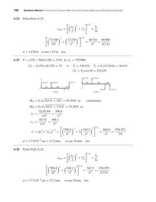
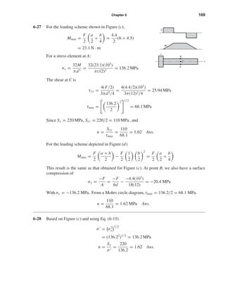
170. 170 Solutions Manual • Instructor’s Solution Manual to Accompany Mechanical Engineering Design
Based on Figure (d) and using Eq. (6-15) and the solution of Prob. 6-27,
σ = σ2
x − σxσy + σ2
y
1/2
= [(−136.2)2
− (−136.2)(−20.4) + (−20.4)2
]1/2
= 127.2 MPa
n =
Sy
σ
=
220
127.2
= 1.73 Ans.
6-29
When the ring is set, the hoop tension in the ring is
equal to the screw tension.
σt =
r2
i pi
r2
o − r2
i
1 +
r2
o
r2
We have the hoop tension at any radius. The differential hoop tension dF is
dF = wσt dr
F =
ro
ri
wσt dr =
wr2
i pi
r2
o − r2
i
ro
ri
1 +
r2
o
r2
dr = wri pi (1)
The screw equation is
Fi =
T
0.2d
(2)
From Eqs. (1) and (2)
pi =
F
wri
=
T
0.2dwri
dFx = f piri dθ
Fx =
2π
o
f pi wri dθ =
f Tw
0.2dwri
ri
2π
o
dθ
=
2π f T
0.2d
Ans.
6-30
(a) From Prob. 6-29, T = 0.2Fi d
Fi =
T
0.2d
=
190
0.2(0.25)
= 3800 lbf Ans.
(b) From Prob. 6-29, F = wri pi
pi =
F
wri
=
Fi
wri
=
3800
0.5(0.5)
= 15 200 psi Ans.
dFx
piri d␪
dF
r
w
shi20396_ch06.qxd 8/18/03 12:22 PM Page 170

171. Chapter 6 171
(c) σt =
r2
i pi
r2
o − r2
i
1 +
r2
o
r r=ri
=
pi r2
i + r2
o
r2
o − r2
i
=
15 200(0.52
+ 12
)
12 − 0.52
= 25 333 psi Ans.
σr = −pi = −15 200 psi
(d) τmax =
σ1 − σ3
2
=
σt − σr
2
=
25 333 − (−15 200)
2
= 20 267 psi Ans.
σ = σ2
A + σ2
B − σAσB
1/2
= [25 3332
+ (−15 200)2
− 25 333(−15 200)]1/2
= 35 466 psi Ans.
(e) Maximum Shear hypothesis
n =
Ssy
τmax
=
0.5Sy
τmax
=
0.5(63)
20.267
= 1.55 Ans.
Distortion Energy theory
n =
Sy
σ
=
63
35 466
= 1.78 Ans.
6-31
The moment about the center caused by force F
is Fre where re is the effective radius. This is
balanced by the moment about the center
caused by the tangential (hoop) stress.
Fre =
ro
ri
rσtw dr
=
wpir2
i
r2
o − r2
i
ro
ri
r +
r2
o
r
dr
re =
wpir2
i
F r2
o − r2
i
r2
o − r2
i
2
+ r2
o ln
ro
ri
From Prob. 6-29, F = wri pi . Therefore,
re =
ri
r2
o − r2
i
r2
o − r2
i
2
+ r2
o ln
ro
ri
For the conditions of Prob. 6-29, ri = 0.5 and ro = 1 in
re =
0.5
12 − 0.52
12
− 0.52
2
+ 12
ln
1
0.5
= 0.712 in
R
␴t
1
2
"
1"R
re
r
shi20396_ch06.qxd 8/18/03 12:22 PM Page 171

172. 172 Solutions Manual • Instructor’s Solution Manual to Accompany Mechanical Engineering Design
6-32 δnom = 0.0005 in
(a) From Eq. (4-60)
p =
30(106
)(0.0005)
1
(1.52
− 12
)(12
− 0.52
)
2(12)(1.52 − 0.52)
= 3516 psi Ans.
Inner member:
Eq. (4-57) (σt)i = −p
R2
+ r2
i
R2 − r2
i
= −3516
12
+ 0.52
12 − 0.52
= −5860 psi
(σr )i = −p = −3516 psi
Eq. (6-13) σi = σ2
A − σAσB + σ2
B
1/2
= [(−5860)2
− (−5860)(−3516) + (−3516)2
]1/2
= 5110 psi Ans.
Outer member:
Eq. (4-58) (σt)o = 3516
1.52
+ 12
1.52 − 12
= 9142 psi
(σr )o = −p = −3516 psi
Eq. (6-13) σo = [91422
− 9142(−3516) + (−3516)2
]1/2
= 11 320 psi Ans.
(b) For a solid inner tube,
p =
30(106
)(0.0005)
1
(1.52
− 12
)(12
)
2(12)(1.52)
= 4167 psi Ans.
(σt)i = −p = −4167 psi, (σr )i = −4167 psi
σi = [(−4167)2
− (−4167)(−4167) + (−4167)2
]1/2
= 4167 psi Ans.
(σt)o = 4167
1.52
+ 12
1.52 − 12
= 10 830 psi, (σr )o = −4167 psi
σo = [10 8302
− 10 830(−4167) + (−4167)2
]1/2
= 13 410 psi Ans.
6-33 Using Eq. (4-60) with diametral values,
p =
207(103
)(0.02)
50
(752
− 502
)(502
− 252
)
2(502)(752 − 252)
= 19.41 MPa Ans.
Eq. (4-57) (σt)i = −19.41
502
+ 252
502 − 252
= −32.35 MPa
(σr )i = −19.41 MPa
Eq. (6-13) σi = [(−32.35)2
− (−32.35)(−19.41) + (−19.41)2
]1/2
= 28.20 MPa Ans.
shi20396_ch06.qxd 8/18/03 12:22 PM Page 172

173. Chapter 6 173
Eq. (4-58) (σt)o = 19.41
752
+ 502
752 − 502
= 50.47 MPa,
(σr )o = −19.41 MPa
σo = [50.472
− 50.47(−19.41) + (−19.41)2
]1/2
= 62.48 MPa Ans.
6-34
δ =
1.9998
2
−
1.999
2
= 0.0004 in
Eq. (4-59)
0.0004 =
p(1)
14.5(106)
22
+ 12
22 − 12
+ 0.211 +
p(1)
30(106)
12
+ 0
12 − 0
− 0.292
p = 2613 psi
Applying Eq. (4-58) at R,
(σt)o = 2613
22
+ 12
22 − 12
= 4355 psi
(σr )o = −2613 psi, Sut = 20 kpsi, Suc = 83 kpsi
Eq. (6-33b)
n(4355)
20 000
+
−2613n + 20 000
20 000 − 83 000
2
= 1
n = 4.52 Ans.
6-35 E = 30(106
) psi, ν = 0.292, I = (π/64)(24
− 1.54
) = 0.5369 in4
Eq. (4-60) can be written in terms of diameters,
p =
Eδd
D
d2
o − D2
D2
− d2
i
2D2 d2
o − d2
i
=
30(106
)
1.75
(0.002 46)
(22
− 1.752
)(1.752
− 1.52
)
2(1.752)(22 − 1.52)
= 2997 psi = 2.997 kpsi
Outer member:
Outer radius: (σt)o =
1.752
(2.997)
22 − 1.752
(2) = 19.58 kpsi, (σr )o = 0
Inner radius: (σt)i =
1.752
(2.997)
22 − 1.752
1 +
22
1.752
= 22.58 kpsi, (σr )i = −2.997 kpsi
Bending:
ro: (σx)o =
6.000(2/2)
0.5369
= 11.18 kpsi
ri : (σx)i =
6.000(1.75/2)
0.5369
= 9.78 kpsi
shi20396_ch06.qxd 8/18/03 12:22 PM Page 173

174. 174 Solutions Manual • Instructor’s Solution Manual to Accompany Mechanical Engineering Design
Torsion: J = 2I = 1.0738 in4
ro: (τxy)o =
8.000(2/2)
1.0738
= 7.45 kpsi
ri : (τxy)i =
8.000(1.75/2)
1.0738
= 6.52 kpsi
Outer radius is plane stress
σx = 11.18 kpsi, σy = 19.58 kpsi, τxy = 7.45 kpsi
Eq. (6-15) σ = [11.182
− (11.18)(19.58) + 19.582
+ 3(7.452
)]1/2
=
Sy
no
=
60
no
21.35 =
60
no
⇒ no = 2.81 Ans.
Inner radius, 3D state of stress
From Eq. (6-14) with τyz = τzx = 0
σ =
1
√
2
[(9.78 − 22.58)2
+ (22.58 + 2.997)2
+ (−2.997 − 9.78)2
+ 6(6.52)2
]1/2
=
60
ni
24.86 =
60
ni
⇒ ni = 2.41 Ans.
6-36 From Prob. 6-35: p = 2.997 kpsi, I = 0.5369 in4
, J = 1.0738 in4
Inner member:
Outer radius: (σt)o = −2.997
(0.8752
+ 0.752
)
(0.8752 − 0.752)
= −19.60 kpsi
(σr )o = −2.997 kpsi
Inner radius: (σt)i = −
2(2.997)(0.8752
)
0.8752 − 0.752
= −22.59 kpsi
(σr )i = 0
Bending:
ro: (σx)o =
6(0.875)
0.5369
= 9.78 kpsi
ri : (σx)i =
6(0.75)
0.5369
= 8.38 kpsi
yx
–2.997 kpsi
9.78 kpsi
22.58 kpsi
6.52 kpsi
z
shi20396_ch06.qxd 8/18/03 12:22 PM Page 174

175. Chapter 6 175
Torsion:
ro: (τxy)o =
8(0.875)
1.0738
= 6.52 kpsi
ri : (τxy)i =
8(0.75)
1.0738
= 5.59 kpsi
The inner radius is in plane stress: σx = 8.38 kpsi, σy = −22.59 kpsi, τxy = 5.59 kpsi
σi = [8.382
− (8.38)(−22.59) + (−22.59)2
+ 3(5.592
)]1/2
= 29.4 kpsi
ni =
Sy
σi
=
60
29.4
= 2.04 Ans.
Outer radius experiences a radial stress, σr
σo =
1
√
2
(−19.60 + 2.997)2
+ (−2.997 − 9.78)2
+ (9.78 + 19.60)2
+ 6(6.52)2 1/2
= 27.9 kpsi
no =
60
27.9
= 2.15 Ans.
6-37
σp =
1
2
2
KI
√
2πr
cos
θ
2
±
KI
√
2πr
sin
θ
2
cos
θ
2
sin
3θ
2
2
+
KI
√
2πr
sin
θ
2
cos
θ
2
cos
3θ
2
2 1/2
=
KI
√
2πr
cos
θ
2
± sin2 θ
2
cos2 θ
2
sin2 3θ
2
+ sin2 θ
2
cos2 θ
2
cos2 3θ
2
1/2
=
KI
√
2πr
cos
θ
2
± cos
θ
2
sin
θ
2
=
KI
√
2πr
cos
θ
2
1 ± sin
θ
2
Plane stress: The third principal stress is zero and
σ1 =
KI
√
2πr
cos
θ
2
1 + sin
θ
2
, σ2 =
KI
√
2πr
cos
θ
2
1 − sin
θ
2
, σ3 = 0 Ans.
Plane strain: σ1 and σ2 equations still valid however,
σ3 = ν(σx + σy) = 2ν
KI
√
2πr
cos
θ
2
Ans.
6-38 For θ = 0 and plane strain, the principal stress equations of Prob. 6-37 give
σ1 = σ2 =
KI
√
2πr
, σ3 = 2ν
KI
√
2πr
= 2νσ1
shi20396_ch06.qxd 8/18/03 12:22 PM Page 175

176. 176 Solutions Manual • Instructor’s Solution Manual to Accompany Mechanical Engineering Design
(a) DE:
1
√
2
[(σ1 − σ1)2
+ (σ1 − 2νσ1)2
+ (2νσ1 − σ1)2
]1/2
= Sy
σ1 − 2νσ1 = Sy
For ν =
1
3
, 1 − 2
1
3
σ1 = Sy ⇒ σ1 = 3Sy Ans.
(b) MSS: σ1 − σ3 = Sy ⇒ σ1 − 2νσ1 = Sy
ν =
1
3
⇒ σ1 = 3Sy Ans.
σ3 =
2
3
σ1
Radius of largest circle
R =
1
2
σ1 −
2
3
σ1 =
σ1
6
6-39 (a) Ignoring stress concentration
F = Sy A = 160(4)(0.5) = 320 kips Ans.
(b) From Fig. 6-36: h/b = 1, a/b = 0.625/4 = 0.1563, β = 1.3
Eq. (6-51) 70 = 1.3
F
4(0.5)
π(0.625)
F = 76.9 kips Ans.
6-40 Given: a = 12.5 mm, KIc = 80 MPa ·
√
m, Sy = 1200 MPa, Sut = 1350 MPa
ro =
350
2
= 175 mm, ri =
350 − 50
2
= 150 mm
a/(ro − ri ) =
12.5
175 − 150
= 0.5
ri /ro =
150
175
= 0.857
Fig. 6-40: β
.
= 2.5
Eq. (6-51): KIc = βσ
√
πa
80 = 2.5σ π(0.0125)
σ = 161.5 MPa
␴1, ␴2
␴
␴1
␶
2
3
shi20396_ch06.qxd 8/18/03 12:22 PM Page 176

177. Chapter 6 177
Eq. (4-51) at r = ro:
σ =
r2
i pi
r2
o − r2
i
(2)
161.5 =
1502
pi (2)
1752 − 1502
pi = 29.2 MPa Ans.
6-41
(a) First convert the data to radial dimensions to agree with the formulations of Fig. 4-25.
Thus
ro = 0.5625 ± 0.001in
ri = 0.1875 ± 0.001in
Ro = 0.375 ± 0.0002in
Ri = 0.376 ± 0.0002in
The stochastic nature of the dimensions affects the δ = |Ri | − |Ro| relation in
Eq. (4-60) but not the others. Set R = (1/2)(Ri + Ro) = 0.3755. From Eq. (4-60)
p =
Eδ
R
r2
o − R2
R2
− r2
i
2R2 r2
o − r2
i
Substituting and solving with E = 30 Mpsi gives
p = 18.70(106
) δ
Since δ = Ri − Ro
¯δ = ¯Ri − ¯Ro = 0.376 − 0.375 = 0.001 in
and
ˆσδ =
0.0002
4
2
+
0.0002
4
2 1/2
= 0.000 070 7 in
Then
Cδ =
ˆσδ
¯δ
=
0.000 070 7
0.001
= 0.0707
The tangential inner-cylinder stress at the shrink-fit surface is given by
σit = −p
¯R2
+ ¯r2
i
¯R2 − ¯r2
i
= −18.70(106
) δ
0.37552
+ 0.18752
0.37552 − 0.18752
= −31.1(106
) δ
¯σit = −31.1(106
) ¯δ = −31.1(106
)(0.001)
= −31.1(103
) psi
shi20396_ch06.qxd 8/18/03 12:22 PM Page 177

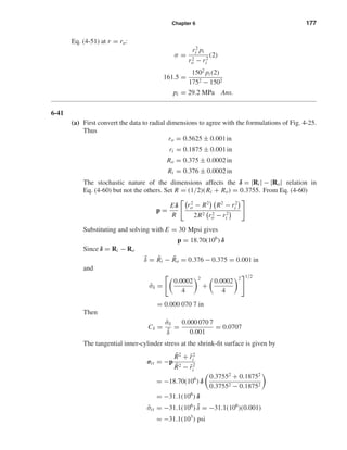
178. 178 Solutions Manual • Instructor’s Solution Manual to Accompany Mechanical Engineering Design
Also
ˆσσit
= |Cδ ¯σit| = 0.0707(−31.1)103
= 2899 psi
σit = N(−31 100, 2899) psi Ans.
(b) The tangential stress for the outer cylinder at the shrink-fit surface is given by
σot = p
¯r2
o + ¯R2
¯r2
o − ¯R2
= 18.70(106
) δ
0.56252
+ 0.37552
0.56252 − 0.37552
= 48.76(106
) δ psi
¯σot = 48.76(106
)(0.001) = 48.76(103
) psi
ˆσσot
= Cδ ¯σot = 0.0707(48.76)(103
) = 34.45 psi
І σot = N(48 760, 3445) psi Ans.
6-42 From Prob. 6-41, at the fit surface σot = N(48.8, 3.45) kpsi. The radial stress is the fit
pressure which was found to be
p = 18.70(106
) δ
¯p = 18.70(106
)(0.001) = 18.7(103
) psi
ˆσp = Cδ ¯p = 0.0707(18.70)(103
)
= 1322 psi
and so
p = N(18.7, 1.32) kpsi
and
σor = −N(18.7, 1.32) kpsi
These represent the principal stresses. The von Mises stress is next assessed.
¯σA = 48.8 kpsi, ¯σB = −18.7 kpsi
k = ¯σB/¯σA = −18.7/48.8 = −0.383
¯σ = ¯σA(1 − k + k2
)1/2
= 48.8[1 − (−0.383) + (−0.383)2
]1/2
= 60.4 kpsi
ˆσσ = Cp ¯σ = 0.0707(60.4) = 4.27 kpsi
shi20396_ch06.qxd 8/18/03 12:22 PM Page 178

179. Chapter 6 179
Using the interference equation
z = −
¯S − ¯σ
ˆσ2
S + ˆσ2
σ
1/2
= −
95.5 − 60.4
[(6.59)2 + (4.27)2]1/2
= −4.5
pf = α = 0.000 003 40,
or about 3 chances in a million. Ans.
6-43
σt =
pd
2t
=
6000N(1, 0.083 33)(0.75)
2(0.125)
= 18N(1, 0.083 33) kpsi
σl =
pd
4t
=
6000N(1, 0.083 33)(0.75)
4(0.125)
= 9N(1, 0.083 33) kpsi
σr = −p = −6000N(1, 0.083 33) kpsi
These three stresses are principal stresses whose variability is due to the loading. From
Eq. (6-12), we find the von Mises stress to be
σ =
(18 − 9)2
+ [9 − (−6)]2
+ (−6 − 18)2
2
1/2
= 21.0 kpsi
ˆσσ = Cp ¯σ = 0.083 33(21.0) = 1.75 kpsi
z = −
¯S − ¯σ
ˆσ2
S + ˆσ2
σ
1/2
=
50 − 21.0
(4.12 + 1.752)1/2
= −6.5
The reliability is very high
R = 1 − (6.5) = 1 − 4.02(10−11
)
.
= 1 Ans.
shi20396_ch06.qxd 8/18/03 12:22 PM Page 179

180. Chapter 7
7-1 HB = 490
Eq. (3-17): Sut = 0.495(490) = 242.6 kpsi > 212 kpsi
Eq. (7-8): Se = 107 kpsi
Table 7-4: a = 1.34, b = −0.085
Eq. (7-18): ka = 1.34(242.6)−0.085
= 0.840
Eq. (7-19): kb =
3/16
0.3
−0.107
= 1.05
Eq. (7-17): Se = kakbSe = 0.840(1.05)(107) = 94.4 kpsi Ans.
7-2
(a) Sut = 68 kpsi, Se = 0.495(68) = 33.7 kpsi Ans.
(b) Sut = 112 kpsi, Se = 0.495(112) = 55.4 kpsi Ans.
(c) 2024T3 has no endurance limit Ans.
(d) Eq. (3-17): Se = 107 kpsi Ans.
7-3
σF = σ0εm = 115(0.90)0.22
= 112.4 kpsi
Eq. (7-8): Se = 0.504(66.2) = 33.4 kpsi
Eq. (7-11): b = −
log(112.4/33.4)
log(2 · 106)
= −0.083 64
Eq. (7-9): f =
112.4
66.2
(2 · 103
)−0.083 64
= 0.8991
Eq. (7-13): a =
[0.8991(66.2)]2
33.4
= 106.1 kpsi
Eq. (7-12): Sf = aNb
= 106.1(12 500)−0.083 64
= 48.2 kpsi Ans.
Eq. (7-15): N =
σa
a
1/b
=
36
106.1
−1/0.083 64
= 409 530 cycles Ans.
7-4 From Sf = aNb
log Sf = log a + b log N
Substituting (1, Sut)
log Sut = log a + b log (1)
From which a = Sut
shi20396_ch07.qxd 8/18/03 12:35 PM Page 180

181. Chapter 7 181
Substituting (103
, f Sut) and a = Sut
log f Sut = log Sut + b log 103
From which
b =
1
3
log f
∴ Sf = Sut N(log f )/3
1 ≤ N ≤ 103
For 500 cycles as in Prob. 7-3
500Sf ≥ 66.2(500)(log 0.8991)/3
= 60.2 kpsi Ans.
7-5 Read from graph: (103
, 90) and (106
, 50). From S = aNb
log S1 = log a + b log N1
log S2 = log a + b log N2
From which
log a =
log S1 log N2 − log S2 log N1
log N2/N1
=
log 90 log 106
− log 50 log 103
log 106/103
= 2.2095
a = 10log a
= 102.2095
= 162.0
b =
log 50/90
3
= −0.085 09
(Sf )ax = 162−0.085 09
103
≤ N ≤ 106
in kpsi Ans.
Check:
103
(Sf )ax = 162(103
)−0.085 09
= 90 kpsi
106
(Sf )ax = 162(106
)−0.085 09
= 50 kpsi
The end points agree.
7-6
Eq. (7-8): Se = 0.504(710) = 357.8 MPa
Table 7-4: a = 4.51, b = −0.265
Eq. (7-18): ka = 4.51(710)−0.265
= 0.792
Eq. (7-19): kb =
d
7.62
−0.107
=
32
7.62
−0.107
= 0.858
Eq. (7-17): Se = kakbSe = 0.792(0.858)(357.8) = 243 MPa Ans.
shi20396_ch07.qxd 8/18/03 12:35 PM Page 181

182. 182 Solutions Manual • Instructor’s Solution Manual to Accompany Mechanical Engineering Design
7-7 For AISI 4340 as forged steel,
Eq. (7-8): Se = 107 kpsi
Table 7-4: a = 39.9, b = −0.995
Eq. (7-18): ka = 39.9(260)−0.995
= 0.158
Eq. (7-19): kb =
0.75
0.30
−0.107
= 0.907
Each of the other Marin factors is unity.
Se = 0.158(0.907)(107) = 15.3 kpsi
For AISI 1040:
Se = 0.504(113) = 57.0 kpsi
ka = 39.9(113)−0.995
= 0.362
kb = 0.907 (same as 4340)
Each of the other Marin factors is unity.
Se = 0.362(0.907)(57.2) = 18.7 kpsi
Not only is AISI 1040 steel a contender, it has a superior endurance strength. Can you see
why?
7-8
(a) For an AISI 1018 CD-machined steel, the strengths are
Eq. (3-17): Sut = 440 MPa ⇒ HB =
440
3.41
= 129
Sy = 370 MPa
Ssu = 0.67(440) = 295 MPa
Fig. A-15-15:
r
d
=
2.5
20
= 0.125,
D
d
=
25
20
= 1.25, Kts = 1.4
Fig. 7-21: qs = 0.94
Eq. (7-31): Kf s = 1 + 0.94(1.4 − 1) = 1.376
For a purely reversing torque of 200 N · m
τmax =
Kf s16T
πd3
=
1.376(16)(200 × 103
N · mm)
π(20 mm)3
τmax = 175.2 MPa = τa
Se = 0.504(440) = 222 MPa
The Marin factors are
ka = 4.51(440)−0.265
= 0.899
kb =
20
7.62
−0.107
= 0.902
kc = 0.59, kd = 1, ke = 1
Eq. (7-17): Se = 0.899(0.902)(0.59)(222) = 106.2 MPa
2.5 mm
20 mm 25 mm
shi20396_ch07.qxd 8/18/03 12:35 PM Page 182

183. Chapter 7 183
Eq. (7-13): a =
[0.9(295)]2
106.2
= 664
Eq. (7-14): b = −
1
3
log
0.9(295)
106.2
= −0.132 65
Eq. (7-15): N =
175.2
664
1/−0.132 65
N = 23 000 cycles Ans.
(b) For an operating temperature of 450°C, the temperature modification factor, from
Table 7-6, is
kd = 0.843
Thus Se = 0.899(0.902)(0.59)(0.843)(222) = 89.5 MPa
a =
[0.9(295)]2
89.5
= 788
b = −
1
3
log
0.9(295)
89.5
= −0.157 41
N =
175.2
788
1/−0.157 41
N = 14 100 cycles Ans.
7-9
f = 0.9
n = 1.5
N = 104
cycles
For AISI 1045 HR steel, Sut = 570 MPa and Sy = 310 MPa
Se = 0.504(570 MPa) = 287.3 MPa
Find an initial guess based on yielding:
σa = σmax =
Mc
I
=
M(b/2)
b(b3)/12
=
6M
b3
Mmax = (1 kN)(800 mm) = 800 N · m
σmax =
Sy
n
⇒
6(800 × 103
N · mm)
b3
=
310 N/mm2
1.5
b = 28.5 mm
Eq. (7-24): de = 0.808b
Eq. (7-19): kb =
0.808b
7.62
−0.107
= 1.2714b−0.107
kb = 0.888
F ϭ Ϯ1 kN
b
b
800 mm
shi20396_ch07.qxd 8/18/03 12:35 PM Page 183

184. 184 Solutions Manual • Instructor’s Solution Manual to Accompany Mechanical Engineering Design
The remaining Marin factors are
ka = 57.7(570)−0.718
= 0.606
kc = kd = ke = kf = 1
Eq. (7-17): Se = 0.606(0.888)(287.3 MPa) = 154.6 MPa
Eq. (7-13): a =
[0.9(570)]2
154.6
= 1702
Eq. (7-14): b = −
1
3
log
0.9(570)
154.6
= −0.173 64
Eq. (7-12): Sf = aNb
= 1702[(104
)−0.173 64
] = 343.9 MPa
n =
Sf
σa
or σa =
Sf
n
6(800 × 103
)
b3
=
343.9
1.5
⇒ b = 27.6 mm
Check values for kb, Se, etc.
kb = 1.2714(27.6)−0.107
= 0.891
Se = 0.606(0.891)(287.3) = 155.1 MPa
a =
[0.9(570)]2
155.1
= 1697
b = −
1
3
log
0.9(570)
155.1
= −0.173 17
Sf = 1697[(104
)−0.173 17
] = 344.4 MPa
6(800 × 103
)
b3
=
344.4
1.5
b = 27.5 mm Ans.
7-10
Table A-20: Sut = 440 MPa, Sy = 370 MPa
Se = 0.504(440) = 221.8 MPa
Table 7-4: ka = 4.51(440)−0.265
= 0.899
kb = 1 (axial loading)
Eq. (7-25): kc = 0.85
Se = 0.899(1)(0.85)(221.8) = 169.5 MPa
Table A-15-1: d/w = 12/60 = 0.2, Kt = 2.5
12Fa Fa
10
60
1018
shi20396_ch07.qxd 8/18/03 12:35 PM Page 184

185. Chapter 7 185
From Eq. (7-35) and Table 7-8
Kf =
Kt
1 + 2/
√
r [(Kt − 1)/Kt]
√
a
=
2.5
1 + 2/
√
6 [(2.5 − 1)/2.5](174/440)
= 2.09
σa = Kf
Fa
A
⇒
Se
nf
=
2.09Fa
10(60 − 12)
=
169.5
1.8
Fa = 21 630 N = 21.6 kN Ans.
Fa
A
=
Sy
ny
⇒
Fa
10(60 − 12)
=
370
1.8
Fa = 98 667 N = 98.7 kN Ans.
Largest force amplitude is 21.6 kN. Ans.
7-11 A priori design decisions:
The design decision will be: d
Material and condition: 1095 HR and from Table A-20 Sut = 120, Sy = 66 kpsi.
Design factor: nf = 1.6 per problem statement.
Life: (1150)(3) = 3450 cycles
Function: carry 10 000 lbf load
Preliminaries to iterative solution:
Se = 0.504(120) = 60.5 kpsi
ka = 2.70(120)−0.265
= 0.759
I
c
=
πd3
32
= 0.098 17d3
M(crit.) =
6
24
(10 000)(12) = 30 000 lbf · in
The critical location is in the middle of the shaft at the shoulder. From Fig. A-15-9: D/d =
1.5, r/d = 0.10, and Kt = 1.68. With no direct information concerning f, use f = 0.9.
For an initial trial, set d = 2.00 in
kb =
2.00
0.30
−0.107
= 0.816
Se = 0.759(0.816)(60.5) = 37.5 kpsi
a =
[0.9(120)]2
37.5
= 311.0
b = −
1
3
log
0.9(120)
37.5
= −0.1531
Sf = 311.0(3450)−0.1531
= 89.3
shi20396_ch07.qxd 8/18/03 12:35 PM Page 185

186. 186 Solutions Manual • Instructor’s Solution Manual to Accompany Mechanical Engineering Design
σ0 =
M
I/c
=
30
0.098 17d3
=
305.6
d3
=
305.6
23
= 38.2 kpsi
r =
d
10
=
2
10
= 0.2
Kf =
1.68
1 + 2/
√
0.2 [(1.68 − 1)/1.68](4/120)
= 1.584
Eq. (7-37):
(Kf )103 = 1 − (1.584 − 1)[0.18 − 0.43(10−2
)120 + 0.45(10−5
)1202
]
= 1.158
Eq. (7-38):
(Kf )N = K3450 =
1.1582
1.584
(3450)−(1/3) log(1.158/1.584)
= 1.225
σ0 =
305.6
23
= 38.2 kpsi
σa = (Kf )N σ0 = 1.225(38.2) = 46.8 kpsi
nf =
(Sf )3450
σa
=
89.3
46.8
= 1.91
The design is satisfactory. Reducing the diameter will reduce n, but the resulting preferred
size will be d = 2.00 in.
7-12
σa = 172 MPa, σm =
√
3τm =
√
3(103) = 178.4 MPa
Yield: 172 + 178.4 =
Sy
ny
=
413
ny
⇒ ny = 1.18 Ans.
(a) Modified Goodman, Table 7-9
nf =
1
(172/276) + (178.4/551)
= 1.06 Ans.
(b) Gerber, Table 7-10
nf =
1
2
551
178.4
2
172
276



−1 + 1 +
2(178.4)(276)
551(172)
2



= 1.31 Ans.
(c) ASME-Elliptic, Table 7-11
nf =
1
(172/276)2 + (178.4/413)2
1/2
= 1.32 Ans.
shi20396_ch07.qxd 8/18/03 12:35 PM Page 186

187. Chapter 7 187
7-13
σa = 69 MPa, σm =
√
3(138) = 239 MPa
Yield: 69 + 239 =
413
ny
⇒ ny = 1.34 Ans.
(a) Modified Goodman, Table 7-9
nf =
1
(69/276) + (239/551)
= 1.46 Ans.
(b) Gerber, Table 7-10
nf =
1
2
551
239
2
69
276



−1 + 1 +
2(239)(276)
551(69)
2



= 1.73 Ans.
(c) ASME-Elliptic, Table 7-11
nf =
1
(69/276)2 + (239/413)2
1/2
= 1.59 Ans.
7-14
σa = σ2
a + 3τ2
a = 832 + 3(692) = 145.5 MPa, σm =
√
3(103) = 178.4 MPa
Yield: 145.5 + 178.4 =
413
ny
⇒ ny = 1.28 Ans.
(a) Modified Goodman, Table 7-9
nf =
1
(145.5/276) + (178.4/551)
= 1.18 Ans.
(b) Gerber, Table 7-10
nf =
1
2
551
178.4
2
145.5
276



−1 + 1 +
2(178.4)(276)
551(145.5)
2



= 1.47 Ans.
(c) ASME-Elliptic, Table 7-11
nf =
1
(145.5/276)2 + (178.4/413)2
1/2
= 1.47 Ans.
7-15
σa =
√
3(207) = 358.5 MPa, σm = 0
Yield: 358.5 =
413
ny
⇒ ny = 1.15 Ans.
shi20396_ch07.qxd 8/18/03 12:35 PM Page 187

188. 188 Solutions Manual • Instructor’s Solution Manual to Accompany Mechanical Engineering Design
(a) Modified Goodman, Table 7-9
nf =
1
(358.5/276)
= 0.77 Ans.
(b) Gerber criterion of Table 7-10 does not work; therefore use Eq. (7-50).
nf
σa
Se
= 1 ⇒ nf =
Se
σa
=
276
358.5
= 0.77 Ans.
(c) ASME-Elliptic, Table 7-11
nf =
1
358.5/276
2
= 0.77 Ans.
Let f = 0.9 to assess the cycles to failure by fatigue
Eq. (7-13): a =
[0.9(551)]2
276
= 891.0 MPa
Eq. (7-14): b = −
1
3
log
0.9(551)
276
= −0.084 828
Eq. (7-15): N =
358.5
891.0
−1/0.084 828
= 45 800 cycles Ans.
7-16
σa =
√
3(103) = 178.4 MPa, σm = 103 MPa
Yield: 178.4 + 103 =
413
ny
⇒ ny = 1.47 Ans.
(a) Modified Goodman, Table 7-9
nf =
1
(178.4/276) + (103/551)
= 1.20 Ans.
(b) Gerber, Table 7-10
nf =
1
2
551
103
2
178.4
276



−1 + 1 +
2(103)(276)
551(178.4)
2



= 1.44 Ans.
(c) ASME-Elliptic, Table 7-11
nf =
1
(178.4/276)2 + (103/413)2
1/2
= 1.44 Ans.
7-17 Table A-20: Sut = 64 kpsi, Sy = 54 kpsi
A = 0.375(1 − 0.25) = 0.2813 in2
σmax =
Fmax
A
=
3000
0.2813
(10−3
) = 10.67 kpsi
shi20396_ch07.qxd 8/18/03 12:35 PM Page 188

189. Chapter 7 189
ny =
54
10.67
= 5.06 Ans.
Se = 0.504(64) = 32.3 kpsi
ka = 2.70(64)−0.265
= 0.897
kb = 1, kc = 0.85
Se = 0.897(1)(0.85)(32.3) = 24.6 kpsi
Table A-15-1: w = 1 in, d = 1/4 in, d/w = 0.25 І Kt = 2.45. From Eq. (7-35) and
Table 7-8
Kf =
2.45
1 + 2/
√
0.125 [(2.45 − 1)/2.45](5/64)
= 1.94
σa = Kf
Fmax − Fmin
2A
= 1.94
3.000 − 0.800
2(0.2813)
= 7.59 kpsi
σm = Kf
Fmax + Fmin
2A
= 1.94
3.000 + 0.800
2(0.2813)
= 13.1 kpsi
r =
σa
σm
=
7.59
13.1
= 0.579
(a) DE-Gerber, Table 7-10
Sa =
0.5792
(642
)
2(24.6)

−1 + 1 +
2(24.6)
0.579(64)
2

 = 18.5 kpsi
Sm =
Sa
r
=
18.5
0.579
= 32.0 kpsi
nf =
1
2
64
13.1
2
7.59
24.6

−1 + 1 +
2(13.1)(24.6)
7.59(64)
2


= 2.44 Ans.
(b) DE-Elliptic, Table 7-11
Sa =
(0.5792)(24.62)(542)
24.62 + (0.5792)(542)
= 19.33 kpsi
Sm =
Sa
r
=
19.33
0.579
= 33.40 kpsi
shi20396_ch07.qxd 8/18/03 12:35 PM Page 189

190. 190 Solutions Manual • Instructor’s Solution Manual to Accompany Mechanical Engineering Design
Table 7-16
nf =
1
(7.59/24.6)2 + (13.1/54)2
= 2.55 Ans.
7-18 Referring to the solution of Prob. 7-17, for load fluctuations of −800 to 3000 lbf
σa = 1.94
3.000 − (−0.800)
2(0.2813)
= 13.1 kpsi
σm = 1.94
3.000 + (−0.800)
2(0.2813)
= 7.59 kpsi
r =
σa
σm
=
13.13
7.60
= 1.728
(a) Table 7-10, DE-Gerber
nf =
1
2
64
7.59
2
13.1
24.6

−1 + 1 +
2(7.59)(24.6)
64(13.1)
2

 = 1.79 Ans.
(b) Table 7-11, DE-Elliptic
nf =
1
(13.1/24.6)2 + (7.59/54)2
= 1.82 Ans.
7-19 Referring to the solution of Prob. 7-17, for load fluctuations of 800 to −3000 lbf
σa = 1.94
0.800 − (−3.000)
2(0.2813)
= 13.1 kpsi
σm = 1.94
0.800 + (−3.000)
2(0.2813)
= −7.59 kpsi
r =
σa
σm
=
13.1
−7.59
= −1.726
(a) We have a compressive midrange stress for which the failure locus is horizontal at the
Se level.
nf =
Se
σa
=
24.6
13.1
= 1.88 Ans.
(b) Same as (a)
nf =
Se
σa
=
24.6
13.1
= 1.88 Ans.
shi20396_ch07.qxd 8/18/03 12:35 PM Page 190

191. Chapter 7 191
7-20
Sut = 0.495(380) = 188.1 kpsi
Se = 0.504(188.1) = 94.8 kpsi
ka = 14.4(188.1)−0.718
= 0.335
For a non-rotating round bar in bending, Eq. (7-23) gives: de = 0.370d = 0.370(3/8) =
0.1388 in
kb =
0.1388
0.3
−0.107
= 1.086
Se = 0.335(1.086)(94.8) = 34.49 kpsi
Fa =
30 − 15
2
= 7.5 lbf, Fm =
30 + 15
2
= 22.5 lbf
σm =
32Mm
πd3
=
32(22.5)(16)
π(0.3753)
(10−3
) = 69.54 kpsi
σa =
32(7.5)(16)
π(0.3753)
(10−3
) = 23.18 kpsi
r =
23.18
69.54
= 0.3330
(a) Modified Goodman, Table 7-9
nf =
1
(23.18/34.49) + (69.54/188.1)
= 0.960
Since finite failure is predicted, proceed to calculate N
Eq. (7-10): σF = 188.1 + 50 = 238.1 kpsi
Eq. (7-11): b = −
log(238.1/34.49)
log(2 · 106)
= −0.133 13
Eq. (7-9): f =
238.1
188.1
(2 · 103
)−0.133 13
= 0.4601
Eq. (7-13): a =
[0.4601(188.1)]2
34.49
= 217.16 kpsi
σa
Sf
+
σm
Sut
= 1 ⇒ Sf =
σa
1 − (σm/Sut)
=
23.18
1 − (69.54/188.1)
= 36.78 kpsi
Eq. (7-15) with σa = Sf
N =
36.78
217.16
1/−0.133 13
= 620 000 cycles Ans.
shi20396_ch07.qxd 8/18/03 12:35 PM Page 191

192. 192 Solutions Manual • Instructor’s Solution Manual to Accompany Mechanical Engineering Design
(b) Gerber, Table 7-10
nf =
1
2
188.1
69.54
2
23.18
34.49



−1 + 1 +
2(69.54)(34.49)
188.1(23.18)
2



= 1.20 Thus, infinite life is predicted (N ≥ 106
cycles). Ans.
7-21
(a) I =
1
12
(18)(33
) = 40.5 mm4
y =
Fl3
3E I
⇒ F =
3E I y
l3
Fmin =
3(207)(109
)(40.5)(10−12
)(2)(10−3
)
(1003)(10−9)
= 50.3 N Ans.
Fmax =
6
2
(50.3) = 150.9 N Ans.
(b)
M = 0.1015F N · m
A = 3(18) = 54 mm2
Curved beam: rn =
h
ln(ro/ri )
=
3
ln(6/3)
= 4.3281 mm
rc = 4.5 mm, e = rc − rn = 4.5 − 4.3281 = 0.1719 mm
σi = −
Mci
Aeri
−
F
A
= −
(0.1015F)(1.5 − 0.1719)
54(0.1719)(3)(10−3)
−
F
54
= −4.859F MPa
σo =
Mco
Aero
−
F
A
=
(0.1015F)(1.5 + 0.1719)
54(0.1719)(6)(10−3)
−
F
54
= 3.028F MPa
(σi )min = −4.859(150.9) = −733.2 MPa
(σi )max = −4.859(50.3) = −244.4 MPa
(σo)max = 3.028(150.9) = 456.9 MPa
(σo)min = 3.028(50.3) = 152.3 MPa
Eq. (3-17) Sut = 3.41(490) = 1671 MPa
Per the problem statement, estimate the yield as Sy = 0.9Sut = 0.9(1671) =
1504 MPa. Then from Eq. (7-8), Se = 740 MPa; Eq. (7-18), ka = 1.58(1671)−0.085
=
0.841; Eq. (7-24) de = 0.808[18(3)]1/2
= 5.938 mm; and Eq. (7-19), kb =
(5.938/7.62)−0.107
= 1.027.
F
FM
101.5 mm
shi20396_ch07.qxd 8/18/03 12:35 PM Page 192

193. Chapter 7 193
Se = 0.841(1.027)(740) = 639 MPa
At Inner Radius (σi )a =
−733.2 + 244.4
2
= 244.4 MPa
(σi )m =
−733.2 − 244.4
2
= −488.8 MPa
Load line: σm = −244.4 − σa
Langer (yield) line: σm = σa − 1504 = −244.4 − σa
Intersection: σa = 629.8 MPa, σm = −874.2 MPa
(Note that σa is less than 639 MPa)
Yield: ny =
629.8
244.4
= 2.58
Fatigue: nf =
639
244.4
= 2.61 Thus, the spring is not likely to fail in fatigue at the
inner radius. Ans.
At Outer Radius
(σo)a =
456.9 − 152.3
2
= 152.3 MPa
(σo)m =
456.9 + 152.3
2
= 304.6 MPa
Yield load line: σm = 152.3 + σa
Langer line: σm = 1504 − σa = 152.3 + σa
Intersection: σa = 675.9 MPa, σm = 828.2 MPa
ny =
675.9
152.3
= 4.44
Fatigue line: σa = [1 − (σm/Sut)2
]Se = σm − 152.3
639 1 −
σm
1671
2
= σm − 152.3
σ2
m + 4369.7σm − 3.4577(106
) = 0
244.4
488.4
␴m
␴a
Ϫ1504
639
1504 MPa
shi20396_ch07.qxd 8/18/03 12:35 PM Page 193

194. 194 Solutions Manual • Instructor’s Solution Manual to Accompany Mechanical Engineering Design
σm =
−4369.7 + 4369.72 + 4(3.4577)(106)
2
= 684.2 MPa
σa = 684.2 − 152.3 = 531.9 MPa
nf =
531.9
152.3
= 3.49
Thus, the spring is not likely to fail in fatigue at the outer radius. Ans.
7-22 The solution at the inner radius is the same as in Prob. 7-21. At the outer radius, the yield
solution is the same.
Fatigue line: σa = 1 −
σm
Sut
Se = σm − 152.3
639 1 −
σm
1671
= σm − 152.3
1.382σm = 791.3 ⇒ σm = 572.4 MPa
σa = 572.4 − 152.3 = 420 MPa
nf =
420
152.3
= 2.76 Ans.
7-23 Preliminaries:
Table A-20: Sut = 64 kpsi, Sy = 54 kpsi
Se = 0.504(64) = 32.3 kpsi
ka = 2.70(64)−0.265
= 0.897
kb = 1
kc = 0.85
Se = 0.897(1)(0.85)(32.3) = 24.6 kpsi
Fillet:
Fig. A-15-5: D = 3.75 in,d = 2.5 in, D/d = 3.75/2.5 = 1.5,and r/d = 0.25/2.5 = 0.10
∴ Kt = 2.1
Kf =
2.1
1 + 2/
√
0.25 [(2.1 − 1)/2.1](4/64)
= 1.86
σmax =
4
2.5(0.5)
= 3.2 kpsi
σmin =
−16
2.5(0.5)
= −12.8 kpsi
σa = 1.86
3.2 − (−12.8)
2
= 14.88 kpsi
shi20396_ch07.qxd 8/18/03 12:35 PM Page 194

195. Chapter 7 195
σm = 1.86
3.2 + (−12.8)
2
= −8.93 kpsi
ny =
Sy
σmin
=
54
−12.8
= 4.22
Since the midrange stress is negative,
Sa = Se = 24.6 kpsi
nf =
Sa
σa
=
24.6
14.88
= 1.65
Hole:
Fig. A-15-1: d/w = 0.75/3.75 = 0.20, Kt = 2.5
Kf =
2.5
1 + 2/
√
0.75/2 [(2.5 − 1)/2.5](5/64)
= 2.17
σmax =
4
0.5(3.75 − 0.75)
= 2.67 kpsi
σmin =
−16
0.5(3.75 − 0.75)
= −10.67 kpsi
σa = 2.17
2.67 − (−10.67)
2
= 14.47 kpsi
σm = 2.17
2.67 + (−10.67)
2
= −8.68 kpsi
Since the midrange stress is negative,
ny =
Sy
σmin
=
54
−10.67
= 5.06
Sa = Se = 24.6 kpsi
nf =
Sa
σa
=
24.6
14.47
= 1.70
Thus the design is controlled by the threat of fatigue at the fillet; the minimum factor of
safety is nf = 1.65. Ans.
7-24
(a) M = −T , h = 5 mm, A = 25 mm2
rc = 20 mm, ro = 22.5 mm, ri = 17.5 mm
rn =
h
lnro/ri
=
5
ln (22.5/17.5)
= 19.8954 mm
e = rc − rn = 20 − 19.8954 = 0.1046 mm
co = 2.605 mm, ci = 2.395 mm
T T
shi20396_ch07.qxd 8/18/03 12:35 PM Page 195

196. 196 Solutions Manual • Instructor’s Solution Manual to Accompany Mechanical Engineering Design
σi =
Mci
Aeri
=
−T(0.002 395)
25(10−6)(0.1046)(10−3)(17.5)(10−3)
= −52.34(106
)T
σo =
−Mco
Aero
=
T(2.605)(10−3
)
25(10−6)(0.1046)(10−3)(22.5)(10−3)
= 44.27(106
)T
For fatigue, σo is most severe as it represents a tensile stress.
σm = σa =
1
2
(44.27)(106
)T = 22.14(106
)T
Se = 0.504Sut = 0.504(770) = 388.1 MPa
ka = 4.51(770)−0.265
= 0.775
de = 0.808[5(5)]1/2
= 4.04 mm
kb =
4.04
7.62
−0.107
= 1.070
Se = 0.775(1.07)(388.1) = 321.8 MPa
Modified Goodman, Table 7-9
σa
Se
+
σm
Sut
=
1
nf
⇒
22.14T
321.8
+
22.14T
770
=
1
3
T = 3.42 N · m Ans.
(b) Gerber, Eq. (7-50)
nσa
Se
+
nσm
Sut
2
= 1
3(22.14)T
321.8
+
3(22.14)T
770
2
= 1
T2
+ 27.74T − 134.40 = 0
T =
1
2
−27.74 + 27.742 + 4(134.40) = 4.21 N · m Ans.
(c) To guard against yield, use T of part (b) and the inner stress.
ny =
420
52.34(4.21)
= 1.91 Ans.
7-25 From Prob. 7-24, Se = 321.8 MPa, Sy = 420 MPa, and Sut = 770 MPa
(a) Assuming the beam is straight,
σmax =
6M
bh2
=
6T
53[(10−3)3]
= 48(106
)T
Goodman:
24T
321.8
+
24T
770
=
1
3
⇒ T = 3.15 N · m Ans.
shi20396_ch07.qxd 8/18/03 12:36 PM Page 196

197. Chapter 7 197
(b) Gerber:
3(24)T
321.8
+
3(24)T
770
2
= 1
T2
+ 25.59T − 114.37 = 1
T =
1
2
−25.59 + 25.592 + 4(114.37) = 3.88 N · m Ans.
(c) Using σmax = 52.34(106
)T from Prob. 7-24,
ny =
420
52.34(3.88)
= 2.07 Ans.
7-26
(a) τmax =
16Kf sTmax
πd3
Fig. 7-21 for HB > 200, r = 3 mm, qs
.
= 1
Kf s = 1 + qs(Kts − 1)
Kf s = 1 + 1(1.6 − 1) = 1.6
Tmax = 2000(0.05) = 100 N · m, Tmin =
500
2000
(100) = 25 N · m
τmax =
16(1.6)(100)(10−6
)
π(0.02)3
= 101.9 MPa
τmin =
500
2000
(101.9) = 25.46 MPa
τm =
1
2
(101.9 + 25.46) = 63.68 MPa
τa =
1
2
(101.9 − 25.46) = 38.22 MPa
Ssu = 0.67Sut = 0.67(320) = 214.4 MPa
Ssy = 0.577Sy = 0.577(180) = 103.9 MPa
Se = 0.504(320) = 161.3 MPa
ka = 57.7(320)−0.718
= 0.917
de = 0.370(20) = 7.4 mm
kb =
7.4
7.62
−0.107
= 1.003
kc = 0.59
Se = 0.917(1.003)(0.59)(161.3) = 87.5 MPa
shi20396_ch07.qxd 8/18/03 12:36 PM Page 197

198. 198 Solutions Manual • Instructor’s Solution Manual to Accompany Mechanical Engineering Design
Modified Goodman, Table 7-9,
nf =
1
(τa/Se) + (τm/Ssu)
=
1
(38.22/87.5) + (63.68/214.4)
= 1.36 Ans.
(b) Gerber, Table 7-10
nf =
1
2
Ssu
τm
2
τa
Se

−1 + 1 +
2τm Se
Ssuτa
2


=
1
2
214.4
63.68
2
38.22
87.5



−1 + 1 +
2(63.68)(87.5)
214.4(38.22)
2



= 1.70 Ans.
7-27 Sy = 800 MPa, Sut = 1000 MPa
(a) From Fig. 7-20, for a notch radius of 3 mm and Sut = 1 GPa, q
.
= 0.92.
Kf = 1 + q(Kt − 1) = 1 + 0.92(3 − 1) = 2.84
σmax = −Kf
4P
πd2
= −
2.84(4)P
π(0.030)2
= −4018P
σm = σa =
1
2
(−4018P) = −2009P
T = f P
D + d
4
Tmax = 0.3P
0.150 + 0.03
4
= 0.0135P
From Fig. 7-21, qs
.
= 0.95. Also, Kts is given as 1.8. Thus,
Kf s = 1 + qs(Kts − 1) = 1 + 0.95(1.8 − 1) = 1.76
τmax =
16Kf sT
πd3
=
16(1.76)(0.0135P)
π(0.03)3
= 4482P
τa = τm =
1
2
(4482P) = 2241P
σm = σ2
m + 3τ2
m
1/2
= [(−2009P)2
+ 3(2241P)2
]1/2
= 4366P
σa = σm = 4366P
Se = 0.504(1000) = 504 MPa
ka = 4.51(1000)−0.265
= 0.723
kb =
30
7.62
−0.107
= 0.864
kc = 0.85 (Note that torsion is accounted for in the von Mises stress.)
Se = 0.723(0.864)(0.85)(504) = 267.6 MPa
shi20396_ch07.qxd 8/18/03 12:36 PM Page 198

199. Chapter 7 199
Modified Goodman:
σa
Se
+
σm
Sut
=
1
n
4366P
267.6(106)
+
4366P
1000(106)
=
1
3
⇒ P = 16.1(103
) N = 16.1 kN Ans.
Yield:
1
ny
=
σa + σm
Sy
ny =
800(106
)
2(4366)(16.1)(103)
= 5.69 Ans.
(b) If the shaft is not rotating, τm = τa = 0.
σm = σa = −2009P
kb = 1 (axial)
kc = 0.85 (Since there is no tension, kc = 1 might be more appropriate.)
Se = 0.723(1)(0.85)(504) = 309.7 MPa
nf =
309.7(106
)
2009P
⇒ P =
309.7(106
)
3(2009)
= 51.4(103
) N
= 51.4 kN Ans.
Yield: ny =
800(106
)
2(2009)(51.4)(103)
= 3.87 Ans.
7-28 From Prob. 7-27, Kf = 2.84, Kf s = 1.76, Se = 267.6 MPa
σmax = −Kf
4Pmax
πd2
= −2.84
(4)(80)(10−3
)
π(0.030)2
= −321.4 MPa
σmin =
20
80
(−321.4) = −80.4 MPa
Tmax = f Pmax
D + d
4
= 0.3(80)(103
)
0.150 + 0.03
4
= 1080 N · m
Tmin =
20
80
(1080) = 270 N · m
309.7
␴m
␴a
Ϫ800
800
shi20396_ch07.qxd 8/18/03 12:36 PM Page 199

200. 200 Solutions Manual • Instructor’s Solution Manual to Accompany Mechanical Engineering Design
τmax = Kf s
16Tmax
πd3
= 1.76
16(1080)
π(0.030)3
(10−6
) = 358.5 MPa
τmin =
20
80
(358.5) = 89.6 MPa
σa =
321.4 − 80.4
2
= 120.5 MPa
σm =
−321.4 − 80.4
2
= −200.9 MPa
τa =
358.5 − 89.6
2
= 134.5 MPa
τm =
358.5 + 89.6
2
= 224.1 MPa
σa = σ2
a + 3τ2
a
1/2
= [120.52
+ 3(134.5)2
]1/2
= 262.3 MPa
σm = [(−200.9)2
+ 3(224.1)2
]1/2
= 437.1 MPa
Goodman:
(σa)e =
σa
1 − σm/Sut
=
262.3
1 − 437.1/1000
= 466.0 MPa
Let f = 0.9
a =
[0.9(1000)]2
276.6
= 2928 MPa
b = −
1
3
log
0.9(1000)
276.6
= −0.1708
N =
(σa)e
a
1/b
=
466.0
2928
1/−0.1708
= 47 130 cycles Ans.
7-29
Sy = 490 MPa, Sut = 590 MPa, Se = 200 MPa
σm =
420 + 140
2
= 280 MPa, σa =
420 − 140
2
= 140 MPa
Goodman:
(σa)e =
σa
1 − σm/Sut
=
140
1 − (280/590)
= 266.5 MPa > Se
a =
[0.9(590)]2
200
= 1409.8 MPa
b = −
1
3
log
0.9(590)
200
= −0.141 355
shi20396_ch07.qxd 8/18/03 12:36 PM Page 200

201. Chapter 7 201
N =
266.5
1409.8
−1/0.143 55
= 131 200 cycles
Nremaining = 131 200 − 50 000 = 81 200 cycles
Second loading: (σm)2 =
350 + (−200)
2
= 75 MPa
(σa)2 =
350 − (−200)
2
= 275 MPa
(σa)e2 =
275
1 − (75/590)
= 315.0 MPa
(a) Miner’s method
N2 =
315
1409.8
−1/0.141 355
= 40 200 cycles
n1
N1
+
n2
N2
= 1 ⇒
50 000
131 200
+
n2
40 200
= 1
n2 = 24 880 cycles Ans.
(b) Manson’s method
Two data points: 0.9(590 MPa), 103
cycles
266.5 MPa, 81 200 cycles
0.9(590)
266.5
=
a2(103
)b2
a2(81 200)b2
1.9925 = (0.012 315)b2
b2 =
log 1.9925
log 0.012 315
= −0.156 789
a2 =
266.5
(81 200)−0.156 789
= 1568.4 MPa
n2 =
315
1568.4
1/−0.156 789
= 27 950 cycles Ans.
7-30 (a) Miner’s method
a =
[0.9(76)]2
30
= 155.95 kpsi
b = −
1
3
log
0.9(76)
30
= −0.119 31
σ1 = 48 kpsi, N1 =
48
155.95
1/−0.119 31
= 19 460 cycles
σ2 = 38 kpsi, N2 =
38
155.95
1/−0.119 31
= 137 880 cycles
shi20396_ch07.qxd 8/18/03 12:36 PM Page 201

202. 202 Solutions Manual • Instructor’s Solution Manual to Accompany Mechanical Engineering Design
σ3 = 32 kpsi, N3 =
32
155.95
1/−0.119 31
= 582 150 cycles
n1
N1
+
n2
N2
+
n3
N3
= 1
4000
19 460
+
60 000
137 880
+
n3
582 150
= 1 ⇒ n3 = 209 160 cycles Ans.
(b) Manson’s method
The life remaining after the first cycle is NR1
= 19 460 − 4000 = 15 460 cycles. The
two data points required to define Se,1 are [0.9(76), 103
] and (48, 15 460).
0.9(76)
48
=
a2(103
)b2
a2(15 460)
⇒ 1.425 = (0.064 683)b2
b2 =
log(1.425)
log(0.064 683)
= −0.129 342
a2 =
48
(15 460)−0.129 342
= 167.14 kpsi
N2 =
38
167.14
−1/0.129 342
= 94 110 cycles
NR2
= 94 110 − 60 000 = 34 110 cycles
0.9(76)
38
=
a3(103
)b3
a3(34 110)b3
⇒ 1.8 = (0.029 317)b3
b3 =
log 1.8
log(0.029 317)
= −0.166 531, a3 =
38
(34 110)−0.166 531
= 216.10 kpsi
N3 =
32
216.1
−1/0.166 531
= 95 740 cycles Ans.
7-31 Using Miner’s method
a =
[0.9(100)]2
50
= 162 kpsi
b = −
1
3
log
0.9(100)
50
= −0.085 091
σ1 = 70 kpsi, N1 =
70
162
1/−0.085 091
= 19 170 cycles
σ2 = 55 kpsi, N2 =
55
162
1/−0.085 091
= 326 250 cycles
σ3 = 40 kpsi, N3 → ∞
0.2N
19 170
+
0.5N
326 250
+
0.3N
∞
= 1
N = 83 570 cycles Ans.
shi20396_ch07.qxd 8/18/03 12:36 PM Page 202

203. Chapter 7 203
7-32 Given HB = 495LN(1, 0.03)
Eq. (3-20) Sut = 0.495 [LN(1, 0.041)]HB
= 0.495 [LN(1, 0.041)][495 LN(1, 0.03)]
¯Sut = 0.495(495) = 245 kpsi
Table 2-6 for the COV of a product.
Cxy
.
= C2
x + C2
y = (0.0412
+ 0.032
)1/2
= 0.0508
Sut = 245LN(1, 0.0508) kpsi
From Table 7-13: a = 1.34, b = −0.086, C = 0.12
ka = 1.34 ¯S−0.086
ut LN(1, 0.120)
= 1.34(245)−0.086
LN(1, 0.12)
= 0.835LN(1, 0.12)
kb = 1.05 (as in Prob. 7-1)
Se = 0.835LN(1, 0.12)(1.05)[107LN(1, 0.139)]
¯Se = 0.835(1.05)(107) = 93.8 kpsi
Now
CSe
.
= (0.122
+ 0.1392
)1/2
= 0.184
Se = 93.8LN(1, 0.184) kpsi Ans.
7-33 A Priori Decisions:
• Material and condition:1018 CD, Sut = 440LN(1, 0.03), and
Sy = 370LN(1, 0.061) MPa
• Reliability goal: R = 0.999 (z = −3.09)
• Function:
Critical location—hole
• Variabilities:
Cka = 0.058
Ckc = 0.125
Cφ = 0.138
CSe = C2
ka + C2
kc + C2
φ
1/2
= (0.0582
+ 0.1252
+ 0.1382
)1/2
= 0.195
Ckc = 0.10
CFa = 0.20
Cσa = (0.102
+ 0.202
)1/2
= 0.234
Cn =
C2
Se + C2
σa
1 + C2
σa
=
0.1952 + 0.2342
1 + 0.2342
= 0.297
shi20396_ch07.qxd 8/18/03 12:36 PM Page 203

204. 204 Solutions Manual • Instructor’s Solution Manual to Accompany Mechanical Engineering Design
Resulting in a design factor nf of,
Eq. (6-59): nf = exp[−(−3.09) ln(1 + 0.2972) + ln 1 + 0.2972] = 2.56
• Decision: Set nf = 2.56
Now proceed deterministically using the mean values: ¯ka = 0.887, kb = 1, ¯kc = 0.890,
and from Prob. 7-10, Kf = 2.09
¯σa = ¯Kf
¯Fa
A
= ¯Kf
¯Fa
t(60 − 12)
=
¯Se
¯nf
∴ t =
¯nf ¯Kf ¯Fa
(60 − 12) ¯Se
=
2.56(2.09)(15.103
)
(60 − 12)(175.7)
= 9.5 mm
Decision: If 10 mm 1018 CD is available, t = 10 mm Ans.
7-34
Rotation is presumed. M and Sut are given as deterministic, but notice that σ is not; there-
fore, a reliability estimation can be made.
From Eq. (7-70):
Se = 0.506(110)LN(1, 0.138)
= 55.7LN(1, 0.138) kpsi
Table 7-13:
ka = 2.67(110)−0.265
LN(1, 0.058)
= 0.768LN(1, 0.058)
Based on d = 1 in, Eq. (7-19) gives
kb =
1
0.30
−0.107
= 0.879
Conservatism is not necessary
Se = 0.768[LN(1, 0.058)](0.879)(55.7)[LN(1, 0.138)]
¯Se = 37.6 kpsi
CSe = (0.0582
+ 0.1382
)1/2
= 0.150
Se = 37.6LN(1, 0.150)
1.25"
M M
1.00"
shi20396_ch07.qxd 8/18/03 12:36 PM Page 204

205. Chapter 7 205
Fig. A-15-14: D/d = 1.25, r/d = 0.125. Thus Kt = 1.70 and Eqs. (7-35), (7-78) and
Table 7-8 give
Kf =
1.70LN(1, 0.15)
1 + 2/
√
0.125 [(1.70 − 1)/(1.70)](3/110)
= 1.598LN(1, 0.15)
σ = Kf
32M
πd3
= 1.598[LN(1 − 0.15)]
32(1400)
π(1)3
= 22.8LN(1, 0.15) kpsi
From Eq. (6-57):
z = −
ln (37.6/22.8) (1 + 0.152)/(1 + 0.152)
ln[(1 + 0.152)(1 + 0.152)]
= −2.37
From Table A-10, pf = 0.008 89
∴ R = 1 − 0.008 89 = 0.991 Ans.
Note: The correlation method uses only the mean of Sut; its variability is already included
in the 0.138. When a deterministic load, in this case M, is used in a reliability estimate, en-
gineers state, “For a Design Load of M, the reliability is 0.991.” They are in fact referring
to a Deterministic Design Load.
7-35 For completely reversed torsion, ka and kb of Prob. 7-34 apply, but kc must also be con-
sidered.
Eq. 7-74: kc = 0.328(110)0.125
LN(1, 0.125)
= 0.590LN(1, 0.125)
Note 0.590 is close to 0.577.
SSe = ka kb kc Se
= 0.768[LN(1, 0.058)](0.878)[0.590LN(1, 0.125)][55.7LN(1, 0.138)]
¯SSe = 0.768(0.878)(0.590)(55.7) = 22.2 kpsi
CSe = (0.0582
+ 0.1252
+ 0.1382
)1/2
= 0.195
SSe = 22.2LN(1, 0.195) kpsi
Fig. A-15-15: D/d = 1.25, r/d = 0.125, then Kts = 1.40. From Eqs. (7-35), (7-78) and
Table 7-8
Kts =
1.40LN(1, 0.15)
1 + 2/
√
0.125 [(1.4 − 1)/1.4](3/110)
= 1.34LN(1, 0.15)
τ = Kts
16T
πd3
τ = 1.34[LN(1, 0.15)]
16(1.4)
π(1)3
= 9.55LN(1, 0.15) kpsi
shi20396_ch07.qxd 8/18/03 12:36 PM Page 205

206. 206 Solutions Manual • Instructor’s Solution Manual to Accompany Mechanical Engineering Design
From Eq. (6-57):
z = −
ln (22.2/9.55) (1 + 0.152)/(1 + 0.1952)
ln [(1 + 0.1952)(1 + 0.152)]
= −3.43
From Table A-10, pf = 0.0003
R = 1 − pf = 1 − 0.0003 = 0.9997 Ans.
For a design with completely-reversed torsion of 1400 lbf · in, the reliability is 0.9997. The
improvement comes from a smaller stress-concentration factor in torsion. See the note at
the end of the solution of Prob. 7-34 for the reason for the phraseology.
7-36
Sut = 58 kpsi
Se = 0.506(58)LN(1, 0.138)
= 29.3LN(1, 0.138) kpsi
Table 7-13: ka = 14.5(58)−0.719
LN(1, 0.11)
= 0.782LN(1, 0.11)
Eq. (7-23):
de = 0.37(1.25) = 0.463 in
kb =
0.463
0.30
−0.107
= 0.955
Se = 0.782[LN(1, 0.11)](0.955)[29.3LN(1, 0.138)]
¯Se = 0.782(0.955)(29.3) = 21.9 kpsi
CSe = (0.112
+ 0.1382
)1/2
= 0.150
Table A-16: d/D = 0, a/D = 0.1, A = 0.83 ∴ Kt = 2.27.
From Eqs. (7-35) and (7-78) and Table 7-8
Kf =
2.27LN(1, 0.10)
1 + 2/
√
0.125 [(2.27 − 1)/2.27](5/58)
= 1.783LN(1, 0.10)
Table A-16:
Z =
π AD3
32
=
π(0.83)(1.253
)
32
= 0.159 in3
σ = Kf
M
Z
= 1.783LN(1, 0.10)
1.6
0.159
= 17.95LN(1, 0.10) kpsi
M M
D
1
4
1
"
D
Non-rotating
1
8
"
shi20396_ch07.qxd 8/18/03 12:36 PM Page 206

207. Chapter 7 207
¯σ = 17.95 kpsi
Cσ = 0.10
Eq. (6-57): z = −
ln (21.9/17.95) (1 + 0.102)/(1 + 0.152)
ln[(1 + 0.152)(1 + 0.102)]
= −1.07
Table A-10: pf = 0.1423
R = 1 − pf = 1 − 0.1423 = 0.858 Ans.
For a completely-reversed design load Ma of 1400 lbf · in, the reliability estimate is 0.858.
7-37 For a non-rotating bar subjected to completely reversed torsion of Ta = 2400 lbf · in
From Prob. 7-36:
Se = 29.3LN(1, 0.138) kpsi
ka = 0.782LN(1, 0.11)
kb = 0.955
For kc use Eq. (7-74):
kc = 0.328(58)0.125
LN(1, 0.125)
= 0.545LN(1, 0.125)
SSe = 0.782[LN(1, 0.11)](0.955)[0.545LN(1, 0.125)][29.3LN(1, 0.138)]
¯SSe = 0.782(0.955)(0.545)(29.3) = 11.9 kpsi
CSe = (0.112
+ 0.1252
+ 0.1382
)1/2
= 0.216
Table A-16: d/D = 0, a/D = 0.1, A = 0.92, Kts = 1.68
From Eqs. (7-35), (7-78), Table 7-8
Kf s =
1.68LN(1, 0.10)
1 + 2/
√
0.125 [(1.68 − 1)/1.68](5/58)
= 1.403LN(1, 0.10)
Table A-16:
Jnet =
π AD4
32
=
π(0.92)(1.254
)
32
= 0.2201
τa = Kf s
Tac
Jnet
= 1.403[LN(1, 0.10)]
2.4(1.25/2)
0.2201
= 9.56LN(1, 0.10) kpsi
shi20396_ch07.qxd 8/18/03 12:36 PM Page 207

208. 208 Solutions Manual • Instructor’s Solution Manual to Accompany Mechanical Engineering Design
From Eq. (6-57):
z = −
ln (11.9/9.56) (1 + 0.102)/(1 + 0.2162)
ln[(1 + 0.102)(1 + 0.2162)]
= −0.85
Table A-10, pf = 0.1977
R = 1 − pf = 1 − 0.1977 = 0.80 Ans.
7-38 This is a very important task for the student to attempt before starting Part 3. It illustrates
the drawback of the deterministic factor of safety method. It also identifies the a priori de-
cisions and their consequences.
The range of force fluctuation in Prob. 7-23 is −16 to +4 kip, or 20 kip. Repeatedly-
applied Fa is 10 kip. The stochastic properties of this heat of AISI 1018 CD are given.
Function Consequences
Axial Fa = 10 kip
Fatigue load CFa = 0
Ckc = 0.125
Overall reliability R ≥ 0.998; z = −3.09
with twin fillets CK f = 0.11
R ≥
√
0.998 ≥ 0.999
Cold rolled or machined Cka = 0.058
surfaces
Ambient temperature Ckd = 0
Use correlation method Cφ = 0.138
Stress amplitude CK f = 0.11
Cσa = 0.11
Significant strength Se CSe = (0.0582
+ 0.1252
+ 0.1382
)1/2
= 0.195
Choose the mean design factor which will meet the reliability goal
Cn =
0.1952 + 0.112
1 + 0.112
= 0.223
¯n = exp −(−3.09) ln(1 + 0.2232) + ln 1 + 0.2232
¯n = 2.02
Review the number and quantitative consequences of the designer’s a priori decisions to
accomplish this. The operative equation is the definition of the design factor
σa =
Se
n
¯σa =
¯Se
¯n
⇒
¯Kf Fa
w2h
=
¯Se
¯n
shi20396_ch07.qxd 8/18/03 12:36 PM Page 208

209. Chapter 7 209
Solve for thickness h. To do so we need
¯ka = 2.67 ¯S−0.265
ut = 2.67(64)−0.265
= 0.887
kb = 1
¯kc = 1.23 ¯S−0.078
ut = 1.23(64)−0.078
= 0.889
¯kd = ¯ke = 1
¯Se = 0.887(1)(0.889)(1)(1)(0.506)(64) = 25.5 kpsi
Fig. A-15-5: D = 3.75 in, d = 2.5 in, D/d = 3.75/2.5 = 1.5, r/d = 0.25/2.5 = 0.10
∴ Kt = 2.1
¯Kf =
2.1
1 + 2/
√
0.25 [(2.1 − 1)/(2.1)](4/64)
= 1.857
h =
¯Kf ¯nFa
w2
¯Se
=
1.857(2.02)(10)
2.5(25.5)
= 0.667 Ans.
This thickness separates ¯Se and ¯σa so as to realize the reliability goal of 0.999 at each
shoulder. The design decision is to make t the next available thickness of 1018 CD steel
strap from the same heat. This eliminates machining to the desired thickness and the extra
cost of thicker work stock will be less than machining the fares. Ask your steel supplier
what is available in this heat.
7-39
Fa = 1200 lbf
Sut = 80 kpsi
(a) Strength
ka = 2.67(80)−0.265
LN(1, 0.058)
= 0.836LN(1, 0.058)
kb = 1
kc = 1.23(80)−0.078
LN(1, 0.125)
= 0.874LN(1, 0.125)
Sa = 0.506(80)LN(1, 0.138)
= 40.5LN(1, 0.138) kpsi
Se = 0.836[LN(1, 0.058)](1)[0.874LN(1, 0.125)][40.5LN(1, 0.138)]
¯Se = 0.836(1)(0.874)(40.5) = 29.6 kpsi
CSe = (0.0582
+ 0.1252
+ 0.1382
)1/2
= 0.195
1200 lbf
3
4
"
1
4
"
1
2
1
"
shi20396_ch07.qxd 8/18/03 12:36 PM Page 209

210. 210 Solutions Manual • Instructor’s Solution Manual to Accompany Mechanical Engineering Design
Stress: Fig. A-15-1; d/w = 0.75/1.5 = 0.5, Kt = 2.17. From Eqs. (7-35), (7-78) and
Table 7-8
Kf =
2.17LN(1, 0.10)
1 + 2/
√
0.375 [(2.17 − 1)/2.17](5/80)
= 1.95LN(1, 0.10)
σa =
Kf Fa
(w − d)t
, Cσ = 0.10
¯σa =
¯Kf Fa
(w − d)t
=
1.95(1.2)
(1.5 − 0.75)(0.25)
= 12.48 kpsi
¯Sa = ¯Se = 29.6 kpsi
z = −
ln ( ¯Sa/¯σa) 1 + C2
σ 1 + C2
S
ln 1 + C2
σ 1 + C2
S
= −
ln (29.6/12.48) (1 + 0.102)/(1 + 0.1952)
ln (1 + 0.102)(1 + 0.1952)
= −3.9
From Table A-20
pf = 4.481(10−5
)
R = 1 − 4.481(10−5
) = 0.999 955 Ans.
(b) All computer programs will differ in detail.
7-40 Each computer program will differ in detail. When the programs are working, the experi-
ence should reinforce that the decision regarding ¯nf is independent of mean values of
strength, stress or associated geometry. The reliability goal can be realized by noting the
impact of all those a priori decisions.
7-41 Such subprograms allow a simple call when the information is needed. The calling pro-
gram is often named an executive routine (executives tend to delegate chores to others and
only want the answers).
7-42 This task is similar to Prob. 7-41.
7-43 Again, a similar task.
7-44 The results of Probs. 7-41 to 7-44 will be the basis of a class computer aid for fatigue prob-
lems. The codes should be made available to the class through the library of the computer
network or main frame available to your students.
7-45 Peterson’s notch sensitivityq has very little statistical basis. This subroutine can be used to
show the variation in q, which is not apparent to those who embrace a deterministic q .
7-46 An additional program which is useful.
shi20396_ch07.qxd 8/18/03 12:36 PM Page 210

211. Chapter 8
8-1
(a) Thread depth = 2.5 mm Ans.
Width = 2.5 mm Ans.
dm = 25 − 1.25 − 1.25 = 22.5 mm
dr = 25 − 5 = 20 mm
l = p = 5 mm Ans.
(b) Thread depth = 2.5 mm Ans.
Width at pitch line = 2.5 mm Ans.
dm = 22.5 mm
dr = 20 mm
l = p = 5 mm Ans.
8-2 From Table 8-1,
dr = d − 1.226 869p
dm = d − 0.649 519p
¯d =
d − 1.226 869p + d − 0.649 519p
2
= d − 0.938 194p
At =
π ¯d2
4
=
π
4
(d − 0.938 194p)2
Ans.
8-3 From Eq. (c) of Sec. 8-2,
P = F
tan λ + f
1 − f tan λ
T =
Pdm
2
=
Fdm
2
tan λ + f
1 − f tan λ
e =
T0
T
=
Fl/(2π)
Fdm/2
1 − f tan λ
tan λ + f
= tan λ
1 − f tan λ
tan λ + f
Ans.
Using f = 0.08, form a table and plot the efficiency curve.
λ, deg. e
0 0
10 0.678
20 0.796
30 0.838
40 0.8517
45 0.8519
1
0 50
␭, deg.
e
5 mm
5 mm
2.5
2.5
2.5 mm
25 mm
5 mm
shi20396_ch08.qxd 8/18/03 12:42 PM Page 211

212. 212 Solutions Manual • Instructor’s Solution Manual to Accompany Mechanical Engineering Design
8-4 Given F = 6 kN, l = 5 mm, and dm = 22.5 mm, the torque required to raise the load is
found using Eqs. (8-1) and (8-6)
TR =
6(22.5)
2
5 + π(0.08)(22.5)
π(22.5) − 0.08(5)
+
6(0.05)(40)
2
= 10.23 + 6 = 16.23 N · m Ans.
The torque required to lower the load, from Eqs. (8-2) and (8-6) is
TL =
6(22.5)
2
π(0.08)22.5 − 5
π(22.5) + 0.08(5)
+
6(0.05)(40)
2
= 0.622 + 6 = 6.622 N · m Ans.
Since TL is positive, the thread is self-locking. The efficiency is
Eq. (8-4): e =
6(5)
2π(16.23)
= 0.294 Ans.
8-5 Collar (thrust) bearings, at the bottom of the screws, must bear on the collars. The bottom seg-
ment of the screws must be in compression. Where as tension specimens and their grips must
be in tension. Both screws must be of the same-hand threads.
8-6 Screws rotate at an angular rate of
n =
1720
75
= 22.9 rev/min
(a) The lead is 0.5 in, so the linear speed of the press head is
V = 22.9(0.5) = 11.5 in/min Ans.
(b) F = 2500 lbf/screw
dm = 3 − 0.25 = 2.75 in
sec α = 1/cos(29/2) = 1.033
Eq. (8-5):
TR =
2500(2.75)
2
0.5 + π(0.05)(2.75)(1.033)
π(2.75) − 0.5(0.05)(1.033)
= 377.6 lbf · in
Eq. (8-6):
Tc = 2500(0.06)(5/2) = 375 lbf · in
Ttotal = 377.6 + 375 = 753 lbf · in/screw
Tmotor =
753(2)
75(0.95)
= 21.1 lbf · in
H =
Tn
63 025
=
21.1(1720)
63 025
= 0.58 hp Ans.
shi20396_ch08.qxd 8/18/03 12:42 PM Page 212

213. Chapter 8 213
8-7 The force F is perpendicular to the paper.
L = 3 −
1
8
−
1
4
−
7
32
= 2.406 in
T = 2.406F
M = L −
7
32
F = 2.406 −
7
32
F = 2.188F
Sy = 41 kpsi
σ = Sy =
32M
πd3
=
32(2.188)F
π(0.1875)3
= 41 000
F = 12.13 lbf
T = 2.406(12.13) = 29.2 lbf · in Ans.
(b) Eq. (8-5), 2α = 60◦
, l = 1/14 = 0.0714 in, f = 0.075, sec α = 1.155, p = 1/14 in
dm =
7
16
− 0.649 519
1
14
= 0.3911 in
TR =
Fclamp(0.3911)
2
Num
Den
Num = 0.0714 + π(0.075)(0.3911)(1.155)
Den = π(0.3911) − 0.075(0.0714)(1.155)
T = 0.028 45Fclamp
Fclamp =
T
0.028 45
=
29.2
0.028 45
= 1030 lbf Ans.
(c) The column has one end fixed and the other end pivoted. Base decision on the mean
diameter column. Input: C = 1.2, D = 0.391 in, Sy = 41 kpsi, E = 30(106
) psi,
L = 4.1875 in, k = D/4 = 0.097 75 in, L/k = 42.8.
For this J. B. Johnson column, the critical load represents the limiting clamping force
for bucking. Thus, Fclamp = Pcr = 4663 lbf.
(d) This is a subject for class discussion.
8-8 T = 6(2.75) = 16.5 lbf · in
dm =
5
8
−
1
12
= 0.5417 in
l =
1
6
= 0.1667 in, α =
29◦
2
= 14.5◦
, sec 14.5◦
= 1.033
1
4
"
3
16
D.
"7
16
"
2.406"
3"
shi20396_ch08.qxd 8/18/03 12:42 PM Page 213

214. 214 Solutions Manual • Instructor’s Solution Manual to Accompany Mechanical Engineering Design
Eq. (8-5): T = 0.5417(F/2)
0.1667 + π(0.15)(0.5417)(1.033)
π(0.5417) − 0.15(0.1667)(1.033)
= 0.0696F
Eq. (8-6): Tc = 0.15(7/16)(F/2) = 0.032 81F
Ttotal = (0.0696 + 0.0328)F = 0.1024F
F =
16.5
0.1024
= 161 lbf Ans.
8-9 dm = 40 − 3 = 37 mm, l = 2(6) = 12 mm
From Eq. (8-1) and Eq. (8-6)
TR =
10(37)
2
12 + π(0.10)(37)
π(37) − 0.10(12)
+
10(0.15)(60)
2
= 38.0 + 45 = 83.0 N · m
Since n = V/l = 48/12 = 4 rev/s
ω = 2πn = 2π(4) = 8π rad/s
so the power is
H = Tω = 83.0(8π) = 2086 W Ans.
8-10
(a) dm = 36 − 3 = 33 mm, l = p = 6 mm
From Eqs. (8-1) and (8-6)
T =
33F
2
6 + π(0.14)(33)
π(33) − 0.14(6)
+
0.09(90)F
2
= (3.292 + 4.050)F = 7.34F N · m
ω = 2πn = 2π(1) = 2π rad/s
H = Tω
T =
H
ω
=
3000
2π
= 477 N · m
F =
477
7.34
= 65.0 kN Ans.
(b) e =
Fl
2πT
=
65.0(6)
2π(477)
= 0.130 Ans.
8-11
(a) LT = 2D +
1
4
= 2(0.5) + 0.25 = 1.25 in Ans.
(b) From Table A-32 the washer thickness is 0.109 in. Thus,
LG = 0.5 + 0.5 + 0.109 = 1.109 in Ans.
(c) From Table A-31, H =
7
16
= 0.4375 in
shi20396_ch08.qxd 8/18/03 12:42 PM Page 214

215. Chapter 8 215
(d) LG + H = 1.109 + 0.4375 = 1.5465 in
This would be rounded to 1.75 in per Table A-17. The bolt is long enough. Ans.
(e) ld = L − LT = 1.75 − 1.25 = 0.500 in Ans.
lt = LG − ld = 1.109 − 0.500 = 0.609 in Ans.
These lengths are needed to estimate bolt spring rate kb .
Note: In an analysis problem, you need not know the fastener’s length at the outset,
although you can certainly check, if appropriate.
8-12
(a) LT = 2D + 6 = 2(14) + 6 = 34 mm Ans.
(b) From Table A-33, the maximum washer thickness is 3.5 mm. Thus, the grip is,
LG = 14 + 14 + 3.5 = 31.5 mm Ans.
(c) From Table A-31, H = 12.8 mm
(d) LG + H = 31.5 + 12.8 = 44.3 mm
This would be rounded to L = 50 mm. The bolt is long enough. Ans.
(e) ld = L − LT = 50 − 34 = 16 mm Ans.
lt = LG − ld = 31.5 − 16 = 15.5 mm Ans.
These lengths are needed to estimate the bolt spring rate kb .
8-13
(a) LT = 2D +
1
4
= 2(0.5) + 0.25 = 1.25 in Ans.
(b) LG > h +
d
2
= t1 +
d
2
= 0.875 +
0.5
2
= 1.125 in Ans.
(c) L > h + 1.5d = t1 + 1.5d = 0.875 + 1.5(0.5) = 1.625 in
From Table A-17, this rounds to 1.75 in. The cap screw is long enough. Ans.
(d) ld = L − LT = 1.75 − 1.25 = 0.500 in Ans.
lt = LG − ld = 1.125 − 0.5 = 0.625 in Ans.
8-14
(a) LT = 2(12) + 6 = 30 mm Ans.
(b) LG = h +
d
2
= t1 +
d
2
= 20 +
12
2
= 26 mm Ans.
(c) L > h + 1.5d = t1 + 1.5d = 20 + 1.5(12) = 38 mm
This rounds to 40 mm (Table A-17). The fastener is long enough. Ans.
(d) ld = L − LT = 40 − 30 = 10 mm Ans.
lT = LG − ld = 26 − 10 = 16 mm Ans.
shi20396_ch08.qxd 8/18/03 12:42 PM Page 215

216. 216 Solutions Manual • Instructor’s Solution Manual to Accompany Mechanical Engineering Design
8-15
(a) Ad = 0.7854(0.75)2
= 0.442 in2
Atube = 0.7854(1.1252
− 0.752
) = 0.552 in2
kb =
Ad E
grip
=
0.442(30)(106
)
13
= 1.02(106
) lbf/in Ans.
km =
AtubeE
13
=
0.552(30)(106
)
13
= 1.27(106
) lbf/in Ans.
C =
1.02
1.02 + 1.27
= 0.445 Ans.
(b) δ =
1
16
·
1
3
=
1
48
= 0.020 83 in
|δb| =
|P|l
AE
=
(13 − 0.020 83)
0.442(30)(106)
|P| = 9.79(10−7
)|P| in
|δm| =
|P|l
AE
=
|P|(13)
0.552(30)(106)
= 7.85(10−7
)|P| in
|δb| + |δm| = δ = 0.020 83
9.79(10−7
)|P| + 7.85(10−7
)|P| = 0.020 83
Fi = |P| =
0.020 83
9.79(10−7) + 7.85(10−7)
= 11 810 lbf Ans.
(c) At opening load P0
9.79(10−7
)P0 = 0.020 83
P0 =
0.020 83
9.79(10−7)
= 21 280 lbf Ans.
As a check use Fi = (1 − C)P0
P0 =
Fi
1 − C
=
11 810
1 − 0.445
= 21 280 lbf
8-16 The movement is known at one location when the nut is free to turn
δ = pt = t/N
Letting Nt represent the turn of the nut from snug tight, Nt = θ/360◦
and δ = Nt/N.
The elongation of the bolt δb is
δb =
Fi
kb
The advance of the nut along the bolt is the algebraic sum of |δb| and |δm|
Original bolt
Nut advance
A
A
␦
␦m
␦b
Equilibrium
Grip
shi20396_ch08.qxd 8/18/03 12:42 PM Page 216

217. Chapter 8 217
|δb| + |δm| =
Nt
N
Fi
kb
+
Fi
km
=
Nt
N
Nt = N Fi
1
kb
+
1
km
=
kb + km
kbkm
Fi N,
θ
360◦
Ans.
As a check invert Prob. 8-15. What Turn-of-Nut will induce Fi = 11 808 lbf?
Nt = 16(11 808)
1
1.02(106)
+
1
1.27(106)
= 0.334 turns
.
= 1/3 turn (checks)
The relationship between the Turn-of-Nut method and the Torque Wrench method is as
follows.
Nt =
kb + km
kbkm
Fi N (Turn-of-Nut)
T = K Fi d (Torque Wrench)
Eliminate Fi
Nt =
kb + km
kbkm
NT
Kd
=
θ
360◦
Ans.
8-17
(a) From Ex. 8-4, Fi = 14.4 kip, kb = 5.21(106
) lbf/in, km = 8.95(106
) lbf/in
Eq. (8-27): T = kFi d = 0.2(14.4)(103
)(5/8) = 1800 lbf · in Ans.
From Prob. 8-16,
t = N Fi
1
kb
+
1
km
= 16(14.4)(103
)
1
5.21(106)
+
1
8.95(106)
= 0.132 turns = 47.5◦
Ans.
Bolt group is (1.5)/(5/8) = 2.4 diameters. Answer is lower than RB&W
recommendations.
(b) From Ex. 8-5, Fi = 14.4 kip, kb = 6.78 Mlbf/in, and km = 17.4 Mlbf/in
T = 0.2(14.4)(103
)(5/8) = 1800 lbf · in Ans.
t = 11(14.4)(103
)
1
6.78(106)
+
1
17.4(106)
= 0.0325 = 11.7◦
Ans. Again lower than RB&W.
8-18 From Eq. (8-22) for the conical frusta, with d/l = 0.5
km
Ed (d/l)=0.5
=
0.577π
2 ln {5[0.577 + 0.5(0.5)]/[0.577 + 2.5(0.5)]}
= 1.11
shi20396_ch08.qxd 8/18/03 12:42 PM Page 217

218. 218 Solutions Manual • Instructor’s Solution Manual to Accompany Mechanical Engineering Design
Eq. (8-23), from the Wileman et al. finite element study,
km
Ed (d/l)=0.5
= 0.787 15 exp[0.628 75(0.5)] = 1.08
8-19 For cast iron, from Table 8-8
For gray iron: A = 0.778 71, B = 0.616 16
km = 12(106
)(0.625)(0.778 71) exp 0.616 16
0.625
1.5
= 7.55(106
) lbf/in
This member’s spring rate applies to both members. We need km for the upper member
which represents half of the joint.
kci = 2km = 2[7.55(106
)] = 15.1(106
) lbf/in
For steel from Table 8-8: A = 0.787 15, B = 0.628 73
km = 30(106
)(0.625)(0.787 15) exp 0.628 73
0.625
1.5
= 19.18(106
) lbf/in
ksteel = 2km = 2(19.18)(106
) = 38.36(106
) lbf/in
For springs in series
1
km
=
1
kci
+
1
ksteel
=
1
15.1(106)
+
1
38.36(106)
km = 10.83(106
) lbf/in Ans.
8-20 The external tensile load per bolt is
P =
1
10
π
4
(150)2
(6)(10−3
) = 10.6 kN
Also, LG = 45 mm and from Table A-31, for d = 12 mm, H = 10.8 mm. No washer is
specified.
LT = 2D + 6 = 2(12) + 6 = 30 mm
LG + H = 45 + 10.8 = 55.8 mm
Table A-17: L = 60 mm
ld = 60 − 30 = 30 mm
lt = 45 − 30 = 15 mm
Ad =
π(12)2
4
= 113 mm2
Table 8-1: At = 84.3 mm2
Eq. (8-17):
kb =
113(84.3)(207)
113(15) + 84.3(30)
= 466.8 MN/m
Steel: Using Eq. (8-23) for A = 0.787 15, B = 0.628 73 and E = 207 GPa
shi20396_ch08.qxd 8/18/03 12:42 PM Page 218

219. Chapter 8 219
Eq. (8-23): km = 207(12)(0.787 15) exp[(0.628 73)(12/40)] = 2361 MN/m
ks = 2km = 4722 MN/m
Cast iron: A = 0.778 71, B = 0.616 16, E = 100 GPa
km = 100(12)(0.778 71) exp[(0.616 16)(12/40)] = 1124 MN/m
kci = 2km = 2248 MN/m
1
km
=
1
ks
+
1
kci
⇒ km = 1523 MN/m
C =
466.8
466.8 + 1523
= 0.2346
Table 8-1: At = 84.3 mm2
, Table 8-11, Sp = 600 MPa
Eqs. (8-30) and (8-31): Fi = 0.75(84.3)(600)(10−3
) = 37.9 kN
Eq. (8-28):
n =
Sp At − Fi
C P
=
600(10−3
)(84.3) − 37.9
0.2346(10.6)
= 5.1 Ans.
8-21 Computer programs will vary.
8-22 D3 = 150 mm, A = 100 mm, B = 200 mm, C = 300 mm, D = 20 mm, E = 25 mm.
ISO 8.8 bolts: d = 12 mm, p = 1.75 mm, coarse pitch of p = 6 MPa.
P =
1
10
π
4
(1502
)(6)(10−3
) = 10.6 kN/bolt
LG = D + E = 20 + 25 = 45 mm
LT = 2D + 6 = 2(12) + 6 = 30 mm
Table A-31: H = 10.8 mm
LG + H = 45 + 10.8 = 55.8 mm
Table A-17: L = 60 mm
ld = 60 − 30 = 30 mm, lt = 45 − 30 = 15 mm, Ad = π(122
/4) = 113 mm2
Table 8-1: At = 84.3 mm2
2.5
dw
D1
22.5 25
45
20
shi20396_ch08.qxd 8/18/03 12:42 PM Page 219

220. 220 Solutions Manual • Instructor’s Solution Manual to Accompany Mechanical Engineering Design
Eq. (8-17):
kb =
113(84.3)(207)
113(15) + 84.3(30)
= 466.8 MN/m
There are three frusta: dm = 1.5(12) = 18 mm
D1 = (20 tan 30◦
)2 + dw = (20 tan 30◦
)2 + 18 = 41.09 mm
Upper Frustum: t = 20 mm, E = 207 GPa, D = 1.5(12) = 18 mm
Eq. (8-20): k1 = 4470 MN/m
Central Frustum: t = 2.5 mm, D = 41.09 mm, E = 100 GPa (Table A-5) ⇒ k2 =
52 230 MN/m
Lower Frustum: t = 22.5 mm, E = 100 GPa, D = 18 mm ⇒ k3 = 2074 MN/m
From Eq. (8-18): km = [(1/4470) + (1/52 230) + (1/2074)]−1
= 1379 MN/m
Eq. (e), p. 421: C =
466.8
466.8 + 1379
= 0.253
Eqs. (8-30) and (8-31):
Fi = K Fp = K At Sp = 0.75(84.3)(600)(10−3
) = 37.9 kN
Eq. (8-28): n =
Sp At − Fi
Cm P
=
600(10−3
)(84.3) − 37.9
0.253(10.6)
= 4.73 Ans.
8-23 P =
1
8
π
4
(1202
)(6)(10−3
) = 8.48 kN
From Fig. 8-21, t1 = h = 20 mm and t2 = 25 mm
l = 20 + 12/2 = 26 mm
t = 0 (no washer), LT = 2(12) + 6 = 30 mm
L > h + 1.5d = 20 + 1.5(12) = 38 mm
Use 40 mm cap screws.
ld = 40 − 30 = 10 mm
lt = l − ld = 26 − 10 = 16 mm
Ad = 113 mm2
, At = 84.3 mm2
Eq. (8-17):
kb =
113(84.3)(207)
113(16) + 84.3(10)
= 744 MN/m Ans.
dw = 1.5(12) = 18 mm
D = 18 + 2(6)(tan 30) = 24.9 mm
l ϭ 26
t2 ϭ 25
h ϭ 20
13
13
7
6
D
12
shi20396_ch08.qxd 8/18/03 12:42 PM Page 220

221. Chapter 8 221
From Eq. (8-20):
Top frustum: D = 18, t = 13, E = 207 GPa ⇒ k1 = 5316 MN/m
Mid-frustum: t = 7, E = 207 GPa, D = 24.9 mm ⇒ k2 = 15 620 MN/m
Bottom frustum: D = 18, t = 6, E = 100 GPa ⇒ k3 = 3887 MN/m
km =
1
(1/5316) + (1/55 620) + (1/3887)
= 2158 MN/m Ans.
C =
744
744 + 2158
= 0.256 Ans.
From Prob. 8-22, Fi = 37.9 kN
n =
Sp At − Fi
C P
=
600(0.0843) − 37.9
0.256(8.48)
= 5.84 Ans.
8-24 Calculation of bolt stiffness:
H = 7/16 in
LT = 2(1/2) + 1/4 = 1 1/4 in
LG = 1/2 + 5/8 + 0.095 = 1.22 in
L > 1.125 + 7/16 + 0.095 = 1.66 in
Use L = 1.75 in
ld = L − LT = 1.75 − 1.25 = 0.500 in
lt = 1.125 + 0.095 − 0.500 = 0.72 in
Ad = π(0.502
)/4 = 0.1963 in2
At = 0.1419 in2
(UNC)
kt =
At E
lt
=
0.1419(30)
0.72
= 5.9125 Mlbf/in
kd =
Ad E
ld
=
0.1963(30)
0.500
= 11.778 Mlbf/in
kb =
1
(1/5.9125) + (1/11.778)
= 3.936 Mlbf/in Ans.
5
8
1
2
0.095
3
4
1.454
1.327
3
4
0.860
1.22
0.61
shi20396_ch08.qxd 8/18/03 12:42 PM Page 221

222. 222 Solutions Manual • Instructor’s Solution Manual to Accompany Mechanical Engineering Design
Member stiffness for four frusta and joint constant C using Eqs. (8-20) and (e).
Top frustum: D = 0.75, t = 0.5, d = 0.5, E = 30 ⇒ k1 = 33.30 Mlbf/in
2nd frustum: D = 1.327, t = 0.11, d = 0.5, E = 14.5 ⇒ k2 = 173.8 Mlbf/in
3rd frustum: D = 0.860, t = 0.515, E = 14.5 ⇒ k3 = 21.47 Mlbf/in
Fourth frustum: D = 0.75, t = 0.095, d = 0.5, E = 30 ⇒ k4 = 97.27 Mlbf/in
km =
4
i=1
1/ki
−1
= 10.79 Mlbf/in Ans.
C = 3.94/(3.94 + 10.79) = 0.267 Ans.
8-25
kb =
At E
l
=
0.1419(30)
0.845
= 5.04 Mlbf/in Ans.
From Fig. 8-21,
h =
1
2
+ 0.095 = 0.595 in
l = h +
d
2
= 0.595 +
0.5
2
= 0.845
D1 = 0.75 + 0.845 tan 30◦
= 1.238 in
l/2 = 0.845/2 = 0.4225 in
From Eq. (8-20):
Frustum 1: D= 0.75, t = 0.4225 in, d = 0.5 in, E = 30 Mpsi ⇒ k1 = 36.14 Mlbf/in
Frustum 2: D= 1.018 in, t = 0.1725 in, E = 70 Mpsi, d = 0.5 in ⇒ k2 = 134.6 Mlbf/in
Frustum 3: D= 0.75, t = 0.25 in, d = 0.5 in, E = 14.5 Mpsi ⇒ k3 = 23.49 Mlbf/in
km =
1
(1/36.14) + (1/134.6) + (1/23.49)
= 12.87 Mlbf/in Ans.
C =
5.04
5.04 + 12.87
= 0.281 Ans.
0.095"
0.1725"
0.25"
0.595"
0.5"
0.625"
0.4225"
0.845"
0.75"
1.018"
1.238"
Steel
Cast
iron
shi20396_ch08.qxd 8/18/03 12:42 PM Page 222

223. Chapter 8 223
8-26 Refer to Prob. 8-24 and its solution.Additional information: A = 3.5 in, Ds = 4.25 in, static
pressure 1500 psi, Db = 6 in,C (joint constant) = 0.267, ten SAE grade 5 bolts.
P =
1
10
π(4.252
)
4
(1500) = 2128 lbf
From Tables 8-2 and 8-9,
At = 0.1419 in2
Sp = 85 000 psi
Fi = 0.75(0.1419)(85) = 9.046 kip
From Eq. (8-28),
n =
Sp At − Fi
C P
=
85(0.1419) − 9.046
0.267(2.128)
= 5.31 Ans.
8-27 From Fig. 8-21, t1 = 0.25 in
h = 0.25 + 0.065 = 0.315 in
l = h + (d/2) = 0.315 + (3/16) = 0.5025 in
D1 = 1.5(0.375) + 0.577(0.5025) = 0.8524 in
D2 = 1.5(0.375) = 0.5625 in
l/2 = 0.5025/2 = 0.251 25 in
Frustum 1: Washer
E = 30 Mpsi, t = 0.065 in, D = 0.5625 in
k = 78.57 Mlbf/in (by computer)
Frustum 2: Cap portion
E = 14 Mpsi, t = 0.186 25 in
D = 0.5625 + 2(0.065)(0.577) = 0.6375 in
k = 23.46 Mlbf/in (by computer)
Frustum 3: Frame and Cap
E = 14 Mpsi, t = 0.251 25 in, D = 0.5625 in
k = 14.31 Mlbf/in (by computer)
km =
1
(1/78.57) + (1/23.46) + (1/14.31)
= 7.99 Mlbf/in Ans.
0.8524"
0.5625"
0.25125"
0.8524"
0.6375"
0.18625"
0.5625"
0.6375" 0.065"
shi20396_ch08.qxd 8/18/03 12:42 PM Page 223

224. 224 Solutions Manual • Instructor’s Solution Manual to Accompany Mechanical Engineering Design
For the bolt, LT = 2(3/8) + (1/4) = 1 in. So the bolt is threaded all the way. Since
At = 0.0775 in2
kb =
0.0775(30)
0.5025
= 4.63 Mlbf/in Ans.
8-28
(a) Fb = RFb,max sin θ
Half of the external moment is contributed by the line load in the interval 0 ≤ θ ≤ π.
M
2
=
π
0
Fb R2
sin θ dθ =
π
0
Fb, max R2
sin2
θ dθ
M
2
=
π
2
Fb, max R2
from which Fb,max =
M
π R2
Fmax =
φ2
φ1
Fb R sin θ dθ =
M
π R2
φ2
φ1
R sin θ dθ =
M
π R
(cos φ1 − cos φ2)
Noting φ1 = 75◦
, φ2 = 105◦
Fmax =
12 000
π(8/2)
(cos 75◦
− cos 105◦
) = 494 lbf Ans.
(b) Fmax = Fb, max R φ =
M
π R2
(R)
2π
N
=
2M
RN
Fmax =
2(12 000)
(8/2)(12)
= 500 lbf Ans.
(c) F = Fmax sin θ
M = 2Fmax R[(1) sin2
90◦
+ 2 sin2
60◦
+ 2 sin2
30◦
+ (1) sin2
(0)] = 6Fmax R
from which
Fmax =
M
6R
=
12 000
6(8/2)
= 500 lbf Ans.
The simple general equation resulted from part (b)
Fmax =
2M
RN
8-29 (a) Table 8-11: Sp = 600 MPa
Eq. (8-30): Fi = 0.9At Sp = 0.9(245)(600)(10−3
) = 132.3 kN
Table (8-15): K = 0.18
Eq. (8-27) T = 0.18(132.3)(20) = 476 N · m Ans.
shi20396_ch08.qxd 8/18/03 12:42 PM Page 224

225. Chapter 8 225
(b) Washers:t = 3.4 mm, d = 20 mm, D = 30 mm, E = 207 GPa ⇒ k1 = 42 175 MN/m
Cast iron: t = 20 mm, d = 20 mm, D = 30 + 2(3.4) tan 30◦
= 33.93 mm,
E = 135 GPa ⇒ k2 = 7885 MN/m
Steel: t = 20 mm, d = 20 mm, D = 33.93 mm, E = 207 GPa ⇒ k3 = 12 090 MN/m
km = (2/42 175 + 1/7885 + 1/12 090)−1
= 3892 MN/m
Bolt: LG = 46.8 mm. Nut: H = 18 mm. L > 46.8 + 18 = 64.8 mm. Use
L = 80 mm.
LT = 2(20) + 6 = 46 mm, ld = 80 − 46 = 34 mm, lt = 46.8 − 34 = 12.8 mm,
At = 245 mm2
, Ad = π202
/4 = 314.2 mm2
kb =
Ad At E
Adlt + Atld
=
314.2(245)(207)
314.2(12.8) + 245(34)
= 1290 MN/m
C = 1290/(1290 + 3892) = 0.2489, Sp = 600 MPa, Fi = 132.3 kN
n =
Sp At − Fi
C(P/N)
=
600(0.245) − 132.3
0.2489(15/4)
= 15.7 Ans.
Bolts are a bit oversized for the load.
8-30 (a) ISO M 20 × 2.5 grade 8.8 coarse pitch bolts, lubricated.
Table 8-2 At = 245 mm2
Table 8-11 Sp = 600 MPa
Ad = π(20)2
/4 = 314.2 mm2
Fp = 245(0.600) = 147 kN
Fi = 0.90Fp = 0.90(147) = 132.3 kN
T = 0.18(132.3)(20) = 476 N · m Ans.
(b) L ≥ LG + H = 48 + 18 = 66 mm. Therefore, set L = 80 mm per Table A-17.
LT = 2D + 6 = 2(20) + 6 = 46 mm
ld = L − LT = 80 − 46 = 34 mm
lt = LG − ld = 48 − 34 = 14 mm
14
Not to
scale
80
48 grip
4634
shi20396_ch08.qxd 8/18/03 12:42 PM Page 225

226. 226 Solutions Manual • Instructor’s Solution Manual to Accompany Mechanical Engineering Design
kb =
Ad At E
Adlt + Atld
=
314.2(245)(207)
314.2(14) + 245(34)
= 1251.9 MN/m
Use Wileman et al.
Eq. (8-23)
A = 0.787 15, B = 0.628 73
km
Ed
= A exp
Bd
LG
= 0.787 15 exp 0.628 73
20
48
= 1.0229
km = 1.0229(207)(20) = 4235 MN/m
C =
1251.9
1251.9 + 4235
= 0.228
Bolts carry 0.228 of the external load; members carry 0.772 of the external load. Ans.
Thus, the actual loads are
Fb = C P + Fi = 0.228(20) + 132.3 = 136.9 kN
Fm = (1 − C)P − Fi = (1 − 0.228)20 − 132.3 = −116.9 kN
8-31 Given pmax = 6 MPa, pmin = 0 and from Prob. 8-20 solution, C = 0.2346, Fi = 37.9 kN,
At = 84.3 mm2
.
For 6 MPa, P = 10.6 kN per bolt
σi =
Fi
At
=
37.9(103
)
84.3
= 450 MPa
Eq. (8-35):
σa =
C P
2At
=
0.2346(10.6)(103
)
2(84.3)
= 14.75 MPa
σm = σa + σi = 14.75 + 450 = 464.8 MPa
(a) Goodman Eq. (8-40) for 8.8 bolts with Se = 129 MPa, Sut = 830 MPa
Sa =
Se(Sut − σi )
Sut + Se
=
129(830 − 450)
830 + 129
= 51.12 MPa
nf =
Sa
σa
=
51.12
14.75
= 3.47 Ans.
24
24
30
30
shi20396_ch08.qxd 8/18/03 12:42 PM Page 226

227. Chapter 8 227
(b) Gerber Eq. (8-42)
Sa =
1
2Se
Sut S2
ut + 4Se(Se + σi ) − S2
ut − 2σi Se
=
1
2(129)
830 8302 + 4(129)(129 + 450) − 8302
− 2(450)(129)
= 76.99 MPa
nf =
76.99
14.75
= 5.22 Ans.
(c) ASME-elliptic Eq. (8-43) with Sp = 600 MPa
Sa =
Se
S2
p + S2
e
Sp S2
p + S2
e − σ2
i − σi Se
=
129
6002 + 1292
600 6002 + 1292 − 4502 − 450(129) = 65.87 MPa
nf =
65.87
14.75
= 4.47 Ans.
8-32
P =
pA
N
=
π D2
p
4N
=
π(0.92
)(550)
4(36)
= 9.72 kN/bolt
Table 8-11: Sp = 830 MPa, Sut = 1040 MPa, Sy = 940 MPa
Table 8-1: At = 58 mm2
Ad = π(102
)/4 = 78.5 mm2
LG = D + E = 20 + 25 = 45 mm
LT = 2(10) + 6 = 26 mm
Table A-31: H = 8.4 mm
L ≥ LG + H = 45 + 8.4 = 53.4 mm
Choose L = 60 mm from Table A-17
ld = L − LT = 60 − 26 = 34 mm
lt = LG − ld = 45 − 34 = 11 mm
kb =
Ad At E
Adlt + Atld
=
78.5(58)(207)
78.5(11) + 58(34)
= 332.4 MN/m
2.5
22.5
22.5
25
20
15
10
shi20396_ch08.qxd 8/18/03 12:42 PM Page 227

228. 228 Solutions Manual • Instructor’s Solution Manual to Accompany Mechanical Engineering Design
Frustum 1: Top, E = 207, t = 20 mm, d = 10 mm, D = 15 mm
k1 =
0.5774π(207)(10)
ln
1.155(20) + 15 − 10
1.155(20) + 15 + 10
15 + 10
15 − 10
= 3503 MN/m
Frustum 2: Middle, E = 96 GPa, D = 38.09 mm, t = 2.5 mm, d = 10 mm
k2 =
0.5774π(96)(10)
ln
1.155(2.5) + 38.09 − 10
1.155(2.5) + 38.09 + 10
38.09 + 10
38.09 − 10
= 44 044 MN/m
could be neglected due to its small influence on km.
Frustum 3: Bottom, E = 96 GPa, t = 22.5 mm, d = 10 mm, D = 15 mm
k3 =
0.5774π(96)(10)
ln
1.155(22.5) + 15 − 10
1.155(22.5) + 15 + 10
15 + 10
15 − 10
= 1567 MN/m
km =
1
(1/3503) + (1/44 044) + (1/1567)
= 1057 MN/m
C =
332.4
332.4 + 1057
= 0.239
Fi = 0.75At Sp = 0.75(58)(830)(10−3
) = 36.1 kN
Table 8-17: Se = 162 MPa
σi =
Fi
At
=
36.1(103
)
58
= 622 MPa
(a) Goodman Eq. (8-40)
Sa =
Se(Sut − σi )
Sut + Se
=
162(1040 − 622)
1040 + 162
= 56.34 MPa
nf =
56.34
20
= 2.82 Ans.
(b) Gerber Eq. (8-42)
Sa =
1
2Se
Sut S2
ut + 4Se(Se + σi ) − S2
ut − 2σi Se
=
1
2(162)
1040 10402 + 4(162)(162 + 622) − 10402
− 2(622)(162)
= 86.8 MPa
shi20396_ch08.qxd 8/18/03 12:42 PM Page 228

229. Chapter 8 229
σa =
C P
2At
=
0.239(9.72)(103
)
2(58)
= 20 MPa
nf =
Sa
σa
=
86.8
20
= 4.34 Ans.
(c) ASME elliptic
Sa =
Se
S2
p + S2
e
Sp S2
p + S2
e − σ2
i − σi Se
=
162
8302 + 1622
830 8302 + 1622 − 6222 − 622(162) = 84.90 MPa
nf =
84.90
20
= 4.24 Ans.
8-33 Let the repeatedly-applied load be designated as P. From Table A-22, Sut =
93.7 kpsi. Referring to the Figure of Prob. 4-73, the following notation will be used for the
radii of Section AA.
ri = 1 in, ro = 2 in, rc = 1.5 in
From Table 4-5, with R = 0.5 in
rn =
0.52
2 1.5 −
√
1.52 − 0.52
= 1.457 107 in
e = rc − rn = 1.5 − 1.457 107 = 0.042 893 in
co = ro − rn = 2 − 1.457 109 = 0.542 893 in
ci = rn − ri = 1.457 107 − 1 = 0.457 107 in
A = π(12
)/4 = 0.7854 in2
If P is the maximum load
M = Prc = 1.5P
σi =
P
A
1 +
rcci
eri
=
P
0.7854
1 +
1.5(0.457)
0.0429(1)
= 21.62P
σa = σm =
σi
2
=
21.62P
2
= 10.81P
(a) Eye: Section AA
ka = 14.4(93.7)−0.718
= 0.553
de = 0.37d = 0.37(1) = 0.37 in
kb =
0.37
0.30
−0.107
= 0.978
kc = 0.85
Se = 0.504(93.7) = 47.2 kpsi
Se = 0.553(0.978)(0.85)(47.2) = 21.7 kpsi
shi20396_ch08.qxd 8/18/03 12:42 PM Page 229

230. 230 Solutions Manual • Instructor’s Solution Manual to Accompany Mechanical Engineering Design
Since no stress concentration exists, use a load line slope of 1. From Table 7-10 for
Gerber
Sa =
93.72
2(21.7)

−1 + 1 +
2(21.7)
93.7
2

 = 20.65 kpsi
Note the mere 5 percent degrading of Se in Sa
nf =
Sa
σa
=
20.65(103
)
10.81P
=
1910
P
Thread: Die cut. Table 8-17 gives 18.6 kpsi for rolled threads. Use Table 8-16 to find
Se for die cut threads
Se = 18.6(3.0/3.8) = 14.7 kpsi
Table 8-2:
At = 0.663 in2
σ = P/At = P/0.663 = 1.51P
σa = σm = σ/2 = 1.51P/2 = 0.755P
From Table 7-10, Gerber
Sa =
1202
2(14.7)

−1 + 1 +
2(14.7)
120
2

 = 14.5 kpsi
nf =
Sa
σa
=
14 500
0.755P
=
19 200
P
Comparing 1910/P with 19 200/P, we conclude that the eye is weaker in fatigue.
Ans.
(b) Strengthening steps can include heat treatment, cold forming, cross section change (a
round is a poor cross section for a curved bar in bending because the bulk of the mate-
rial is located where the stress is small). Ans.
(c) For nf = 2
P =
1910
2
= 955 lbf, max. load Ans.
8-34 (a) L ≥ 1.5 + 2(0.134) +
41
64
= 2.41 in. Use L = 21
2 in Ans.
(b) Four frusta: Two washers and two members
1.125"
D1
0.134"
1.280"
0.75"
shi20396_ch08.qxd 8/18/03 12:42 PM Page 230

231. Chapter 8 231
Washer: E = 30 Mpsi, t = 0.134 in, D = 1.125 in, d = 0.75 in
Eq. (8-20): k1 = 153.3 Mlbf/in
Member: E = 16 Mpsi, t = 0.75 in, D = 1.280 in, d = 0.75 in
Eq. (8-20): k2 = 35.5 Mlbf/in
km =
1
(2/153.3) + (2/35.5)
= 14.41 Mlbf/in Ans.
Bolt:
LT = 2(3/4) + 1/4 = 13
/4 in
LG = 2(0.134) + 2(0.75) = 1.768 in
ld = L − LT = 2.50 − 1.75 = 0.75 in
lt = LG − ld = 1.768 − 0.75 = 1.018 in
At = 0.373 in2
(Table 8-2)
Ad = π(0.75)2
/4 = 0.442 in2
kb =
Ad At E
Adlt + Atld
=
0.442(0.373)(30)
0.442(1.018) + 0.373(0.75)
= 6.78 Mlbf/in Ans.
C =
6.78
6.78 + 14.41
= 0.320 Ans.
(c) From Eq. (8-40), Goodman with Se = 18.6 kpsi, Sut = 120 kpsi
Sa =
18.6[120 − (25/0.373)]
120 + 18.6
= 7.11 kpsi
The stress components are
σa =
C P
2At
=
0.320(6)
2(0.373)
= 2.574 kpsi
σm = σa +
Fi
At
= 2.574 +
25
0.373
= 69.6 kpsi
nf =
Sa
σa
=
7.11
2.574
= 2.76 Ans.
(d) Eq. (8-42) for Gerber
Sa =
1
2(18.6)
120 1202 + 4(18.6) 18.6 +
25
0.373
− 1202
− 2
25
0.373
18.6
= 10.78 kpsi
nf =
10.78
2.574
= 4.19 Ans.
(e) nproof =
85
2.654 + 69.8
= 1.17 Ans.
shi20396_ch08.qxd 8/18/03 12:42 PM Page 231

232. 232 Solutions Manual • Instructor’s Solution Manual to Accompany Mechanical Engineering Design
8-35
(a) Table 8-2: At = 0.1419 in2
Table 8-9: Sp = 85 kpsi, Sut = 120 kpsi
Table 8-17: Se = 18.6 kpsi
Fi = 0.75At Sp = 0.75(0.1419)(85) = 9.046 kip
c =
4.94
4.94 + 15.97
= 0.236
σa =
C P
2At
=
0.236P
2(0.1419)
= 0.832P kpsi
Eq. (8-40) for Goodman criterion
Sa =
18.6(120 − 9.046/0.1419)
120 + 18.6
= 7.55 kpsi
nf =
Sa
σa
=
7.55
0.832P
= 2 ⇒ P = 4.54 kip Ans.
(b) Eq. (8-42) for Gerber criterion
Sa =
1
2(18.6)
120 1202 + 4(18.6) 18.6 +
9.046
0.1419
− 1202
− 2
9.046
0.1419
18.6
= 11.32 kpsi
nf =
Sa
σa
=
11.32
0.832P
= 2
From which
P =
11.32
2(0.832)
= 6.80 kip Ans.
(c) σa = 0.832P = 0.832(6.80) = 5.66 kpsi
σm = Sa + σa = 11.32 + 63.75 = 75.07 kpsi
Load factor, Eq. (8-28)
n =
Sp At − Fi
C P
=
85(0.1419) − 9.046
0.236(6.80)
= 1.88 Ans.
Separation load factor, Eq. (8-29)
n =
Fi
(1 − C)P
=
9.046
6.80(1 − 0.236)
= 1.74 Ans.
8-36 Table 8-2: At = 0.969 in2
(coarse)
At = 1.073 in2
(fine)
Table 8-9: Sp = 74 kpsi, Sut = 105 kpsi
Table 8-17: Se = 16.3 kpsi
shi20396_ch08.qxd 8/18/03 12:42 PM Page 232

233. Chapter 8 233
Coarse thread, UNC
Fi = 0.75(0.969)(74) = 53.78 kip
σi =
Fi
At
=
53.78
0.969
= 55.5 kpsi
σa =
C P
2At
=
0.30P
2(0.969)
= 0.155P kpsi
Eq. (8-42):
Sa =
1
2(16.3)
105 1052 + 4(16.3)(16.3 + 55.5) − 1052
− 2(55.5)(16.3) = 9.96 kpsi
nf =
Sa
σa
=
9.96
0.155P
= 2
From which
P =
9.96
0.155(2)
= 32.13 kip Ans.
Fine thread, UNF
Fi = 0.75(1.073)(74) = 59.55 kip
σi =
59.55
1.073
= 55.5 kpsi
σa =
0.32P
2(1.073)
= 0.149P kpsi
Sa = 9.96 (as before)
nf =
Sa
σa
=
9.96
0.149P
= 2
From which
P =
9.96
0.149(2)
= 33.42 kip Ans.
Percent improvement
33.42 − 32.13
32.13
(100)
.
= 4% Ans.
8-37 For a M 30 × 3.5 ISO 8.8 bolt with P = 80 kN/bolt and C = 0.33
Table 8-1: At = 561 mm2
Table 8-11: Sp = 600 MPa
Sut = 830 MPa
Table 8-17: Se = 129 MPa
shi20396_ch08.qxd 8/18/03 12:42 PM Page 233

234. 234 Solutions Manual • Instructor’s Solution Manual to Accompany Mechanical Engineering Design
Fi = 0.75(561)(10−3
)(600) = 252.45 kN
σi =
252.45(10−3
)
561
= 450 MPa
σa =
C P
2At
=
0.33(80)(103
)
2(561)
= 23.53 MPa
Eq. (8-42):
Sa =
1
2(129)
830 8302 + 4(129)(129 + 450) − 8302
− 2(450)(129) = 77.0 MPa
Fatigue factor of safety
nf =
Sa
σa
=
77.0
23.53
= 3.27 Ans.
Load factor from Eq. (8-28),
n =
Sp At − Fi
C P
=
600(10−3
)(561) − 252.45
0.33(80)
= 3.19 Ans.
Separation load factor from Eq. (8-29),
n =
Fi
(1 − C)P
=
252.45
(1 − 0.33)(80)
= 4.71 Ans.
8-38
(a) Table 8-2: At = 0.0775 in2
Table 8-9: Sp = 85 kpsi, Sut = 120 kpsi
Table 8-17: Se = 18.6 kpsi
Unthreaded grip
kb =
Ad E
l
=
π(0.375)2
(30)
4(13.5)
= 0.245 Mlbf/in per bolt Ans.
Am =
π
4
[(D + 2t)2
− D2
] =
π
4
(4.752
− 42
) = 5.154 in2
km =
Am E
l
=
5.154(30)
12
1
6
= 2.148 Mlbf/in/bolt. Ans.
(b) Fi = 0.75(0.0775)(85) = 4.94 kip
σi = 0.75(85) = 63.75 kpsi
P = pA =
2000
6
π
4
(4)2
= 4189 lbf/bolt
C =
0.245
0.245 + 2.148
= 0.102
σa =
C P
2At
=
0.102(4.189)
2(0.0775)
= 2.77 kpsi
shi20396_ch08.qxd 8/18/03 12:42 PM Page 234

235. Chapter 8 235
Eq. (8-40) for Goodman
Sa =
18.6(120 − 63.75)
120 + 18.6
= 7.55 kpsi
nf =
Sa
σa
=
7.55
2.77
= 2.73 Ans.
(c) From Eq. (8-42) for Gerber fatigue criterion,
Sa =
1
2(18.6)
120 1202 + 4(18.6)(18.6 + 63.75) − 1202
− 2(63.75)(18.6)
= 11.32 kpsi
nf =
Sa
σa
=
11.32
2.77
= 4.09 Ans.
(d) Pressure causing joint separation from Eq. (8-29)
n =
Fi
(1 − C)P
= 1
P =
Fi
1 − C
=
4.94
1 − 0.102
= 5.50 kip
p =
P
A
=
5500
π(42)/4
6 = 2626 psi Ans.
8-39 This analysis is important should the initial bolt tension fail. Members: Sy = 71 kpsi,
Ssy = 0.577(71) = 41.0 kpsi. Bolts: SAE grade 8, Sy = 130 kpsi, Ssy = 0.577(130) =
75.01 kpsi
Shear in bolts
As = 2
π(0.3752
)
4
= 0.221 in2
Fs =
As Ssy
n
=
0.221(75.01)
3
= 5.53 kip
Bearing on bolts
Ab = 2(0.375)(0.25) = 0.188 in2
Fb =
AbSyc
n
=
0.188(130)
2
= 12.2 kip
Bearing on member
Fb =
0.188(71)
2.5
= 5.34 kip
Tension of members
At = (1.25 − 0.375)(0.25) = 0.219 in2
Ft =
0.219(71)
3
= 5.18 kip
F = min(5.53, 12.2, 5.34, 5.18) = 5.18 kip Ans.
The tension in the members controls the design.
shi20396_ch08.qxd 8/18/03 12:42 PM Page 235

236. 236 Solutions Manual • Instructor’s Solution Manual to Accompany Mechanical Engineering Design
8-40 Members: Sy = 32 kpsi
Bolts: Sy = 92 kpsi, Ssy = (0.577)92 = 53.08 kpsi
Shear of bolts
As = 2
π(0.375)2
4
= 0.221 in2
τ =
Fs
As
=
4
0.221
= 18.1 kpsi
n =
Ssy
τ
=
53.08
18.1
= 2.93 Ans.
Bearing on bolts
Ab = 2(0.25)(0.375) = 0.188 in2
σb =
−4
0.188
= −21.3 kpsi
n =
Sy
|σb|
=
92
|−21.3|
= 4.32 Ans.
Bearing on members
n =
Syc
|σb|
=
32
|−21.3|
= 1.50 Ans.
Tension of members
At = (2.375 − 0.75)(1/4) = 0.406 in2
σt =
4
0.406
= 9.85 kpsi
n =
Sy
At
=
32
9.85
= 3.25 Ans.
8-41 Members: Sy = 71 kpsi
Bolts: Sy = 92 kpsi, Ssy = 0.577(92) = 53.08 kpsi
Shear of bolts
F = Ssy A/n
Fs =
53.08(2)(π/4)(7/8)2
1.8
= 35.46 kip
Bearing on bolts
Fb =
2(7/8)(3/4)(92)
2.2
= 54.89 kip
Bearing on members
Fb =
2(7/8)(3/4)(71)
2.4
= 38.83 kip
shi20396_ch08.qxd 8/18/03 12:42 PM Page 236

237. Chapter 8 237
Tension in members
Ft =
(3 − 0.875)(3/4)(71)
2.6
= 43.52 kip
F = min(35.46, 54.89, 38.83, 43.52) = 35.46 kip Ans.
8-42 Members: Sy = 47 kpsi
Bolts: Sy = 92 kpsi, Ssy = 0.577(92) = 53.08 kpsi
Shear of bolts
Ad =
π(0.75)2
4
= 0.442 in2
τs =
20
3(0.442)
= 15.08 kpsi
n =
Ssy
τs
=
53.08
15.08
= 3.52 Ans.
Bearing on bolt
σb = −
20
3[(3/4) · (5/8)]
= −14.22 kpsi
n = −
Sy
σb
= −
92
−14.22
= 6.47 Ans.
Bearing on members
σb = −
F
Ab
= −
20
3[(3/4) · (5/8)]
= −14.22 kpsi
n = −
Sy
σb
= −
47
14.22
= 3.31 Ans.
Tension on members
σt =
F
A
=
20
(5/8)[7.5 − 3(3/4)]
= 6.10 kpsi
n =
Sy
σt
=
47
6.10
= 7.71 Ans.
8-43 Members: Sy = 57 kpsi
Bolts: Sy = 92 kpsi, Ssy = 0.577(92) = 53.08 kpsi
Shear of bolts
As = 3
π(3/8)2
4
= 0.3313 in2
τs =
F
A
=
5.4
0.3313
= 16.3 kpsi
n =
Ssy
τs
=
53.08
16.3
= 3.26 Ans.
shi20396_ch08.qxd 8/18/03 12:42 PM Page 237

238. 238 Solutions Manual • Instructor’s Solution Manual to Accompany Mechanical Engineering Design
Bearing on bolt
Ab = 3
3
8
5
16
= 0.3516 in2
σb = −
F
Ab
= −
5.4
0.3516
= −15.36 kpsi
n = −
Sy
σb
= −
92
−15.36
= 5.99 Ans.
Bearing on members
Ab = 0.3516 in2
(From bearing on bolt calculations)
σb = −15.36 kpsi (From bearing on bolt calculations)
n = −
Sy
σb
= −
57
−15.36
= 3.71 Ans.
Tension in members
Failure across two bolts
A =
5
16
2
3
8
− 2
3
8
= 0.5078 in2
σ =
F
A
=
5.4
0.5078
= 10.63 kpsi
n =
Sy
σt
=
57
10.63
= 5.36 Ans.
8-44
By symmetry, R1 = R2 = 1.4 kN
MB = 0 1.4(250) − 50RA = 0 ⇒ RA = 7 kN
MA = 0 200(1.4) − 50RB = 0 ⇒ RB = 5.6 kN
Members: Sy = 370 MPa
Bolts: Sy = 420 MPa, Ssy = 0.577(420) = 242.3 MPa
Bolt shear: As =
π
4
(102
) = 78.54 mm2
τ =
7(103
)
78.54
= 89.13 MPa
n =
Ssy
τ
=
242.3
89.13
= 2.72
A B
1.4 kN
200 50
RB
RA
C
R1
350 350
R2
2.8 kN
shi20396_ch08.qxd 8/18/03 12:42 PM Page 238

239. Chapter 8 239
Bearing on member: Ab = td = 10(10) = 100 mm2
σb =
−7(103
)
100
= −70 MPa
n = −
Sy
σ
=
−370
−70
= 5.29
Strength of member
At A, M = 1.4(200) = 280 N · m
IA =
1
12
[10(503
) − 10(103
)] = 103.3(103
) mm4
σA =
Mc
IA
=
280(25)
103.3(103)
(103
) = 67.76 MPa
n =
Sy
σA
=
370
67.76
= 5.46
At C, M = 1.4(350) = 490 N · m
IC =
1
12
(10)(503
) = 104.2(103
) mm4
σC =
490(25)
104.2(103)
(103
) = 117.56 MPa
n =
Sy
σC
=
370
117.56
= 3.15 < 5.46 C more critical
n = min(2.72, 5.29, 3.15) = 2.72 Ans.
8-45
Fs = 3000 lbf
P =
3000(3)
7
= 1286 lbf
H =
7
16
in
l = LG =
1
2
+
1
2
+ 0.095 = 1.095 in
L ≥ LG + H = 1.095 + (7/16) = 1.532 in
1
2
"
1
2
"
1
3
4
"
l
3000 lbf
Fs
P
O
3"
7" 3"
Pivot about
this point
shi20396_ch08.qxd 8/18/03 12:42 PM Page 239

240. 240 Solutions Manual • Instructor’s Solution Manual to Accompany Mechanical Engineering Design
Use 1
3
4
"
bolts
LT = 2D +
1
4
= 2(0.5) + 0.25 = 1.25 in
ld = 1.75 − 1.25 = 0.5
lt = 1.095 − 0.5 = 0.595
Ad =
π(0.5)2
4
= 0.1963 in2
At = 0.1419 in
kb =
Ad At E
Adlt + Atld
=
0.1963(0.1419)(30)
0.1963(0.595) + 0.1419(0.5)
= 4.451 Mlbf/in
Two identical frusta
A = 0.787 15, B = 0.628 73
km = Ed A exp 0.628 73
d
LG
= 30(0.5)(0.787 15) exp 0.628 73
0.5
1.095
km = 15.733 Mlbf/in
C =
4.451
4.451 + 15.733
= 0.2205
Sp = 85 kpsi
Fi = 0.75(0.1419)(85) = 9.046 kip
σi = 0.75(85) = 63.75 kpsi
σb =
C P + Fi
At
=
0.2205(1.286) + 9.046
0.1419
= 65.75 kpsi
τs =
Fs
As
=
3
0.1963
= 15.28 kpsi
von Mises stress
σ = σ2
b + 3τ2
s
1/2
= [65.742
+ 3(15.282
)]1/2
= 70.87 kpsi
Stress margin
m = Sp − σ = 85 − 70.87 = 14.1 kpsi Ans.
0.75"
0.5"
t ϭ 0.5475"
shi20396_ch08.qxd 8/18/03 12:42 PM Page 240

241. Chapter 8 241
8-46 2P(200) = 12(50)
P =
12(50)
2(200)
= 1.5 kN per bolt
Fs = 6 kN/bolt
Sp = 380 MPa
At = 245 mm2
, Ad =
π
4
(202
) = 314.2 mm2
Fi = 0.75(245)(380)(10−3
) = 69.83 kN
σi =
69.83(103
)
245
= 285 MPa
σb =
C P + Fi
At
=
0.30(1.5) + 69.83
245
(103
) = 287 MPa
τ =
Fs
Ad
=
6(103
)
314.2
= 19.1 MPa
σ = [2872
+ 3(19.12
)]1/2
= 289 MPa
m = Sp − σ = 380 − 289 = 91 MPa
Thus the bolt will not exceed the proof stress. Ans.
8-47 Using the result of Prob. 6-29 for lubricated assembly
Fx =
2π f T
0.18d
With a design factor of nd gives
T =
0.18nd Fxd
2π f
=
0.18(3)(1000)d
2π(0.12)
= 716d
or T/d = 716. Also
T
d
= K(0.75Sp At)
= 0.18(0.75)(85 000)At
= 11 475At
Form a table
Size At T/d = 11 475At n
1
4 Ϫ 28 0.0364 417.7 1.75
5
16 Ϫ 24 0.058 665.55 2.8
3
8 Ϫ 24 0.0878 1007.5 4.23
The factor of safety in the last column of the table comes from
n =
2π f (T/d)
0.18Fx
=
2π(0.12)(T/d)
0.18(1000)
= 0.0042(T/d)
12 kN
2Fs
2P
O
20050
shi20396_ch08.qxd 8/18/03 12:42 PM Page 241

242. 242 Solutions Manual • Instructor’s Solution Manual to Accompany Mechanical Engineering Design
Select a 3
8
" − 24 UNF capscrew. The setting is given by
T = (11 475At)d = 1007.5(0.375) = 378 lbf · in
Given the coarse scale on a torque wrench, specify a torque wrench setting of 400 lbf · in.
Check the factor of safety
n =
2π f T
0.18Fxd
=
2π(0.12)(400)
0.18(1000)(0.375)
= 4.47
8-48
Bolts: Sp = 380 MPa, Sy = 420 MPa
Channel: t = 6.4 mm, Sy = 170 MPa
Cantilever: Sy = 190 MPa
Nut: H = 10.8 mm
LT = 2(12) + 6 = 30 mm
L > 12 + 6.4 + 10.8 = 29.2 mm
Therefore, use L = 30 mm
All threads, so At = 84.3 mm2
FA + FB + FC = F/3
M = (50 + 26 + 125)F = 201F
FA = FC =
201F
2(50)
= 2.01F
FC = FC + FC =
1
3
+ 2.01 F = 2.343F
Bolts:
The shear bolt area is As = At = 84.3 mm2
Ssy = 0.577(420) = 242.3 MPa
F =
Ssy
n
As
2.343
=
242.3(84.3)(10−3
)
2.8(2.343)
= 3.11 kN
Bearing on bolt: For a 12-mm bolt,
dm = 12 − 0.649 519(1.75) = 10.86 mm
Ab = tdm = (6.4)(10.86) = 69.5 mm2
F =
Sy
n
Ab
2.343
=
420
2.8
69.5(10−3
)
2.343
= 4.45 kN
26
152
B
F'BF'A
A
M
C
F"A
F'C
F"C
50 50
shi20396_ch08.qxd 8/18/03 12:42 PM Page 242

243. Chapter 8 243
Bearing on member:
Ab = 12(10.86) = 130.3 mm2
F =
170
2.8
(130.3)(10−3
)
2.343
= 3.38 kN
Strength of cantilever:
I =
1
12
(12)(503
− 123
) = 1.233(105
) mm4
I
c
=
1.233(105
)
25
= 4932
F =
M
151
=
4932(190)
2.8(151)(103)
= 2.22 kN
So F = 2.22 kN based on bending of cantilever Ans.
8-49 F = 4 kN; M = 12(200) = 2400 N · m
FA = FB =
2400
64
= 37.5 kN
FA = FB = (4)2 + (37.5)2 = 37.7 kN Ans.
FO = 4 kN Ans.
Bolt shear:
As =
π(12)2
4
= 113 mm2
τ =
37.7(10)3
113
= 334 MPa Ans.
Bearing on member:
Ab = 12(8) = 96 mm2
σ = −
37.7(10)3
96
= −393 MPa Ans.
Bending stress in plate:
I =
bh3
12
−
bd3
12
− 2
bd3
12
+ a2
bd
=
8(136)3
12
−
8(12)3
12
− 2
8(12)3
12
+ (32)2
(8)(12)
= 1.48(10)6
mm4
Ans.
M = 12(200) = 2400 N · m
σ =
Mc
I
=
2400(68)
1.48(10)6
(10)3
= 110 MPa Ans.
a
h
a
b
d
F'A ϭ 4 kN
F"A ϭ 37.5 kN
F"B ϭ 37.5 kN
F'O ϭ 4 kN
32
32
A
O
B
F'B ϭ 4 kN
shi20396_ch08.qxd 8/18/03 12:42 PM Page 243

244. 244 Solutions Manual • Instructor’s Solution Manual to Accompany Mechanical Engineering Design
8-50
Bearing on members: Sy = 54 kpsi, n =
54
9.6
= 5.63 Ans.
Strength of members: Considering the right-hand bolt
M = 300(15) = 4500 lbf · in
I =
0.375(2)3
12
−
0.375(0.5)3
12
= 0.246 in4
σ =
Mc
I
=
4500(1)
0.246
= 18 300 psi
n =
54(10)3
18 300
= 2.95 Ans.
8-51 The direct shear load per bolt is F = 2500/6 = 417 lbf. The moment is taken only by the
four outside bolts. This moment is M = 2500(5) = 12 500 lbf · in.
Thus F =
12 500
2(5)
= 1250 lbf and the resultant bolt load is
F = (417)2 + (1250)2 = 1318 lbf
Bolt strength, Sy = 57 kpsi; Channel strength, Sy = 46 kpsi; Plate strength, Sy = 45.5 kpsi
Shear of bolt: As = π(0.625)2
/4 = 0.3068 in2
n =
Ssy
τ
=
(0.577)(57 000)
1318/0.3068
= 7.66 Ans.
2"
3
8
"
1
2
"
FA = FB =
4950
3
= 1650 lbf
FA = 1500 lbf, FB = 1800 lbf
Bearing on bolt:
Ab =
1
2
3
8
= 0.1875 in2
σ = −
F
A
= −
1800
0.1875
= −9600 psi
n =
92
9.6
= 9.58 Ans.
Shear of bolt:
As =
π
4
(0.5)2
= 0.1963 in2
τ =
F
A
=
1800
0.1963
= 9170 psi
Ssy = 0.577(92) = 53.08 kpsi
n =
53.08
9.17
= 5.79 Ans.
F'A ϭ 150 lbf
A
B
F'B ϭ 150 lbf
y
x
O
F"B ϭ 1650 lbfF"A ϭ 1650 lbf
11
2
" 11
2
"
300 lbf
M ϭ 16.5(300)
ϭ 4950 lbf•in
V ϭ 300 lbf
161
2
"
shi20396_ch08.qxd 8/18/03 12:42 PM Page 244

245. Chapter 8 245
Bearing on bolt: Channel thickness is t = 3/16 in;
Ab = (0.625)(3/16) = 0.117 in2
; n =
57 000
1318/0.117
= 5.07 Ans.
Bearing on channel: n =
46 000
1318/0.117
= 4.08 Ans.
Bearing on plate: Ab = 0.625(1/4) = 0.1563 in2
n =
45 500
1318/0.1563
= 5.40 Ans.
Strength of plate:
I =
0.25(7.5)3
12
−
0.25(0.625)3
12
− 2
0.25(0.625)3
12
+
1
4
5
8
(2.5)2
= 6.821 in4
M = 6250 lbf · in per plate
σ =
Mc
I
=
6250(3.75)
6.821
= 3436 psi
n =
45 500
3436
= 13.2 Ans.
8-52 Specifying bolts, screws, dowels and rivets is the way a student learns about such compo-
nents. However, choosing an array a priori is based on experience. Here is a chance for
students to build some experience.
8-53 Now that the student can put an a priori decision of an array together with the specification
of fasteners.
8-54 A computer program will vary with computer language or software application.
5
8
D"
1
4
"
1
2
7
"
5"
shi20396_ch08.qxd 8/18/03 12:42 PM Page 245

246. Chapter 9
9-1 Eq. (9-3):
F = 0.707hlτ = 0.707(5/16)(4)(20) = 17.7 kip Ans.
9-2 Table 9-6: τall = 21.0 kpsi
f = 14.85h kip/in
= 14.85(5/16) = 4.64 kip/in
F = f l = 4.64(4) = 18.56 kip Ans.
9-3 Table A-20:
1018 HR: Sut = 58 kpsi, Sy = 32 kpsi
1018 CR: Sut = 64 kpsi, Sy = 54 kpsi
Cold-rolled properties degrade to hot-rolled properties in the neighborhood of the weld.
Table 9-4:
τall = min(0.30Sut, 0.40Sy)
= min[0.30(58), 0.40(32)]
= min(17.4, 12.8) = 12.8 kpsi
for both materials.
Eq. (9-3): F = 0.707hlτall
F = 0.707(5/16)(4)(12.8) = 11.3 kip Ans.
9-4 Eq. (9-3)
τ =
√
2F
hl
=
√
2(32)
(5/16)(4)(2)
= 18.1 kpsi Ans.
9-5 b = d = 2 in
(a) Primary shear Table 9-1
τy =
V
A
=
F
1.414(5/16)(2)
= 1.13F kpsi
F
7"
1.414
shi20396_ch09.qxd 8/19/03 9:30 AM Page 246

247. Chapter 9 247
Secondary shear Table 9-1
Ju =
d(3b2 + d2)
6
=
2[(3)(22) + 22]
6
= 5.333 in3
J = 0.707hJu = 0.707(5/16)(5.333) = 1.18 in4
τx = τy =
Mry
J
=
7F(1)
1.18
= 5.93F kpsi
Maximum shear
τmax = τ 2
x + (τy + τy )2
= F 5.932 + (1.13 + 5.93)2 = 9.22F kpsi
F =
τall
9.22
=
20
9.22
= 2.17 kip Ans. (1)
(b) For E7010 from Table 9-6, τall = 21 kpsi
Table A-20:
HR 1020 Bar: Sut = 55 kpsi, Sy = 30 kpsi
HR 1015 Support: Sut = 50 kpsi, Sy = 27.5 kpsi
Table 9-5, E7010 Electrode: Sut = 70 kpsi, Sy = 57 kpsi
Therefore, the bar controls the design.
Table 9-4:
τall = min[0.30(50), 0.40(27.5)] = min[15, 11] = 11 kpsi
The allowable load from Eq. (1) is
F =
τall
9.22
=
11
9.22
= 1.19 kip Ans.
9-6 b = d = 2 in
Primary shear
τy =
V
A
=
F
4(0.707)(5/16)(2)
= 0.566F
Secondary shear
Table 9-1: Ju =
(b + d)3
6
=
(2 + 2)3
6
= 10.67 in3
J = 0.707hJu = 0.707(5/16)(10.67) = 2.36 in4
τx = τy =
Mry
J
=
(7F)(1)
2.36
= 2.97F
F
7"
shi20396_ch09.qxd 8/19/03 9:30 AM Page 247

248. 248 Solutions Manual • Instructor’s Solution Manual to Accompany Mechanical Engineering Design
Maximum shear
τmax = τ 2
x + (τy + τy )2 = F 2.972 + (0.556 + 2.97)2 = 4.61F kpsi
F =
τall
4.61
Ans.
which is twice τmax/9.22 of Prob. 9-5.
9-7 Weldment, subjected to alternating fatigue, has throat area of
A = 0.707(6)(60 + 50 + 60) = 721 mm2
Members’endurance limit: AISI 1010 steel
Sut = 320 MPa, Se = 0.504(320) = 161.3 MPa
ka = 272(320)−0.995
= 0.875
kb = 1 (direct shear)
kc = 0.59 (shear)
kd = 1
kf =
1
Kf s
=
1
2.7
= 0.370
Sse = 0.875(1)(0.59)(0.37)(161.3) = 30.81 MPa
Electrode’s endurance: 6010
Sut = 62(6.89) = 427 MPa
Se = 0.504(427) = 215 MPa
ka = 272(427)−0.995
= 0.657
kb = 1 (direct shear)
kc = 0.59 (shear)
kd = 1
kf = 1/Kf s = 1/2.7 = 0.370
Sse = 0.657(1)(0.59)(0.37)(215) = 30.84 MPa
.
= 30.81
Thus, the members and the electrode are of equal strength. For a factor of safety of 1,
Fa = τa A = 30.8(721)(10−3
) = 22.2 kN Ans.
shi20396_ch09.qxd 8/19/03 9:30 AM Page 248

249. Chapter 9 249
9-8 Primary shear τ = 0 (why?)
Secondary shear
Table 9-1: Ju = 2πr3
= 2π(4)3
= 402 cm3
J = 0.707hJu = 0.707(0.5)(402) = 142 cm4
M = 200F N · m (F in kN)
τ =
Mr
2J
=
(200F)(4)
2(142)
= 2.82F (2 welds)
F =
τall
τ
=
140
2.82
= 49.2 kN Ans.
9-9 Rank
fom =
Ju
lh
=
a3
/12
ah
=
a2
12h
= 0.0833
a2
h
5
fom =
a(3a2
+ a2
)
6(2a)h
=
a2
3h
= 0.3333
a2
h
1
fom =
(2a)4
− 6a2
a2
12(a + a)2ah
=
5a2
24h
= 0.2083
a2
h
4
fom =
1
3ah
8a3
+ 6a3
+ a3
12
−
a4
2a + a
=
11
36
a2
h
= 0.3056
a2
h
2
fom =
(2a)3
6h
1
4a
=
8a3
24ah
=
a2
3h
= 0.3333
a2
h
1
fom =
2π(a/2)3
πah
=
a3
4ah
=
a2
4h
= 0.25
a2
h
3
These rankings apply to fillet weld patterns in torsion that have a square area a × a in
which to place weld metal. The object is to place as much metal as possible to the border.
If your area is rectangular, your goal is the same but the rankings may change.
Students will be surprised that the circular weld bead does not rank first.
9-10
fom =
Iu
lh
=
1
a
a3
12
1
h
=
1
12
a2
h
= 0.0833
a2
h
5
fom =
Iu
lh
=
1
2ah
a3
6
= 0.0833
a2
h
5
fom =
Iu
lh
=
1
2ah
a2
2
=
1
4
a2
h
= 0.25
a2
h
1
shi20396_ch09.qxd 8/19/03 9:30 AM Page 249

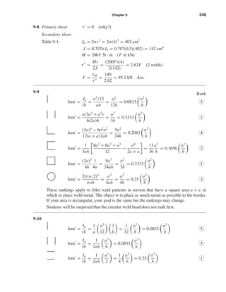
250. 250 Solutions Manual • Instructor’s Solution Manual to Accompany Mechanical Engineering Design
fom =
Iu
lh
=
1
[2(2a)]h
a2
6
(3a + a) =
1
6
a2
h
= 0.1667
a2
h
2
¯x =
b
2
=
a
2
, ¯y =
d2
b + 2d
=
a2
3a
=
a
3
Iu =
2d3
3
− 2d2 a
3
+ (b + 2d)
a2
9
=
2a3
3
−
2a3
3
+ 3a
a2
9
=
a3
3
fom =
Iu
lh
=
a3
/3
3ah
=
1
9
a2
h
= 0.1111
a2
h
4
Iu = πr3
=
πa3
8
fom =
Iu
lh
=
πa3
/8
πah
=
a2
8h
= 0.125
a2
h
3
The CEE-section pattern was not ranked because the deflection of the beam is out-of-plane.
If you have a square area in which to place a fillet weldment pattern under bending, your
objective is to place as much material as possible away from the x-axis. If your area is rec-
tangular, your goal is the same, but the rankings may change.
9-11 Materials:
Attachment (1018 HR) Sy = 32 kpsi, Sut = 58 kpsi
Member (A36) Sy = 36 kpsi, Sut ranges from 58 to 80 kpsi, use 58.
The member and attachment are weak compared to the E60XX electrode.
Decision Specify E6010 electrode
Controlling property: τall = min[0.3(58), 0.4(32)] = min(16.6, 12.8) = 12.8 kpsi
For a static load the parallel and transverse fillets are the same. If n is the number of beads,
τ =
F
n(0.707)hl
= τall
nh =
F
0.707lτall
=
25
0.707(3)(12.8)
= 0.921
Make a table.
Number of beads Leg size
n h
1 0.921
2 0.460 →1/2"
3 0.307 →5/16"
4 0.230 →1/4"
Decision: Specify 1/4" leg size
Decision: Weld all-around
shi20396_ch09.qxd 8/19/03 9:30 AM Page 250

251. Chapter 9 251
Weldment Specifications:
Pattern: All-around square
Electrode: E6010
Type: Two parallel fillets Ans.
Two transverse fillets
Length of bead: 12 in
Leg: 1/4 in
For a figure of merit of, in terms of weldbead volume, is this design optimal?
9-12 Decision: Choose a parallel fillet weldment pattern. By so-doing, we’ve chosen an optimal
pattern (see Prob. 9-9) and have thus reduced a synthesis problem to an analysis problem:
Table 9-1: A = 1.414hd = 1.414(h)(3) = 4.24h in3
Primary shear
τy =
V
A
=
3000
4.24h
=
707
h
Secondary shear
Table 9-1: Ju =
d(3b2
+ d2
)
6
=
3[3(32
) + 32
]
6
= 18 in3
J = 0.707(h)(18) = 12.7h in4
τx =
Mry
J
=
3000(7.5)(1.5)
12.7h
=
2657
h
= τy
τmax = τ 2
x + (τy + τy )2 =
1
h
26572 + (707 + 2657)2 =
4287
h
Attachment (1018 HR): Sy = 32 kpsi, Sut = 58 kpsi
Member (A36): Sy = 36 kpsi
The attachment is weaker
Decision: Use E60XX electrode
τall = min[0.3(58), 0.4(32)] = 12.8 kpsi
τmax = τall =
4287
h
= 12 800 psi
h =
4287
12 800
= 0.335 in
Decision: Specify 3/8" leg size
Weldment Specifications:
Pattern: Parallel fillet welds
Electrode: E6010
Type: Fillet Ans.
Length of bead: 6 in
Leg size: 3/8 in
shi20396_ch09.qxd 8/19/03 9:30 AM Page 251

252. 252 Solutions Manual • Instructor’s Solution Manual to Accompany Mechanical Engineering Design
9-13 An optimal square space (3" × 3") weldment pattern is ԽԽ or or ᮀ. In Prob. 9-12, there
was roundup of leg size to3/8 in. Consider the member material to be structural A36 steel.
Decision: Use a parallel horizontal weld bead pattern for welding optimization and
convenience.
Materials:
Attachment (1018 HR): Sy = 32 kpsi, Sut = 58 kpsi
Member (A36): Sy = 36 kpsi, Sut 58–80 kpsi; use 58 kpsi
From Table 9-4 AISC welding code,
τall = min[0.3(58), 0.4(32)] = min(16.6, 12.8) = 12.8 kpsi
Select a stronger electrode material from Table 9-3.
Decision: Specify E6010
Throat area and other properties:
A = 1.414hd = 1.414(h)(3) = 4.24h in2
¯x = b/2 = 3/2 = 1.5 in
¯y = d/2 = 3/2 = 1.5 in
Ju =
d(3b2
+ d2
)
6
=
3[3(32
) + 32
]
6
= 18 in3
J = 0.707hJu = 0.707(h)(18) = 12.73h in4
Primary shear:
τx =
V
A
=
3000
4.24h
=
707.5
h
Secondary shear:
τ =
Mr
J
τx = τ cos 45◦
=
Mr
J
cos 45◦
=
Mrx
J
τx =
3000(6 + 1.5)(1.5)
12.73h
=
2651
h
τy = τx =
2651
h
ry
x
rx
r ␶ЈЈ
␶ЈЈ
␶Ј
y
x
x
␶ЈЈy
shi20396_ch09.qxd 8/19/03 9:30 AM Page 252

253. Chapter 9 253
τmax = (τx + τx)2 + τ 2
y
=
1
h
(2651 + 707.5)2 + 26512
=
4279
h
psi
Relate stress and strength:
τmax = τall
4279
h
= 12 800
h =
4279
12 800
= 0.334 in → 3/8 in
Weldment Specifications:
Pattern: Horizontal parallel weld tracks
Electrode: E6010
Type of weld: Two parallel fillet welds
Length of bead: 6 in
Leg size: 3/8 in
Additional thoughts:
Since the round-up in leg size was substantial, why not investigate a backward C weld
pattern. One might then expect shorter horizontal weld beads which will have the advan-
tage of allowing a shorter member (assuming the member has not yet been designed). This
will show the inter-relationship between attachment design and supporting members.
9-14 Materials:
Member (A36): Sy = 36 kpsi, Sut = 58 to 80 kpsi; use Sut = 58 kpsi
Attachment (1018 HR): Sy = 32 kpsi, Sut = 58 kpsi
τall = min[0.3(58), 0.4(32)] = 12.8 kpsi
Decision: Use E6010 electrode. From Table 9-3: Sy = 50 kpsi, Sut = 62 kpsi,
τall = min[0.3(62), 0.4(50)] = 20 kpsi
Decision: Since A36 and 1018 HR are weld metals to an unknown extent, use
τall = 12.8 kpsi
Decision: Usethemostefficientweldpattern–square,weld-all-around.Choose6" × 6" size.
Attachment length:
l1 = 6 + a = 6 + 6.25 = 12.25 in
Throat area and other properties:
A = 1.414h(b + d) = 1.414(h)(6 + 6) = 17.0h
¯x =
b
2
=
6
2
= 3 in, ¯y =
d
2
=
6
2
= 3 in
shi20396_ch09.qxd 8/19/03 9:30 AM Page 253

254. 254 Solutions Manual • Instructor’s Solution Manual to Accompany Mechanical Engineering Design
Primary shear
τy =
V
A
=
F
A
=
20 000
17h
=
1176
h
psi
Secondary shear
Ju =
(b + d)3
6
=
(6 + 6)3
6
= 288 in3
J = 0.707h(288) = 203.6h in4
τx = τy =
Mry
J
=
20 000(6.25 + 3)(3)
203.6h
=
2726
h
psi
τmax = τ 2
x + (τy + τy)2 =
1
h
27262 + (2726 + 1176)2 =
4760
h
psi
Relate stress to strength
τmax = τall
4760
h
= 12 800
h =
4760
12 800
= 0.372 in
Decision:
Specify 3/8 in leg size
Specifications:
Pattern: All-around square weld bead track
Electrode: E6010
Type of weld: Fillet
Weld bead length: 24 in
Leg size: 3/8 in
Attachment length: 12.25 in
9-15 This is a good analysis task to test the students’ understanding
(1) Solicit information related to a priori decisions.
(2) Solicit design variables b and d.
(3) Find h and round and output all parameters on a single screen. Allow return to Step 1
or Step 2
(4) When the iteration is complete, the final display can be the bulk of your adequacy
assessment.
Such a program can teach too.
9-16 The objective of this design task is to have the students teach themselves that the weld
patterns of Table 9-3 can be added or subtracted to obtain the properties of a comtem-
plated weld pattern. The instructor can control the level of complication. I have left the
shi20396_ch09.qxd 8/19/03 9:30 AM Page 254

255. Chapter 9 255
presentation of the drawing to you. Here is one possibility. Study the problem’s opportuni-
ties, then present this (or your sketch) with the problem assignment.
Use b1 as the design variable. Express properties as a function of b1 . From Table 9-3,
category 3:
A = 1.414h(b − b1)
¯x = b/2, ¯y = d/2
Iu =
bd2
2
−
b1d2
2
=
(b − b1)d2
2
I = 0.707hIu
τ =
V
A
=
F
1.414h(b − b1)
τ =
Mc
I
=
Fa(d/2)
0.707hIu
τmax = τ 2 + τ 2
Parametric study
Let a = 10 in, b = 8 in, d = 8 in, b1 = 2 in, τall = 12.8 kpsi, l = 2(8 − 2) = 12 in
A = 1.414h(8 − 2) = 8.48h in2
Iu = (8 − 2)(82
/2) = 192 in3
I = 0.707(h)(192) = 135.7h in4
τ =
10 000
8.48h
=
1179
h
psi
τ =
10 000(10)(8/2)
135.7h
=
2948
h
psi
τmax =
1
h
11792 + 29482 =
3175
h
= 12 800
from which h = 0.248 in. Do not round off the leg size – something to learn.
fom =
Iu
hl
=
192
0.248(12)
= 64.5
A = 8.48(0.248) = 2.10 in2
I = 135.7(0.248) = 33.65 in4
Section AA
A36
Body welds
not shown
8"
8"
1
2
"
a
A
A
10000 lbf
1018 HR
Attachment weld
pattern considered
b
b1
d
shi20396_ch09.qxd 8/19/03 9:30 AM Page 255

256. 256 Solutions Manual • Instructor’s Solution Manual to Accompany Mechanical Engineering Design
vol =
h2
2
l =
0.2482
2
12 = 0.369 in3
I
vol
=
33.65
0.369
= 91.2 = eff
τ =
1179
0.248
= 4754 psi
τ =
2948
0.248
= 11 887 psi
τmax =
4127
0.248
.
= 12 800 psi
Now consider the case of uninterrupted welds,
b1 = 0
A = 1.414(h)(8 − 0) = 11.31h
Iu = (8 − 0)(82
/2) = 256 in3
I = 0.707(256)h = 181h in4
τ =
10 000
11.31h
=
884
h
τ =
10 000(10)(8/2)
181h
=
2210
h
τmax =
1
h
8842 + 22102 =
2380
h
= τall
h =
τmax
τall
=
2380
12 800
= 0.186 in
Do not round off h.
A = 11.31(0.186) = 2.10 in2
I = 181(0.186) = 33.67
τ =
884
0.186
= 4753 psi, vol =
0.1862
2
16 = 0.277 in3
τ =
2210
0.186
= 11 882 psi
fom =
Iu
hl
=
256
0.186(16)
= 86.0
eff =
I
(h2/2)l
=
33.67
(0.1862/2)16
= 121.7
Conclusions: To meet allowable stress limitations, I and A do not change, nor do τ and σ. To
meet the shortened bead length, h is increased proportionately. However, volume of bead laid
down increases as h2
. The uninterrupted bead is superior. In this example, we did not round h
and as a result we learned something. Our measures of merit are also sensitive to rounding.
When the design decision is made, rounding to the next larger standard weld fillet size will
decrease the merit.
shi20396_ch09.qxd 8/19/03 9:30 AM Page 256

257. Chapter 9 257
Had the weld bead gone around the corners, the situation would change. Here is a fol-
lowup task analyzing an alternative weld pattern.
9-17 From Table 9-2
For the box A = 1.414h(b + d)
Subtracting b1 from b and d1 from d
A = 1.414 h(b − b1 + d − d1)
Iu =
d2
6
(3b + d) −
d3
1
6
−
b1d2
2
=
1
2
(b − b1)d2
+
1
6
d3
− d3
1
length of bead l = 2(b − b1 + d − d1)
fom = Iu/hl
9-18 Below is a Fortran interactive program listing which, if imitated in any computer language
of convenience, will reduce to drudgery. Furthermore, the program allows synthesis by in-
teraction or learning without fatigue.
C Weld2.f for rect. fillet beads resisting bending C. Mischke Oct 98
1 print*,’weld2.f rectangular fillet weld-beads in bending,’
print*,’gaps allowed - C. Mischke Oct. 98’
print*,’ ’
print*,’Enter largest permissible shear stress tauall’
read*,tauall
print*,’Enter force F and clearance a’
read*,F,a
2 print*,’Enter width b and depth d of rectangular pattern’
read*,b,d
xbar=b/2.
ybar=d/2.
3 print*,’Enter width of gap b1, and depth of gap d1’
print*,’both gaps central in their respective sides’
read*,b1,d1
xIu=(b-b1)*d**2/2.+(d**3-d1**3)/6.
xl=2.*(d-d1)+2.*(b-b1)
b
b1
dd1
shi20396_ch09.qxd 8/19/03 9:30 AM Page 257

258. 258 Solutions Manual • Instructor’s Solution Manual to Accompany Mechanical Engineering Design
C Following calculations based on unit leg h = 1
AA=1.414*(b-b1+d-d1)
xI=0.707*xIu
tau2=F*a*d/2./xI
tau1=F/AA
taumax=sqrt(tau2**2+tau1**2)
h=taumax/tauall
C Adjust parameters for now-known h
AA=AA*h
xI=xI*h
tau2=tau2/h
tau1=tau1/h
taumax=taumax/h
fom=xIu/h/xl
print*,’F=’,F,’ a=’,a,’ bead length = ’,xl
print*,’b=’,b,’ b1=’,b1,’ d=’,d,’ d1=’,d1
print*,’xbar=’,xbar,’ ybar=’,ybar,’ Iu=’,xIu
print*,’I=’,xI,’ tau2=’,tau2,’ tau1=’,tau1
print*,’taumax=’,taumax,’ h=’,h,’ A=’,AA
print*,’fom=’,fom, ’I/(weld volume)=’,2.*xI/h**2/xl
print*,’ ’
print*,’To change b1,d1: 1; b,d: 2; New: 3; Quit: 4’
read*,index
go to (3,2,1,4), index
4 call exit
end
9-19 τall = 12 800 psi. Use Fig. 9-17(a) for general geometry, but employ beads and then ԽԽ
beads.
Horizontal parallel weld bead pattern
b = 6 in
d = 8 in
From Table 9-2, category 3
A = 1.414 hb = 1.414(h)(6) = 8.48 h in2
¯x = b/2 = 6/2 = 3 in, ¯y = d/2 = 8/2 = 4 in
Iu =
bd2
2
=
6(8)2
2
= 192 in3
I = 0.707hIu = 0.707(h)(192) = 135.7h in4
τ =
10 000
8.48h
=
1179
h
psi
6"
8"
shi20396_ch09.qxd 8/19/03 9:30 AM Page 258

259. Chapter 9 259
τ =
Mc
I
=
10 000(10)(8/2)
135.7h
=
2948
h
psi
τmax = τ 2 + τ 2 =
1
h
(11792
+ 29482
)1/2
=
3175
h
psi
Equate the maximum and allowable shear stresses.
τmax = τall =
3175
h
= 12 800
from which h = 0.248 in. It follows that
I = 135.7(0.248) = 33.65 in4
The volume of the weld metal is
vol =
h2
l
2
=
0.2482
(6 + 6)
2
= 0.369 in3
The effectiveness, (eff)H , is
(eff)H =
I
vol
=
33.65
0.369
= 91.2 in
(fom )H =
Iu
hl
=
192
0.248(6 + 6)
= 64.5 in
Vertical parallel weld beads
b = 6 in
d = 8 in
From Table 9-2, category 2
A = 1.414hd = 1.414(h)(8) = 11.31h in2
¯x = b/2 = 6/2 = 3 in, ¯y = d/2 = 8/2 = 4 in
Iu =
d3
6
=
83
6
= 85.33 in3
I = 0.707hIu = 0.707(h)(85.33) = 60.3h
τ =
10 000
11.31h
=
884
h
psi
τ =
Mc
I
=
10 000(10)(8/2)
60.3 h
=
6633
h
psi
τmax = τ 2 + τ 2 =
1
h
(8842
+ 66332
)1/2
=
6692
h
psi
8"
6"
shi20396_ch09.qxd 8/19/03 9:30 AM Page 259

260. 260 Solutions Manual • Instructor’s Solution Manual to Accompany Mechanical Engineering Design
Equating τmax to τall gives h = 0.523 in. It follows that
I = 60.3(0.523) = 31.5 in4
vol =
h2
l
2
=
0.5232
2
(8 + 8) = 2.19 in3
(eff)V =
I
vol
=
31.6
2.19
= 14.4 in
(fom )V =
Iu
hl
=
85.33
0.523(8 + 8)
= 10.2 in
The ratio of (eff)V/(eff)H is 14.4/91.2 = 0.158. The ratio (fom )V/(fom )H is
10.2/64.5 = 0.158. This is not surprising since
eff =
I
vol
=
I
(h2/2)l
=
0.707 hIu
(h2/2)l
= 1.414
Iu
hl
= 1.414 fom
The ratios (eff)V/(eff)H and (fom )V/(fom )H give the same information.
9-20 Because the loading is pure torsion, there is no primary shear. From Table 9-1, category 6:
Ju = 2πr3
= 2π(1)3
= 6.28 in3
J = 0.707 hJu = 0.707(0.25)(6.28)
= 1.11 in4
τ =
Tr
J
=
20(1)
1.11
= 18.0 kpsi Ans.
9-21 h = 0.375 in, d = 8 in, b = 1 in
From Table 9-2, category 2:
A = 1.414(0.375)(8) = 4.24 in2
Iu =
d3
6
=
83
6
= 85.3 in3
I = 0.707hIu = 0.707(0.375)(85.3) = 22.6 in4
τ =
F
A
=
5
4.24
= 1.18 kpsi
M = 5(6) = 30 kip · in
c = (1 + 8 + 1 − 2)/2 = 4 in
τ =
Mc
I
=
30(4)
22.6
= 5.31 kpsi
τmax = τ 2 + τ 2 = 1.182 + 5.312
= 5.44 kpsi Ans.
shi20396_ch09.qxd 8/19/03 9:30 AM Page 260

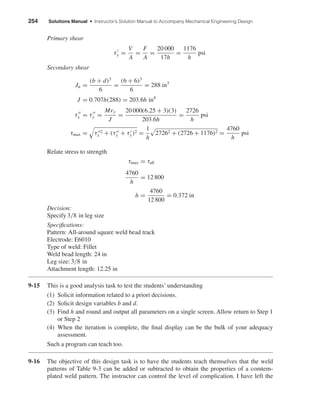
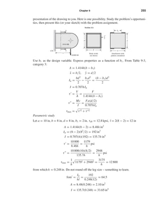
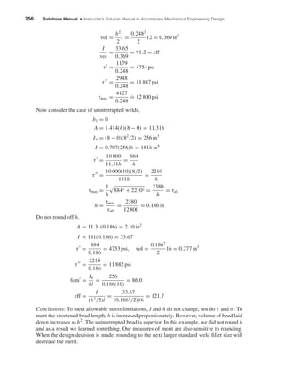
261. Chapter 9 261
9-22 h = 0.6 cm, b = 6 cm, d = 12 cm.
Table 9-3, category 5:
A = 0.707h(b + 2d)
= 0.707(0.6)[6 + 2(12)] = 12.7 cm2
¯y =
d2
b + 2d
=
122
6 + 2(12)
= 4.8 cm
Iu =
2d3
3
− 2d2
¯y + (b + 2d) ¯y2
=
2(12)3
3
− 2(122
)(4.8) + [6 + 2(12)]4.82
= 461 cm3
I = 0.707hIu = 0.707(0.6)(461) = 196 cm4
τ =
F
A
=
7.5(103)
12.7(102)
= 5.91 MPa
M = 7.5(120) = 900 N · m
cA = 7.2 cm, cB = 4.8 cm
The critical location is at A.
τA =
McA
I
=
900(7.2)
196
= 33.1 MPa
τmax = τ 2 + τ 2 = (5.912
+ 33.12
)1/2
= 33.6 MPa
n =
τall
τmax
=
120
33.6
= 3.57 Ans.
9-23 The largest possible weld size is 1/16 in. This is a small weld and thus difficult to accom-
plish. The bracket’s load-carrying capability is not known. There are geometry problems
associated with sheet metal folding, load-placement and location of the center of twist.
This is not available to us. We will identify the strongest possible weldment.
Use a rectangular, weld-all-around pattern – Table 9-2, category 6:
A = 1.414 h(b + d)
= 1.414(1/16)(1 + 7.5)
= 0.751 in2
¯x = b/2 = 0.5 in
¯y =
d
2
=
7.5
2
= 3.75 in
6
4.8
7.2
A
B
G
1"
7.5"
shi20396_ch09.qxd 8/19/03 9:30 AM Page 261

262. 262 Solutions Manual • Instructor’s Solution Manual to Accompany Mechanical Engineering Design
Iu =
d2
6
(3b + d) =
7.52
6
[3(1) + 7.5] = 98.4 in3
I = 0.707hIu = 0.707(1/16)(98.4) = 4.35 in4
M = (3.75 + 0.5)W = 4.25W
τ =
V
A
=
W
0.751
= 1.332W
τ =
Mc
I
=
4.25W(7.5/2)
4.35
= 3.664W
τmax = τ 2 + τ 2 = W 1.3322 + 3.6642 = 3.90W
Material properties: The allowable stress given is low. Let’s demonstrate that.
For the A36 structural steel member, Sy = 36 kpsi and Sut = 58 kpsi. For the 1020 CD
attachment, use HR properties of Sy = 30 kpsi and Sut = 55. The E6010 electrode has
strengths of Sy = 50 and Sut = 62 kpsi.
Allowable stresses:
A36: τall = min[0.3(58), 0.4(36)]
= min(17.4, 14.4) = 14.4 kpsi
1020: τall = min[0.3(55), 0.4(30)]
τall = min(16.5, 12) = 12 kpsi
E6010: τall = min[0.3(62), 0.4(50)]
= min(18.6, 20) = 18.6 kpsi
Since Table 9-6 gives 18.0 kpsi as the allowable shear stress, use this lower value.
Therefore, the allowable shear stress is
τall = min(14.4, 12, 18.0) = 12 kpsi
However, the allowable stress in the problem statement is 0.9 kpsi which is low from the
weldment perspective. The load associated with this strength is
τmax = τall = 3.90W = 900
W =
900
3.90
= 231 lbf
If the welding can be accomplished (1/16 leg size is a small weld), the weld strength is
12 000 psi and the load W = 3047 lbf. Can the bracket carry such a load?
There are geometry problems associated with sheet metal folding. Load placement is
important and the center of twist has not been identified. Also, the load-carrying capability
of the top bend is unknown.
These uncertainties may require the use of a different weld pattern. Our solution pro-
vides the best weldment and thus insight for comparing a welded joint to one which em-
ploys screw fasteners.
shi20396_ch09.qxd 8/19/03 9:30 AM Page 262

263. Chapter 9 263
9-24
F = 100 lbf, τall = 3 kpsi
FB = 100(16/3) = 533.3 lbf
Fx
B = −533.3 cos 60◦
= −266.7 lbf
F
y
B = −533.3 cos 30◦
= −462 lbf
It follows that R
y
A = 562 lbf and Rx
A = 266.7 lbf, RA = 622 lbf
M = 100(16) = 1600 lbf · in
The OD of the tubes is 1 in. From Table 9-1, category 6:
A = 1.414(πhr)(2)
= 2(1.414)(πh)(1/2) = 4.44h in2
Ju = 2πr3
= 2π(1/2)3
= 0.785 in3
J = 2(0.707)hJu = 1.414(0.785)h = 1.11h in4
τ =
V
A
=
622
4.44h
=
140
h
τ =
Tc
J
=
Mc
J
=
1600(0.5)
1.11h
=
720.7
h
The shear stresses, τ and τ , are additive algebraically
τmax =
1
h
(140 + 720.7) =
861
h
psi
τmax = τall =
861
h
= 3000
h =
861
3000
= 0.287 → 5/16"
Decision: Use 5/16 in fillet welds Ans.
100
16
3
562
266.7
266.7
462
F
FB
B
A
R
x
A
R
y
A
60Њ
y
x
shi20396_ch09.qxd 8/19/03 9:30 AM Page 263

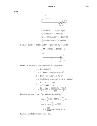
264. 264 Solutions Manual • Instructor’s Solution Manual to Accompany Mechanical Engineering Design
9-25
For the pattern in bending shown, find the centroid G of the weld group.
¯x =
6(0.707)(1/4)(3) + 6(0.707)(3/8)(13)
6(0.707)(1/4) + 6(0.707)(3/8)
= 9 in
I1/4 = 2 IG + A2
¯x
= 2
0.707(1/4)(63
)
12
+ 0.707(1/4)(6)(62
)
= 82.7 in4
I3/8 = 2
0.707(3/8)(63
)
12
+ 0.707(3/8)(6)(42
)
= 60.4 in4
I = I1/4 + I3/8 = 82.7 + 60.4 = 143.1 in4
The critical location is at B. From Eq. (9-3),
τ =
F
2[6(0.707)(3/8 + 1/4)]
= 0.189F
τ =
Mc
I
=
(8F)(9)
143.1
= 0.503F
τmax = τ 2 + τ 2 = F 0.1892 + 0.5032 = 0.537F
Materials:
A36 Member: Sy = 36 kpsi
1015 HR Attachment: Sy = 27.5 kpsi
E6010 Electrode: Sy = 50 kpsi
τall = 0.577 min(36, 27.5, 50) = 15.9 kpsi
F =
τall/n
0.537
=
15.9/2
0.537
= 14.8 kip Ans.
9-26 Figure P9-26b is a free-body diagram of the bracket. Forces and moments that act on the
welds are equal, but of opposite sense.
(a) M = 1200(0.366) = 439 lbf · in Ans.
(b) Fy = 1200 sin 30◦
= 600 lbf Ans.
(c) Fx = 1200 cos 30◦
= 1039 lbf Ans.
3
8
"
3
8
"
1
4
"
1
4
"
7"9"
g
g
g
g
y
x
G
B
shi20396_ch09.qxd 8/19/03 9:30 AM Page 264

265. Chapter 9 265
(d) From Table 9-2, category 6:
A = 1.414(0.25)(0.25 + 2.5) = 0.972 in2
Iu =
d2
6
(3b + d) =
2.52
6
[3(0.25) + 2.5] = 3.39 in3
The second area moment about an axis through G and parallel to z is
I = 0.707hIu = 0.707(0.25)(3.39) = 0.599 in4
Ans.
(e) Refer to Fig. P.9-26b. The shear stress due to Fy is
τ1 =
Fy
A
=
600
0.972
= 617 psi
The shear stress along the throat due to Fx is
τ2 =
Fx
A
=
1039
0.972
= 1069 psi
The resultant of τ1 and τ2 is in the throat plane
τ = τ2
1 + τ2
2
1/2
= (6172
+ 10692
)1/2
= 1234 psi
The bending of the throat gives
τ =
Mc
I
=
439(1.25)
0.599
= 916 psi
The maximum shear stress is
τmax = (τ 2
+ τ 2
)1/2
= (12342
+ 9162
)1/2
= 1537 psi Ans.
(f) Materials:
1018 HR Member: Sy = 32 kpsi, Sut = 58 kpsi (Table A-20)
E6010 Electrode: Sy = 50 kpsi (Table 9-3)
n =
Ssy
τmax
=
0.577Sy
τmax
=
0.577(32)
1.537
= 12.0 Ans.
(g) Bending in the attachment near the base. The cross-sectional area is approximately
equal to bh.
A1
.
= bh = 0.25(2.5) = 0.625 in2
τxy =
Fx
A1
=
1039
0.625
= 1662 psi
I
c
=
bd2
6
=
0.25(2.5)2
6
= 0.260 in3
At location A
σy =
Fy
A1
+
M
I/c
σy =
600
0.625
+
439
0.260
= 2648 psi
shi20396_ch09.qxd 8/19/03 9:30 AM Page 265

266. 266 Solutions Manual • Instructor’s Solution Manual to Accompany Mechanical Engineering Design
The von Mises stress σ is
σ = σ2
y + 3τ2
xy
1/2
= [26482
+ 3(1662)2
]1/2
= 3912 psi
Thus, the factor of safety is,
n =
Sy
σ
=
32
3.912
= 8.18 Ans.
The clip on the mooring line bears against the side of the 1/2-in hole. If the clip fills
the hole
σ =
F
td
=
−1200
0.25(0.50)
= −9600 psi
n = −
Sy
σ
= −
32(103
)
−9600
= 3.33 Ans.
Further investigation of this situation requires more detail than is included in the task
statement.
(h) In shear fatigue, the weakest constituent of the weld melt is 1018 with Sut = 58 kpsi
Se = 0.504Sut = 0.504(58) = 29.2 kpsi
Table 7-4:
ka = 14.4(58)−0.718
= 0.780
For the size factor estimate, we first employ Eq. (7-24) for the equivalent diameter.
de = 0.808
√
0.707hb = 0.808 0.707(2.5)(0.25) = 0.537 in
Eq. (7-19) is used next to find kb
kb =
de
0.30
−0.107
=
0.537
0.30
−0.107
= 0.940
The load factor for shear kc , is
kc = 0.59
The endurance strength in shear is
Sse = 0.780(0.940)(0.59)(29.2) = 12.6 kpsi
From Table 9-5, the shear stress-concentration factor is Kf s = 2.7. The loading is
repeatedly-applied.
τa = τm = kf
τmax
2
= 2.7
1.537
2
= 2.07 kpsi
Table 7-10: Gerber factor of safety nf , adjusted for shear, with Ssu = 0.67Sut
nf =
1
2
0.67(58)
2.07
2
2.07
12.6



−1 + 1 +
2(2.07)(12.6)
0.67(58)(2.07)
2



= 5.55 Ans.
Attachment metal should be checked for bending fatigue.
shi20396_ch09.qxd 8/19/03 9:30 AM Page 266

267. Chapter 9 267
9-27 Use b = d = 4 in. Since h = 5/8 in, the primary shear is
τ =
F
1.414(5/8)(4)
= 0.283F
The secondary shear calculations, for a moment arm of 14 in give
Ju =
4[3(42
) + 42
]
6
= 42.67 in3
J = 0.707hJu = 0.707(5/8)42.67 = 18.9 in4
τx = τy =
Mry
J
=
14F(2)
18.9
= 1.48F
Thus, the maximum shear and allowable load are:
τmax = F 1.482 + (0.283 + 1.48)2 = 2.30F
F =
τall
2.30
=
20
2.30
= 8.70 kip Ans.
From Prob. 9-5b, τall = 11 kpsi
Fall =
τall
2.30
=
11
2.30
= 4.78 kip
The allowable load has thus increased by a factor of 1.8 Ans.
9-28 Purchase the hook having the design shown in Fig. P9-28b. Referring to text Fig. 9-32a,
this design reduces peel stresses.
9-29 (a)
¯τ =
1
l
l/2
−l/2
Pω cosh(ωx)
4b sinh(ωl/2)
dx
= A1
l/2
−l/2
cosh(ωx) dx
=
A1
ω
sinh(ωx)
l/2
−l/2
=
A1
ω
[sinh(ωl/2) − sinh(−ωl/2)]
=
A1
ω
[sinh(ωl/2) − (−sinh(ωl/2))]
=
2A1 sinh(ωl/2)
ω
=
Pω
4bl sinh(ωl/2)
[2 sinh(ωl/2)]
¯τ =
P
2bl
Ans.
shi20396_ch09.qxd 8/19/03 9:30 AM Page 267

268. 268 Solutions Manual • Instructor’s Solution Manual to Accompany Mechanical Engineering Design
(b) τ(l/2) =
Pω cosh(ωl/2)
4b sinh(ωl/2)
=
Pω
4b tanh(ωl/2)
Ans.
(c)
K =
τ(l/2)
¯τ
=
Pω
4b sinh(ωl/2)
2bl
P
K =
ωl/2
tanh(ωl/2)
Ans.
For computer programming, it can be useful to express the hyperbolic tangent in terms
of exponentials:
K =
ωl
2
exp(ωl/2) − exp(−ωl/2)
exp(ωl/2) + exp(−ωl/2)
Ans.
9-30 This is a computer programming exercise. All programs will vary.
shi20396_ch09.qxd 8/19/03 9:30 AM Page 268

269. Chapter 10
10-1
10-2 A = Sdm
dim(Auscu) = dim(S) dim(dm
) = kpsi · inm
dim(ASI) = dim(S1) dim dm
1 = MPa · mmm
ASI =
MPa
kpsi
·
mmm
inm Auscu = 6.894 757(25.40)m
Auscu
.
= 6.895(25.4)m
Auscu Ans.
For music wire, from Table 10-4:
Auscu = 201, m = 0.145; what is ASI?
ASI = 6.89(25.4)0.145
(201) = 2214 MPa · mmm
Ans.
10-3 Given: Music wire, d = 0.105 in, OD = 1.225 in, plain ground ends, Nt = 12 coils.
Table 10-1: Na = Nt − 1 = 12 − 1 = 11
Ls = dNt = 0.105(12) = 1.26 in
Table 10-4: A = 201, m = 0.145
(a) Eq. (10-14): Sut =
201
(0.105)0.145
= 278.7 kpsi
Table 10-6: Ssy = 0.45(278.7) = 125.4 kpsi
D = 1.225 − 0.105 = 1.120 in
C =
D
d
=
1.120
0.105
= 10.67
Eq. (10-6): KB =
4(10.67) + 2
4(10.67) − 3
= 1.126
Eq. (10-3): F|Ssy
=
πd3
Ssy
8KB D
=
π(0.105)3
(125.4)(103
)
8(1.126)(1.120)
= 45.2 lbf
Eq. (10-9): k =
d4
G
8D3 Na
=
(0.105)4
(11.75)(106
)
8(1.120)3(11)
= 11.55 lbf/in
L0 =
F|Ssy
k
+ Ls =
45.2
11.55
+ 1.26 = 5.17 in Ans.
1
2
"
4"
1"
1
2
"
4"
1"
shi20396_ch10.qxd 8/11/03 4:39 PM Page 269

270. 270 Solutions Manual • Instructor’s Solution Manual to Accompany Mechanical Engineering Design
(b) F|Ssy
= 45.2 lbf Ans.
(c) k = 11.55 lbf/in Ans.
(d) (L0)cr =
2.63D
α
=
2.63(1.120)
0.5
= 5.89 in
Many designers provide (L0)cr/L0 ≥ 5 or more; therefore, plain ground ends are not
often used in machinery due to buckling uncertainty.
10-4 Referring to Prob. 10-3 solution, C = 10.67, Na = 11, Ssy = 125.4 kpsi, (L0)cr =
5.89 in and F = 45.2 lbf (at yield).
Eq. (10-18): 4 ≤ C ≤ 12 C = 10.67 O.K.
Eq. (10-19): 3 ≤ Na ≤ 15 Na = 11 O.K.
L0 = 5.17 in, Ls = 1.26 in
y1 =
F1
k
=
30
11.55
= 2.60 in
L1 = L0 − y1 = 5.17 − 2.60 = 2.57 in
ξ =
ys
y1
− 1 =
5.17 − 1.26
2.60
− 1 = 0.50
Eq. (10-20): ξ ≥ 0.15, ξ = 0.50 O.K.
From Eq. (10-3) for static service
τ1 = KB
8F1 D
πd3
= 1.126
8(30)(1.120)
π(0.105)3
= 83 224 psi
ns =
Ssy
τ1
=
125.4(103
)
83 224
= 1.51
Eq. (10-21): ns ≥ 1.2, ns = 1.51 O.K.
τs = τ1
45.2
30
= 83 224
45.2
30
= 125 391 psi
Ssy/τs = 125.4(103
)/125 391
.
= 1
Ssy/τs ≥ (ns)d: Not solid-safe. Not O.K.
L0 ≤ (L0)cr: 5.17 ≤ 5.89 Margin could be higher, Not O.K.
Design is unsatisfactory. Operate over a rod? Ans.
L0
L1
y1 F1
ys
Ls
Fs
shi20396_ch10.qxd 8/11/03 4:39 PM Page 270

271. Chapter 10 271
10-5 Static service spring with: HD steel wire, d = 2 mm, OD = 22 mm, Nt = 8.5 turns plain
and ground ends.
Preliminaries
Table 10-5: A = 1783 MPa · mmm
, m = 0.190
Eq. (10-14): Sut =
1783
(2)0.190
= 1563 MPa
Table 10-6: Ssy = 0.45(1563) = 703.4 MPa
Then,
D = OD − d = 22 − 2 = 20 mm
C = 20/2 = 10
KB =
4C + 2
4C − 3
=
4(10) + 2
4(10) − 3
= 1.135
Na = 8.5 − 1 = 7.5 turns
Ls = 2(8.5) = 17 mm
Eq. (10-21): Use (ns)d = 1.2 for solid-safe property.
Fs =
πd3
Ssy/nd
8KB D
=
π(2)3
(703.4/1.2)
8(1.135)(20)
(10−3
)3
(106
)
10−3
= 81.12 N
k =
d4
G
8D3 Na
=
(2)4
(79.3)
8(20)3(7.5)
(10−3
)4
(109
)
(10−3)3
= 0.002 643(106
) = 2643 N/m
ys =
Fs
k
=
81.12
2643(10−3)
= 30.69 mm
(a) L0 = y + Ls = 30.69 + 17 = 47.7 mm Ans.
(b) Table 10-1: p =
L0
Nt
=
47.7
8.5
= 5.61 mm Ans.
(c) Fs = 81.12 N (from above) Ans.
(d) k = 2643 N/m (from above) Ans.
(e) Table 10-2 and Eq. (10-13):
(L0)cr =
2.63D
α
=
2.63(20)
0.5
= 105.2 mm
(L0)cr/L0 = 105.2/47.7 = 2.21
This is less than 5. Operate over a rod?
Plain and ground ends have a poor eccentric footprint. Ans.
10-6 Referring to Prob. 10-5 solution: C = 10, Na = 7.5, k = 2643 N/m, d = 2 mm,
D = 20 mm, Fs = 81.12 N and Nt = 8.5 turns.
Eq. (10-18): 4 ≤ C ≤ 12, C = 10 O.K.
shi20396_ch10.qxd 8/11/03 4:39 PM Page 271

272. 272 Solutions Manual • Instructor’s Solution Manual to Accompany Mechanical Engineering Design
Eq. (10-19): 3 ≤ Na ≤ 15, Na = 7.5 O.K.
y1 =
F1
k
=
75
2643(10−3)
= 28.4 mm
(y)for yield =
81.12(1.2)
2643(10−3)
= 36.8 mm
ys =
81.12
2643(10−3)
= 30.69 mm
ξ =
(y)for yield
y1
− 1 =
36.8
28.4
− 1 = 0.296
Eq. (10-20): ξ ≥ 0.15, ξ = 0.296 O.K.
Table 10-6: Ssy = 0.45Sut O.K.
As-wound
τs = KB
8Fs D
πd3
= 1.135
8(81.12)(20)
π(2)3
10−3
(10−3)3(106)
= 586 MPa
Eq. (10-21):
Ssy
τs
=
703.4
586
= 1.2 O.K. (Basis for Prob. 10-5 solution)
Table 10-1: Ls = Ntd = 8.5(2) = 17 mm
L0 =
Fs
k
+ Ls =
81.12
2.643
+ 17 = 47.7 mm
2.63D
α
=
2.63(20)
0.5
= 105.2 mm
(L0)cr
L0
=
105.2
47.7
= 2.21
which is less than 5. Operate over a rod? Not O.K.
Plain and ground ends have a poor eccentric footprint. Ans.
10-7 Given: A228 (music wire), SQ&GRD ends, d = 0.006 in, OD = 0.036 in, L0 = 0.63 in,
Nt = 40 turns.
Table 10-4: A = 201 kpsi · inm
, m = 0.145
D = OD − d = 0.036 − 0.006 = 0.030 in
C = D/d = 0.030/0.006 = 5
KB =
4(5) + 2
4(5) − 3
= 1.294
Table 10-1: Na = Nt − 2 = 40 − 2 = 38 turns
Sut =
201
(0.006)0.145
= 422.1 kpsi
Ssy = 0.45(422.1) = 189.9 kpsi
k =
Gd4
8D3 Na
=
12(106
)(0.006)4
8(0.030)3(38)
= 1.895 lbf/in
shi20396_ch10.qxd 8/11/03 4:39 PM Page 272

273. Chapter 10 273
Table 10-1: Ls = Ntd = 40(0.006) = 0.240 in
Now Fs = kys where ys = L0 − Ls = 0.390 in. Thus,
τs = KB
8(kys)D
πd3
= 1.294
8(1.895)(0.39)(0.030)
π(0.006)3
(10−3
) = 338.2 kpsi (1)
τs > Ssy , that is, 338.2 > 189.9 kpsi; the spring is not solid-safe. Solving Eq. (1) for ys
gives
ys =
(τs/n)(πd3
)
8KBkD
=
(189 900/1.2)(π)(0.006)3
8(1.294)(1.895)(0.030)
= 0.182 in
Using a design factor of 1.2,
L0 = Ls + ys = 0.240 + 0.182 = 0.422 in
The spring should be wound to a free length of 0.422 in. Ans.
10-8 Given: B159 (phosphor bronze), SQ&GRD ends, d = 0.012 in, OD = 0.120 in, L0 =
0.81 in, Nt = 15.1 turns.
Table 10-4: A = 145 kpsi · inm
, m = 0
Table 10-5: G = 6 Mpsi
D = OD − d = 0.120 − 0.012 = 0.108 in
C = D/d = 0.108/0.012 = 9
KB =
4(9) + 2
4(9) − 3
= 1.152
Table 10-1: Na = Nt − 2 = 15.1 − 2 = 13.1 turns
Sut =
145
0.0120
= 145 kpsi
Table 10-6: Ssy = 0.35(145) = 50.8 kpsi
k =
Gd4
8D3 Na
=
6(106
)(0.012)4
8(0.108)3(13.1)
= 0.942 lbf/in
Table 10-1: Ls = dNt = 0.012(15.1) = 0.181 in
Now Fs = kys , ys = L0 − Ls = 0.81 − 0.181 = 0.629 in
τs = KB
8(kys)D
πd3
= 1.152
8(0.942)(0.6)(0.108)
π(0.012)3
(10−3
) = 108.6 kpsi (1)
τs > Ssy , that is,108.6 > 50.8 kpsi; the spring is not solid safe. Solving Eq. (1) for ys gives
ys =
(Ssy/n)πd3
8KBkD
=
(50.8/1.2)(π)(0.012)3
(103
)
8(1.152)(0.942)(0.108)
= 0.245 in
L0 = Ls + ys = 0.181 + 0.245 = 0.426 in
Wind the spring to a free length of 0.426 in. Ans.
shi20396_ch10.qxd 8/11/03 4:39 PM Page 273

274. 274 Solutions Manual • Instructor’s Solution Manual to Accompany Mechanical Engineering Design
10-9 Given: A313 (stainless steel), SQ&GRD ends, d = 0.040 in, OD = 0.240 in, L0 =
0.75 in, Nt = 10.4 turns.
Table 10-4: A = 169 kpsi · inm
, m = 0.146
Table 10-5: G = 10(106
) psi
D = OD − d = 0.240 − 0.040 = 0.200 in
C = D/d = 0.200/0.040 = 5
KB =
4(5) + 2
4(5) − 3
= 1.294
Table 10-6: Na = Nt − 2 = 10.4 − 2 = 8.4 turns
Sut =
169
(0.040)0.146
= 270.4 kpsi
Table 10-13: Ssy = 0.35(270.4) = 94.6 kpsi
k =
Gd4
8D3 Na
=
10(106
)(0.040)4
8(0.2)3(8.4)
= 47.62 lbf/in
Table 10-6: Ls = dNt = 0.040(10.4) = 0.416 in
Now Fs = kys , ys = L0 − Ls = 0.75 − 0.416 = 0.334 in
τs = KB
8(kys)D
πd3
= 1.294
8(47.62)(0.334)(0.2)
π(0.040)3
(10−3
) = 163.8 kpsi (1)
τs > Ssy , that is,163.8 > 94.6 kpsi; the spring is not solid-safe. Solving Eq. (1) for ys gives
ys =
(Ssy/n)(πd3
)
8KBkD
=
(94 600/1.2)(π)(0.040)3
8(1.294)(47.62)(0.2)
= 0.161 in
L0 = Ls + ys = 0.416 + 0.161 = 0.577 in
Wind the spring to a free length 0.577 in. Ans.
10-10 Given: A227 (hard drawn steel), d = 0.135 in, OD = 2.0 in, L0 = 2.94 in, Nt = 5.25
turns.
Table 10-4: A = 140 kpsi · inm
, m = 0.190
Table 10-5: G = 11.4(106
) psi
D = OD − d = 2 − 0.135 = 1.865 in
C = D/d = 1.865/0.135 = 13.81
KB =
4(13.81) + 2
4(13.81) − 3
= 1.096
Na = Nt − 2 = 5.25 − 2 = 3.25 turns
Sut =
140
(0.135)0.190
= 204.8 kpsi
shi20396_ch10.qxd 8/11/03 4:39 PM Page 274

275. Chapter 10 275
Table 10-6: Ssy = 0.45(204.8) = 92.2 kpsi
k =
Gd4
8D3 Na
=
11.4(106
)(0.135)4
8(1.865)3(3.25)
= 22.45 lbf/in
Table 10-1: Ls = dNt = 0.135(5.25) = 0.709 in
Now Fs = kys , ys = L0 − Ls = 2.94 − 0.709 = 2.231 in
τs = KB
8(kys)D
πd3
= 1.096
8(22.45)(2.231)(1.865)
π(0.135)3
(10−3
) = 106.0 kpsi (1)
τs > Ssy , that is,106 > 92.2 kpsi; the spring is not solid-safe. Solving Eq. (1) for ys gives
ys =
(Ssy/n)(πd3
)
8KBkD
=
(92 200/1.2)(π)(0.135)3
8(1.096)(22.45)(1.865)
= 1.612 in
L0 = Ls + ys = 0.709 + 1.612 = 2.321 in
Wind the spring to a free length of 2.32 in. Ans.
10-11 Given: A229 (OQ&T steel), SQ&GRD ends, d = 0.144 in, OD = 1.0 in, L0 = 3.75 in,
Nt = 13 turns.
Table 10-4: A = 147 kpsi · inm
, m = 0.187
Table 10-5: G = 11.4(106
) psi
D = OD − d = 1.0 − 0.144 = 0.856 in
C = D/d = 0.856/0.144 = 5.944
KB =
4(5.944) + 2
4(5.944) − 3
= 1.241
Table 10-1: Na = Nt − 2 = 13 − 2 = 11 turns
Sut =
147
(0.144)0.187
= 211.2 kpsi
Table 10-6: Ssy = 0.50(211.2) = 105.6 kpsi
k =
Gd4
8D3 Na
=
11.4(106
)(0.144)4
8(0.856)3(11)
= 88.8 lbf/in
Table 10-1: Ls = dNt = 0.144(13) = 1.872 in
Now Fs = kys, ys = L0 − Ls = 3.75 − 1.872 = 1.878 in
τs = KB
8(kys)D
πd3
= 1.241
8(88.8)(1.878)(0.856)
π(0.144)3
(10−3
) = 151.1 kpsi (1)
τs > Ssy , that is,151.1 > 105.6 kpsi; the spring is not solid-safe. Solving Eq. (1) for ys gives
ys =
(Ssy/n)(πd3
)
8KBkD
=
(105 600/1.2)(π)(0.144)3
8(1.241)(88.8)(0.856)
= 1.094 in
L0 = Ls + ys = 1.878 + 1.094 = 2.972 in
Wind the spring to a free length 2.972 in. Ans.
shi20396_ch10.qxd 8/11/03 4:39 PM Page 275

276. 276 Solutions Manual • Instructor’s Solution Manual to Accompany Mechanical Engineering Design
10-12 Given: A232 (Cr-V steel), SQ&GRD ends, d = 0.192 in, OD = 3 in, L0 = 9 in, Nt =
8 turns.
Table 10-4: A = 169 kpsi · inm
, m = 0.168
Table 10-5: G = 11.2(106
) psi
D = OD − d = 3 − 0.192 = 2.808 in
C = D/d = 2.808/0.192 = 14.625
KB =
4(14.625) + 2
4(14.625) − 3
= 1.090
Table 10-1: Na = Nt − 2 = 8 − 2 = 6 turns
Sut =
169
(0.192)0.168
= 223.0 kpsi
Table 10-6: Ssy = 0.50(223.0) = 111.5 kpsi
k =
Gd4
8D3 Na
=
11.2(106
)(0.192)4
8(2.808)3(6)
= 14.32 lbf/in
Table 10-1: Ls = dNt = 0.192(8) = 1.536 in
Now Fs = kys, ys = L0 − Ls = 9 − 1.536 = 7.464 in
τs = KB
8(kys)D
πd3
= 1.090
8(14.32)(7.464)(2.808)
π(0.192)3
(10−3
) = 117.7 kpsi (1)
τs > Ssy, that is,117.7 > 111.5 kpsi; the spring is not solid safe. Solving Eq. (1) for ys gives
ys =
(Ssy/n)(πd3
)
8KBkD
=
(111 500/1.2)(π)(0.192)3
8(1.090)(14.32)(2.808)
= 5.892 in
L0 = Ls + ys = 1.536 + 5.892 = 7.428 in
Wind the spring to a free length of 7.428 in. Ans.
10-13 Given: A313 (stainless steel) SQ&GRD ends, d = 0.2 mm, OD = 0.91 mm, L0 =
15.9 mm, Nt = 40 turns.
Table 10-4: A = 1867 MPa · mmm
, m = 0.146
Table 10-5: G = 69.0 GPa
D = OD − d = 0.91 − 0.2 = 0.71 mm
C = D/d = 0.71/0.2 = 3.55
KB =
4(3.55) + 2
4(3.55) − 3
= 1.446
Na = Nt − 2 = 40 − 2 = 38 turns
Sut =
1867
(0.2)0.146
= 2361.5 MPa
shi20396_ch10.qxd 8/11/03 4:39 PM Page 276

277. Chapter 10 277
Table 10-6:
Ssy = 0.35(2361.5) = 826.5 MPa
k =
d4
G
8D3 Na
=
(0.2)4
(69.0)
8(0.71)3(38)
(10−3
)4
(109
)
(10−3)3
= 1.0147(10−3
)(106
) = 1014.7 N/m or 1.0147 N/mm
Ls = dNt = 0.2(40) = 8 mm
Fs = kys
ys = L0 − Ls = 15.9 − 8 = 7.9
τs = KB
8(kys)D
πd3
= 1.446
8(1.0147)(7.9)(0.71)
π(0.2)3
10−3
(10−3
)(10−3
)
(10−3)3
= 2620(1) = 2620 MPa (1)
τs > Ssy , that is,2620 > 826.5 MPa; the spring is not solid safe. Solve Eq. (1) for ys giving
ys =
(Ssy/n)(πd3
)
8KBkD
=
(826.5/1.2)(π)(0.2)3
8(1.446)(1.0147)(0.71)
= 2.08 mm
L0 = Ls + ys = 8.0 + 2.08 = 10.08 mm
Wind the spring to a free length of 10.08 mm. This only addresses the solid-safe criteria.
There are additional problems. Ans.
10-14 Given: A228 (music wire), SQ&GRD ends, d = 1 mm, OD = 6.10 mm, L0 = 19.1 mm,
Nt = 10.4 turns.
Table 10-4: A = 2211 MPa · mmm
, m = 0.145
Table 10-5: G = 81.7 GPa
D = OD − d = 6.10 − 1 = 5.1 mm
C = D/d = 5.1/1 = 5.1
Na = Nt − 2 = 10.4 − 2 = 8.4 turns
KB =
4(5.1) + 2
4(5.1) − 3
= 1.287
Sut =
2211
(1)0.145
= 2211 MPa
Table 10-6: Ssy = 0.45(2211) = 995 MPa
k =
d4
G
8D3 Na
=
(1)4
(81.7)
8(5.1)3(8.4)
(10−3
)4
(109
)
(10−3)3
= 0.009 165(106
)
= 9165 N/m or 9.165 N/mm
Ls = dNt = 1(10.4) = 10.4 mm
Fs = kys
shi20396_ch10.qxd 8/11/03 4:39 PM Page 277

278. 278 Solutions Manual • Instructor’s Solution Manual to Accompany Mechanical Engineering Design
ys = L0 − Ls = 19.1 − 10.4 = 8.7 mm
τs = KB
8(kys)D
πd3
= 1.287
8(9.165)(8.7)(5.1)
π(1)3
= 1333 MPa (1)
τs > Ssy , that is, 1333 > 995 MPa; the spring is not solid safe. Solve Eq. (1) for ys giving
ys =
(Ssy/n)(πd3
)
8KBkD
=
(995/1.2)(π)(1)3
8(1.287)(9.165)(5.1)
= 5.43 mm
L0 = Ls + ys = 10.4 + 5.43 = 15.83 mm
Wind the spring to a free length of 15.83 mm. Ans.
10-15 Given: A229 (OQ&T spring steel), SQ&GRD ends, d = 3.4 mm, OD = 50.8 mm, L0 =
74.6 mm, Nt = 5.25.
Table 10-4: A = 1855 MPa · mmm
, m = 0.187
Table 10-5: G = 77.2 GPa
D = OD − d = 50.8 − 3.4 = 47.4 mm
C = D/d = 47.4/3.4 = 13.94
Na = Nt − 2 = 5.25 − 2 = 3.25 turns
KB =
4(13.94) + 2
4(13.94) − 3
= 1.095
Sut =
1855
(3.4)0.187
= 1476 MPa
Table 10-6: Ssy = 0.50(1476) = 737.8 MPa
k =
d4
G
8D3 Na
=
(3.4)4
(77.2)
8(47.4)3(3.25)
(10−3
)4
(109
)
(10−3)3
= 0.003 75(106
)
= 3750 N/m or 3.750 N/mm
Ls = dNt = 3.4(5.25) = 17.85
Fs = kys
ys = L0 − Ls = 74.6 − 17.85 = 56.75 mm
τs = KB
8(kys)D
πd3
= 1.095
8(3.750)(56.75)(47.4)
π(3.4)3
= 720.2 MPa (1)
τs < Ssy , that is, 720.2 < 737.8 MPa
shi20396_ch10.qxd 8/11/03 4:39 PM Page 278

279. Chapter 10 279
∴ The spring is solid safe. With ns = 1.2,
ys =
(Ssy/n)(πd3
)
8KBkD
=
(737.8/1.2)(π)(3.4)3
8(1.095)(3.75)(47.4)
= 48.76 mm
L0 = Ls + ys = 17.85 + 48.76 = 66.61 mm
Wind the spring to a free length of 66.61 mm. Ans.
10-16 Given: B159 (phosphor bronze), SQ&GRD ends, d = 3.7 mm, OD = 25.4 mm, L0 =
95.3 mm, Nt = 13 turns.
Table 10-4: A = 932 MPa · mmm
, m = 0.064
Table 10-5: G = 41.4 GPa
D = OD − d = 25.4 − 3.7 = 21.7 mm
C = D/d = 21.7/3.7 = 5.865
KB =
4(5.865) + 2
4(5.865) − 3
= 1.244
Na = Nt − 2 = 13 − 2 = 11 turns
Sut =
932
(3.7)0.064
= 857.1 MPa
Table 10-6: Ssy = 0.35(857.1) = 300 MPa
k =
d4
G
8D3 Na
=
(3.7)4
(41.4)
8(21.7)3(11)
(10−3
)4
(109
)
(10−3)3
= 0.008 629(106
)
= 8629 N/m or 8.629 N/mm
Ls = dNt = 3.7(13) = 48.1 mm
Fs = kys
ys = L0 − Ls = 95.3 − 48.1 = 47.2 mm
τs = KB
8(kys)D
πd3
= 1.244
8(8.629)(47.2)(21.7)
π(3.7)3
= 553 MPa (1)
τs > Ssy , that is,553 > 300 MPa; the spring is not solid-safe. Solving Eq. (1) for ys gives
ys =
(Ssy/n)(πd3
)
8KBkD
=
(300/1.2)(π)(3.7)3
8(1.244)(8.629)(21.7)
= 21.35 mm
L0 = Ls + ys = 48.1 + 21.35 = 69.45 mm
Wind the spring to a free length of 69.45 mm. Ans.
shi20396_ch10.qxd 8/11/03 4:40 PM Page 279

280. 280 Solutions Manual • Instructor’s Solution Manual to Accompany Mechanical Engineering Design
10-17 Given: A232 (Cr-V steel), SQ&GRD ends, d = 4.3 mm, OD = 76.2 mm, L0 =
228.6 mm, Nt = 8 turns.
Table 10-4: A = 2005 MPa · mmm
, m = 0.168
Table 10-5: G = 77.2 GPa
D = OD − d = 76.2 − 4.3 = 71.9 mm
C = D/d = 71.9/4.3 = 16.72
KB =
4(16.72) + 2
4(16.72) − 3
= 1.078
Na = Nt − 2 = 8 − 2 = 6 turns
Sut =
2005
(4.3)0.168
= 1569 MPa
Table 10-6:
Ssy = 0.50(1569) = 784.5 MPa
k =
d4
G
8D3 Na
=
(4.3)4
(77.2)
8(71.9)3(6)
(10−3
)4
(109
)
(10−3)3
= 0.001 479(106
)
= 1479 N/m or 1.479 N/mm
Ls = dNt = 4.3(8) = 34.4 mm
Fs = kys
ys = L0 − Ls = 228.6 − 34.4 = 194.2 mm
τs = KB
8(kys)D
πd3
= 1.078
8(1.479)(194.2)(71.9)
π(4.3)3
= 713.0 MPa (1)
τs < Ssy, that is, 713.0 < 784.5; the spring is solid safe. With ns = 1.2
Eq. (1) becomes
ys =
(Ssy/n)(πd3
)
8KBkD
=
(784.5/1.2)(π)(4.3)3
8(1.078)(1.479)(71.9)
= 178.1 mm
L0 = Ls + ys = 34.4 + 178.1 = 212.5 mm
Wind the spring to a free length of L0 = 212.5 mm. Ans.
10-18 For the wire diameter analyzed, G = 11.75 Mpsi per Table 10-5. Use squared and ground
ends. The following is a spread-sheet study using Fig. 10-3 for parts (a) and (b). For Na,
k = 20/2 = 10 lbf/in.
shi20396_ch10.qxd 8/11/03 4:40 PM Page 280

281. Chapter 10 281
(a) Spring over a Rod (b) Spring in a Hole
Source Parameter Values Source Parameter Values
d 0.075 0.08 0.085 d 0.075 0.08 0.085
D 0.875 0.88 0.885 D 0.875 0.870 0.865
ID 0.800 0.800 0.800 ID 0.800 0.790 0.780
OD 0.950 0.960 0.970 OD 0.950 0.950 0.950
Eq. (10-2) C 11.667 11.000 10.412 Eq. (10-2) C 11.667 10.875 10.176
Eq. (10-9) Na 6.937 8.828 11.061 Eq. (10-9) Na 6.937 9.136 11.846
Table 10-1 Nt 8.937 10.828 13.061 Table 10-1 Nt 8.937 11.136 13.846
Table 10-1 Ls 0.670 0.866 1.110 Table 10-1 Ls 0.670 0.891 1.177
1.15y + Ls L0 2.970 3.166 3.410 1.15y + Ls L0 2.970 3.191 3.477
Eq. (10-13) (L0)cr 4.603 4.629 4.655 Eq. (10-13) (L0)cr 4.603 4.576 4.550
Table 10-4 A 201.000 201.000 201.000 Table 10-4 A 201.000 201.000 201.000
Table 10-4 m 0.145 0.145 0.145 Table 10-4 m 0.145 0.145 0.145
Eq. (10-14) Sut 292.626 289.900 287.363 Eq. (10-14) Sut 292.626 289.900 287.363
Table 10-6 Ssy 131.681 130.455 129.313 Table 10-6 Ssy 131.681 130.455 129.313
Eq. (10-6) KB 1.115 1.122 1.129 Eq. (10-6) KB 1.115 1.123 1.133
Eq. (10-3) n 0.973 1.155 1.357 Eq. (10-3) n 0.973 1.167 1.384
Eq. (10-22) fom −0.282 −0.391 −0.536 Eq. (10-22) fom −0.282 −0.398 −0.555
For ns ≥ 1.2, the optimal size is d = 0.085 in for both cases.
10-19 From the figure: L0 = 120 mm, OD = 50 mm, and d = 3.4 mm. Thus
D = OD − d = 50 − 3.4 = 46.6 mm
(a) By counting, Nt = 12.5 turns. Since the ends are squared along1/4 turn on each end,
Na = 12.5 − 0.5 = 12 turns Ans.
p = 120/12 = 10 mm Ans.
The solid stack is 13 diameters across the top and 12 across the bottom.
Ls = 13(3.4) = 44.2 mm Ans.
(b) d = 3.4/25.4 = 0.1339 in and from Table 10-5, G = 78.6 GPa
k =
d4
G
8D3 Na
=
(3.4)4
(78.6)(109
)
8(46.6)3(12)
(10−3
) = 1080 N/m Ans.
(c) Fs = k(L0 − Ls) = 1080(120 − 44.2)(10−3
) = 81.9 N Ans.
(d) C = D/d = 46.6/3.4 = 13.71
KB =
4(13.71) + 2
4(13.71) − 3
= 1.096
τs =
8KB Fs D
πd3
=
8(1.096)(81.9)(46.6)
π(3.4)3
= 271 MPa Ans.
10-20 One approach is to select A227-47 HD steel for its low cost. Then, for y1 ≤ 3/8 at
F1 = 10 lbf, k ≥10/0.375 = 26.67 lbf/in. Try d = 0.080 in #14 gauge
shi20396_ch10.qxd 8/11/03 4:40 PM Page 281

282. 282 Solutions Manual • Instructor’s Solution Manual to Accompany Mechanical Engineering Design
For a clearance of 0.05 in: ID = (7/16) + 0.05 = 0.4875 in; OD = 0.4875 + 0.16 =
0.6475 in
D = 0.4875 + 0.080 = 0.5675 in
C = 0.5675/0.08 = 7.094
G = 11.5 Mpsi
Na =
d4
G
8kD3
=
(0.08)4
(11.5)(106
)
8(26.67)(0.5675)3
= 12.0 turns
Nt = 12 + 2 = 14 turns, Ls = dNt = 0.08(14) = 1.12 in O.K.
L0 = 1.875 in, ys = 1.875 − 1.12 = 0.755 in
Fs = kys = 26.67(0.755) = 20.14 lbf
KB =
4(7.094) + 2
4(7.094) − 3
= 1.197
τs = KB
8Fs D
πd3
= 1.197
8(20.14)(0.5675)
π(0.08)3
= 68 046 psi
Table 10-4: A = 140 kpsi · inm
, m = 0.190
Ssy = 0.45
140
(0.080)0.190
= 101.8 kpsi
n =
101.8
68.05
= 1.50 > 1.2 O.K.
τ1 =
F1
Fs
τs =
10
20.14
(68.05) = 33.79 kpsi,
n1 =
101.8
33.79
= 3.01 > 1.5 O.K.
There is much latitude for reducing the amount of material. Iterate on y1 using a spread
sheet. The final results are: y1 = 0.32 in, k = 31.25 lbf/in, Na = 10.3 turns, Nt =
12.3 turns, Ls = 0.985 in, L0 = 1.820 in, ys = 0.835 in, Fs = 26.1 lbf, KB = 1.197,
τs = 88 190 kpsi, ns = 1.15, and n1 = 3.01.
ID = 0.4875 in, OD = 0.6475 in, d = 0.080 in
Try other sizes and/or materials.
10-21 A stock spring catalog may have over two hundred pages of compression springs with up
to 80 springs per page listed.
• Students should be aware that such catalogs exist.
• Many springs are selected from catalogs rather than designed.
• The wire size you want may not be listed.
• Catalogs may also be available on disk or the web through search routines. For exam-
ple, disks are available from Century Spring at
1 − (800) − 237 − 5225
www.centuryspring.com
• It is better to familiarize yourself with vendor resources rather than invent them yourself.
• Sample catalog pages can be given to students for study.
shi20396_ch10.qxd 8/11/03 4:40 PM Page 282

283. Chapter 10 283
10-22 For a coil radius given by:
R = R1 +
R2 − R1
2π N
θ
The torsion of a section is T = P R where dL = R dθ
δp =
∂U
∂ P
=
1
G J
T
∂T
∂ P
dL =
1
G J
2π N
0
P R3
dθ
=
P
G J
2π N
0
R1 +
R2 − R1
2π N
θ
3
dθ
=
P
G J
1
4
2π N
R2 − R1
R1 +
R2 − R1
2π N
θ
4 2π N
0
=
π PN
2G J(R2 − R1)
R4
2 − R4
1 =
π PN
2G J
(R1 + R2) R2
1 + R2
2
J =
π
32
d4
∴ δp =
16PN
Gd4
(R1 + R2) R2
1 + R2
2
k =
P
δp
=
d4
G
16N(R1 + R2) R2
1 + R2
2
Ans.
10-23 For a food service machinery application select A313 Stainless wire.
G = 10(106
) psi
Note that for 0.013 ≤ d ≤ 0.10 in A = 169, m = 0.146
0.10 < d ≤ 0.20 in A = 128, m = 0.263
Fa =
18 − 4
2
= 7 lbf, Fm =
18 + 4
2
= 11 lbf, r = 7/11
k = F/ y =
18 − 4
2.5 − 1
= 9.333 lbf/in
Try d = 0.080 in, Sut =
169
(0.08)0.146
= 244.4 kpsi
Ssu = 0.67Sut = 163.7 kpsi, Ssy = 0.35Sut = 85.5 kpsi
Try unpeened using Zimmerli’s endurance data: Ssa = 35 kpsi, Ssm = 55 kpsi
Gerber: Sse =
Ssa
1 − (Ssm/Ssu)2
=
35
1 − (55/163.7)2
= 39.5 kpsi
Ssa =
(7/11)2
(163.7)2
2(39.5)



−1 + 1 +
2(39.5)
(7/11)(163.7)
2



= 35.0 kpsi
α = Ssa/nf = 35.0/1.5 = 23.3 kpsi
β =
8Fa
πd2
(10−3
) =
8(7)
π(0.082)
(10−3
) = 2.785 kpsi
C =
2(23.3) − 2.785
4(2.785)
+
2(23.3) − 2.785
4(2.785)
2
−
3(23.3)
4(2.785)
= 6.97
D = Cd = 6.97(0.08) = 0.558 in
shi20396_ch10.qxd 8/11/03 4:40 PM Page 283

284. 284 Solutions Manual • Instructor’s Solution Manual to Accompany Mechanical Engineering Design
KB =
4(6.97) + 2
4(6.97) − 3
= 1.201
τa = KB
8Fa D
πd3
= 1.201
8(7)(0.558)
π(0.083)
(10−3
) = 23.3 kpsi
nf = 35/23.3 = 1.50 checks
Na =
Gd4
8kD3
=
10(106
)(0.08)4
8(9.333)(0.558)3
= 31.58 turns
Nt = 31.58 + 2 = 33.58 turns, Ls = dNt = 0.08(33.58) = 2.686 in
ys = (1 + ξ)ymax = (1 + 0.15)(2.5) = 2.875 in
L0 = 2.686 + 2.875 = 5.561 in
(L0)cr = 2.63
D
α
=
2.63(0.558)
0.5
= 2.935 in
τs = 1.15(18/7)τa = 1.15(18/7)(23.3) = 68.9 kpsi
ns = Ssy/τs = 85.5/68.9 = 1.24
f =
kg
π2d2 DNaγ
=
9.333(386)
π2(0.082)(0.558)(31.58)(0.283)
= 107 Hz
These steps are easily implemented on a spreadsheet, as shown below, for different
diameters.
d1 d2 d3 d4
d 0.080 0.0915 0.1055 0.1205
m 0.146 0.146 0.263 0.263
A 169.000 169.000 128.000 128.000
Sut 244.363 239.618 231.257 223.311
Ssu 163.723 160.544 154.942 149.618
Ssy 85.527 83.866 80.940 78.159
Sse 39.452 39.654 40.046 40.469
Ssa 35.000 35.000 35.000 35.000
α 23.333 23.333 23.333 23.333
β 2.785 2.129 1.602 1.228
C 6.977 9.603 13.244 17.702
D 0.558 0.879 1.397 2.133
KB 1.201 1.141 1.100 1.074
τa 23.333 23.333 23.333 23.333
nf 1.500 1.500 1.500 1.500
Na 31.547 13.836 6.082 2.910
Nt 33.547 15.836 8.082 4.910
Ls 2.684 1.449 0.853 0.592
ymax 2.875 2.875 2.875 2.875
L0 5.559 4.324 3.728 3.467
(L0)cr 2.936 4.622 7.350 11.220
τs 69.000 69.000 69.000 69.000
ns 1.240 1.215 1.173 1.133
f (Hz) 106.985 112.568 116.778 119.639
shi20396_ch10.qxd 8/11/03 4:40 PM Page 284

285. Chapter 10 285
The shaded areas depict conditions outside the recommended design conditions. Thus,
one spring is satisfactory–A313, as wound, unpeened, squared and ground,
d = 0.0915 in, OD = 0.879 + 0.092 = 0.971 in, Nt = 15.84 turns
10-24 The steps are the same as in Prob. 10-23 except that the Gerber-Zimmerli criterion is
replaced with Goodman-Zimmerli:
Sse =
Ssa
1 − (Ssm/Ssu)
The problem then proceeds as in Prob. 10-23. The results for the wire sizes are shown
below (see solution to Prob. 10-23 for additional details).
Iteration of d for the first trial
d1 d2 d3 d4 d1 d2 d3 d4
d 0.080 0.0915 0.1055 0.1205 d 0.080 0.0915 0.1055 0.1205
m 0.146 0.146 0.263 0.263 KB 1.151 1.108 1.078 1.058
A 169.000 169.000 128.000 128.000 τa 29.008 29.040 29.090 29.127
Sut 244.363 239.618 231.257 223.311 nf 1.500 1.500 1.500 1.500
Ssu 163.723 160.544 154.942 149.618 Na 14.444 6.572 2.951 1.429
Ssy 85.527 83.866 80.940 78.159 Nt 16.444 8.572 4.951 3.429
Sse 52.706 53.239 54.261 55.345 Ls 1.316 0.784 0.522 0.413
Ssa 43.513 43.560 43.634 43.691 ymax 2.875 2.875 2.875 2.875
α 29.008 29.040 29.090 29.127 L0 4.191 3.659 3.397 3.288
β 2.785 2.129 1.602 1.228 (L0)cr 3.809 5.924 9.354 14.219
C 9.052 12.309 16.856 22.433 τs 85.782 85.876 86.022 86.133
D 0.724 1.126 1.778 2.703 ns 0.997 0.977 0.941 0.907
f (Hz) 138.806 144.277 148.617 151.618
Without checking all of the design conditions, it is obvious that none of the wire sizes
satisfyns ≥ 1.2.Also, the Gerber line is closer to the yield line than the Goodman. Setting
nf = 1.5 for Goodman makes it impossible to reach the yield line (ns < 1). The table
below uses nf = 2.
Iteration of d for the second trial
d1 d2 d3 d4 d1 d2 d3 d4
d 0.080 0.0915 0.1055 0.1205 d 0.080 0.0915 0.1055 0.1205
m 0.146 0.146 0.263 0.263 KB 1.221 1.154 1.108 1.079
A 169.000 169.000 128.000 128.000 τa 21.756 21.780 21.817 21.845
Sut 244.363 239.618 231.257 223.311 nf 2.000 2.000 2.000 2.000
Ssu 163.723 160.544 154.942 149.618 Na 40.962 17.594 7.609 3.602
Ssy 85.527 83.866 80.940 78.159 Nt 42.962 19.594 9.609 5.602
Sse 52.706 53.239 54.261 55.345 Ls 3.437 1.793 1.014 0.675
Ssa 43.513 43.560 43.634 43.691 ymax 2.875 2.875 2.875 2.875
α 21.756 21.780 21.817 21.845 L0 6.312 4.668 3.889 3.550
β 2.785 2.129 1.602 1.228 (L0)cr 2.691 4.266 6.821 10.449
C 6.395 8.864 12.292 16.485 τs 64.336 64.407 64.517 64.600
D 0.512 0.811 1.297 1.986 ns 1.329 1.302 1.255 1.210
f (Hz) 98.065 103.903 108.376 111.418
The satisfactory spring has design specifications of: A313, as wound, unpeened, squared
and ground, d = 0.0915 in, OD = 0.811 + 0.092 = 0.903 in, Nt = 19.6 turns.
shi20396_ch10.qxd 8/11/03 4:40 PM Page 285

286. 286 Solutions Manual • Instructor’s Solution Manual to Accompany Mechanical Engineering Design
10-25 This is the same as Prob. 10-23 since Sse = Ssa = 35 kpsi. Therefore, design the spring
using: A313, as wound, un-peened, squared and ground, d = 0.915 in, OD = 0.971 in,
Nt = 15.84 turns.
10-26 For the Gerber fatigue-failure criterion, Ssu = 0.67Sut,
Sse =
Ssa
1 − (Ssm/Ssu)2
, Ssa =
r2
S2
su
2Sse

−1 + 1 +
2Sse
rSsu
2


The equation for Ssa is the basic difference. The last 2 columns of diameters of Ex. 10-5
are presented below with additional calculations.
d = 0.105 d = 0.112 d = 0.105 d = 0.112
Sut 278.691 276.096 Na 8.915 6.190
Ssu 186.723 184.984 Ls 1.146 0.917
Sse 38.325 38.394 L0 3.446 3.217
Ssy 125.411 124.243 (L0)cr 6.630 8.160
Ssa 34.658 34.652 KB 1.111 1.095
α 23.105 23.101 τa 23.105 23.101
β 1.732 1.523 nf 1.500 1.500
C 12.004 13.851 τs 70.855 70.844
D 1.260 1.551 ns 1.770 1.754
ID 1.155 1.439 fn 105.433 106.922
OD 1.365 1.663 fom −0.973 −1.022
There are only slight changes in the results.
10-27 As in Prob. 10-26, the basic change is Ssa.
For Goodman, Sse =
Ssa
1 − (Ssm/Ssu)
Recalculate Ssa with
Ssa =
rSseSsu
rSsu + Sse
Calculations for the last 2 diameters of Ex. 10-5 are given below.
d = 0.105 d = 0.112 d = 0.105 d = 0.112
Sut 278.691 276.096 Na 9.153 6.353
Ssu 186.723 184.984 Ls 1.171 0.936
Sse 49.614 49.810 L0 3.471 3.236
Ssy 125.411 124.243 (L0)cr 6.572 8.090
Ssa 34.386 34.380 KB 1.112 1.096
α 22.924 22.920 τa 22.924 22.920
β 1.732 1.523 nf 1.500 1.500
C 11.899 13.732 τs 70.301 70.289
D 1.249 1.538 ns 1.784 1.768
ID 1.144 1.426 fn 104.509 106.000
OD 1.354 1.650 fom −0.986 −1.034
There are only slight differences in the results.
shi20396_ch10.qxd 8/11/03 4:40 PM Page 286

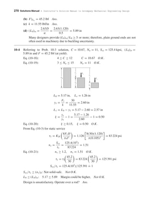
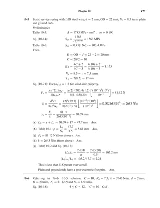
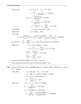
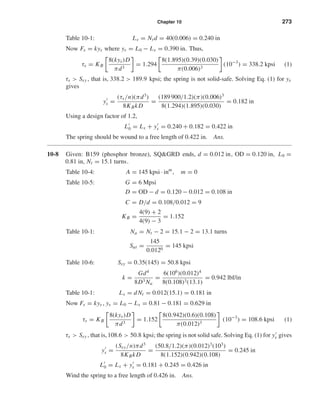
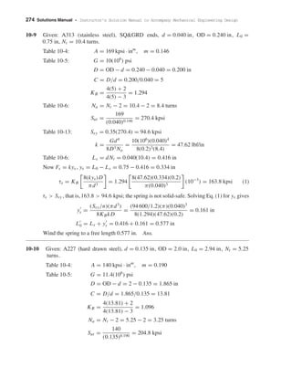
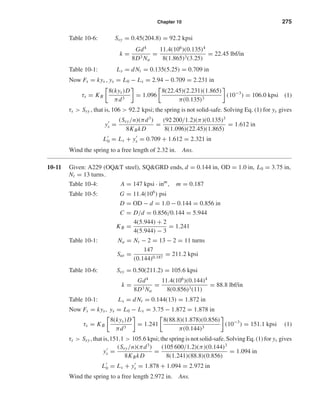
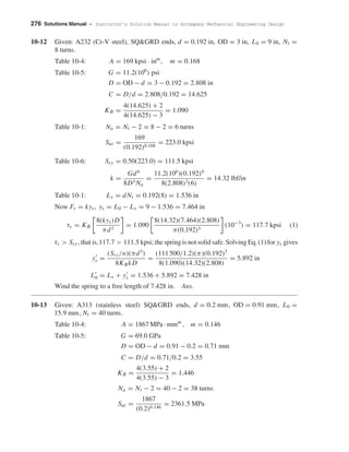
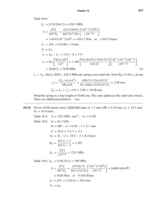
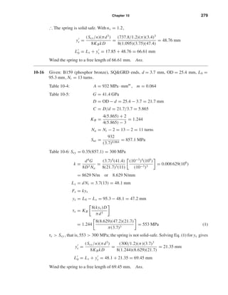
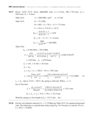
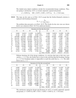
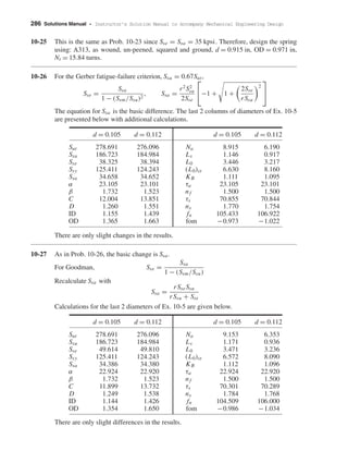
287. Chapter 10 287
10-28 Use: E = 28.6 Mpsi, G = 11.5 Mpsi, A = 140 kpsi · inm
, m = 0.190, rel cost = 1.
Try d = 0.067 in, Sut =
140
(0.067)0.190
= 234.0 kpsi
Table 10-6: Ssy = 0.45Sut = 105.3 kpsi
Table 10-7: Sy = 0.75Sut = 175.5 kpsi
Eq. (10-34) with D/d = C and C1 = C
σA =
Fmax
πd2
[(K)A(16C) + 4] =
Sy
ny
4C2
− C − 1
4C(C − 1)
(16C) + 4 =
πd2
Sy
ny Fmax
4C2
− C − 1 = (C − 1)
πd2
Sy
4ny Fmax
− 1
C2
−
1
4
1 +
πd2
Sy
4ny Fmax
− 1 C +
1
4
πd2
Sy
4ny Fmax
− 2 = 0
C =
1
2


πd2
Sy
16ny Fmax
±
πd2Sy
16ny Fmax
2
−
πd2Sy
4ny Fmax
+ 2


=
1
2
π(0.0672
)(175.5)(103
)
16(1.5)(18)
+
π(0.067)2(175.5)(103)
16(1.5)(18)
2
−
π(0.067)2(175.5)(103)
4(1.5)(18)
+ 2



= 4.590
D = Cd = 0.3075 in
Fi =
πd3
τi
8D
=
πd3
8D
33 500
exp(0.105C)
± 1000 4 −
C − 3
6.5
Use the lowest Fi in the preferred range. This results in the best fom.
Fi =
π(0.067)3
8(0.3075)
33 500
exp[0.105(4.590)]
− 1000 4 −
4.590 − 3
6.5
= 6.505 lbf
For simplicity, we will round up to the next integer or half integer;
therefore, use Fi = 7 lbf
k =
18 − 7
0.5
= 22 lbf/in
Na =
d4
G
8kD3
=
(0.067)4
(11.5)(106
)
8(22)(0.3075)3
= 45.28 turns
Nb = Na −
G
E
= 45.28 −
11.5
28.6
= 44.88 turns
L0 = (2C − 1 + Nb)d = [2(4.590) − 1 + 44.88](0.067) = 3.555 in
L18 lbf = 3.555 + 0.5 = 4.055 in
take positive root
shi20396_ch10.qxd 8/11/03 4:40 PM Page 287

288. Body: KB =
4C + 2
4C − 3
=
4(4.590) + 2
4(4.590) − 3
= 1.326
τmax =
8KB Fmax D
πd3
=
8(1.326)(18)(0.3075)
π(0.067)3
(10−3
) = 62.1 kpsi
(ny)body =
Ssy
τmax
=
105.3
62.1
= 1.70
r2 = 2d = 2(0.067) = 0.134 in, C2 =
2r2
d
=
2(0.134)
0.067
= 4
(K)B =
4C2 − 1
4C2 − 4
=
4(4) − 1
4(4) − 4
= 1.25
τB = (K)B
8Fmax D
πd3
= 1.25
8(18)(0.3075)
π(0.067)3
(10−3
) = 58.58 kpsi
(ny)B =
Ssy
τB
=
105.3
58.58
= 1.80
fom = −(1)
π2
d2
(Nb + 2)D
4
= −
π2
(0.067)2
(44.88 + 2)(0.3075)
4
= −0.160
Several diameters, evaluated using a spreadsheet, are shown below.
d: 0.067 0.072 0.076 0.081 0.085 0.09 0.095 0.104
Sut 233.977 230.799 228.441 225.692 223.634 221.219 218.958 215.224
Ssy 105.290 103.860 102.798 101.561 100.635 99.548 98.531 96.851
Sy 175.483 173.100 171.331 169.269 167.726 165.914 164.218 161.418
C 4.589 5.412 6.099 6.993 7.738 8.708 9.721 11.650
D 0.307 0.390 0.463 0.566 0.658 0.784 0.923 1.212
Fi (calc) 6.505 5.773 5.257 4.675 4.251 3.764 3.320 2.621
Fi (rd) 7.0 6.0 5.5 5.0 4.5 4.0 3.5 3.0
k 22.000 24.000 25.000 26.000 27.000 28.000 29.000 30.000
Na 45.29 27.20 19.27 13.10 9.77 7.00 5.13 3.15
Nb 44.89 26.80 18.86 12.69 9.36 6.59 4.72 2.75
L0 3.556 2.637 2.285 2.080 2.026 2.071 2.201 2.605
L18 lbf 4.056 3.137 2.785 2.580 2.526 2.571 2.701 3.105
KB 1.326 1.268 1.234 1.200 1.179 1.157 1.139 1.115
τmax 62.118 60.686 59.707 58.636 57.875 57.019 56.249 55.031
(ny)body 1.695 1.711 1.722 1.732 1.739 1.746 1.752 1.760
τB 58.576 59.820 60.495 61.067 61.367 61.598 61.712 61.712
(ny)B 1.797 1.736 1.699 1.663 1.640 1.616 1.597 1.569
(ny)A 1.500 1.500 1.500 1.500 1.500 1.500 1.500 1.500
fom −0.160 −0.144 −0.138 −0.135 −0.133 −0.135 −0.138 −0.154
Except for the 0.067 in wire, all springs satisfy the requirements of length and number of
coils. The 0.085 in wire has the highest fom.
288 Solutions Manual • Instructor’s Solution Manual to Accompany Mechanical Engineering Design
shi20396_ch10.qxd 8/11/03 4:40 PM Page 288

289. Chapter 10 289
10-29 Given: Nb = 84 coils, Fi = 16 lbf, OQ&T steel, OD = 1.5 in, d = 0.162 in.
D = 1.5 −0.162 =1.338 in
(a) Eq. (10-39):
L0 = 2(D − d) + (Nb + 1)d
= 2(1.338 − 0.162) + (84 + 1)(0.162) = 16.12 in Ans.
or 2d + L0 = 2(0.162) + 16.12 = 16.45 in overall.
(b) C =
D
d
=
1.338
0.162
= 8.26
KB =
4(8.26) + 2
4(8.26) − 3
= 1.166
τi = KB
8Fi D
πd3
= 1.166
8(16)(1.338)
π(0.162)3
= 14 950 psi Ans.
(c) From Table 10-5 use: G = 11.4(106
) psi and E = 28.5(106
) psi
Na = Nb +
G
E
= 84 +
11.4
28.5
= 84.4 turns
k =
d4
G
8D3 Na
=
(0.162)4
(11.4)(106
)
8(1.338)3(84.4)
= 4.855 lbf/in Ans.
(d) Table 10-4: A = 147 psi · inm
, m = 0.187
Sut =
147
(0.162)0.187
= 207.1 kpsi
Sy = 0.75(207.1) = 155.3 kpsi
Ssy = 0.50(207.1) = 103.5 kpsi
Body
F =
πd3
Ssy
π KB D
=
π(0.162)3
(103.5)(103
)
8(1.166)(1.338)
= 110.8 lbf
Torsional stress on hook point B
C2 =
2r2
d
=
2(0.25 + 0.162/2)
0.162
= 4.086
(K)B =
4C2 − 1
4C2 − 4
=
4(4.086) − 1
4(4.086) − 4
= 1.243
F =
π(0.162)3
(103.5)(103
)
8(1.243)(1.338)
= 103.9 lbf
Normal stress on hook point A
C1 =
2r1
d
=
1.338
0.162
= 8.26
(K)A =
4C2
1 − C1 − 1
4C1(C1 − 1)
=
4(8.26)2
− 8.26 − 1
4(8.26)(8.26 − 1)
= 1.099
shi20396_ch10.qxd 8/11/03 4:40 PM Page 289

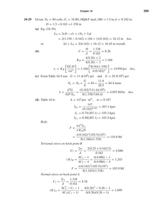
290. 290 Solutions Manual • Instructor’s Solution Manual to Accompany Mechanical Engineering Design
Syt = σ = F
16(K)A D
πd3
+
4
πd2
F =
155.3(103
)
[16(1.099)(1.338)]/[π(0.162)3] + {4/[π(0.162)2]}
= 85.8 lbf
= min(110.8, 103.9, 85.8) = 85.8 lbf Ans.
(e) Eq. (10-48):
y =
F − Fi
k
=
85.8 − 16
4.855
= 14.4 in Ans.
10-30 Fmin = 9 lbf, Fmax = 18 lbf
Fa =
18 − 9
2
= 4.5 lbf, Fm =
18 + 9
2
= 13.5 lbf
A313 stainless: 0.013 ≤ d ≤ 0.1 A = 169 kpsi · inm
, m = 0.146
0.1 ≤ d ≤ 0.2 A = 128 kpsi · inm
, m = 0.263
E = 28 Mpsi, G = 10 Gpsi
Try d = 0.081 in and refer to the discussion following Ex. 10-7
Sut =
169
(0.081)0.146
= 243.9 kpsi
Ssu = 0.67Sut = 163.4 kpsi
Ssy = 0.35Sut = 85.4 kpsi
Sy = 0.55Sut = 134.2 kpsi
Table 10-8: Sr = 0.45Sut = 109.8 kpsi
Se =
Sr /2
1 − [Sr /(2Sut)]2
=
109.8/2
1 − [(109.8/2)/243.9]2
= 57.8 kpsi
r = Fa/Fm = 4.5/13.5 = 0.333
Table 7-10: Sa =
r2
S2
ut
2Se

−1 + 1 +
2Se
rSut
2


Sa =
(0.333)2
(243.92
)
2(57.8)

−1 + 1 +
2(57.8)
0.333(243.9)
2

 = 42.2 kpsi
Hook bending
(σa)A = Fa (K)A
16C
πd2
+
4
πd2
=
Sa
(nf )A
=
Sa
2
4.5
πd2
(4C2
− C − 1)16C
4C(C − 1)
+ 4 =
Sa
2
This equation reduces to a quadratic in C—see Prob. 10-28
shi20396_ch10.qxd 8/11/03 4:40 PM Page 290

291. Chapter 10 291
The useable root for C is
C = 0.5

πd2
Sa
144
+
πd2Sa
144
2
−
πd2Sa
36
+ 2


= 0.5



π(0.081)2
(42.2)(103
)
144
+
π(0.081)2(42.2)(103)
144
2
−
π(0.081)2(42.2)(103)
36
+ 2



= 4.91
D = Cd = 0.398 in
Fi =
πd3
τi
8D
=
πd3
8D
33 500
exp(0.105C)
± 1000 4 −
C − 3
6.5
Use the lowest Fi in the preferred range.
Fi =
π(0.081)3
8(0.398)
33 500
exp[0.105(4.91)]
− 1000 4 −
4.91 − 3
6.5
= 8.55 lbf
For simplicity we will round up to next 1/4 integer.
Fi = 8.75 lbf
k =
18 − 9
0.25
= 36 lbf/in
Na =
d4
G
8kD3
=
(0.081)4
(10)(106
)
8(36)(0.398)3
= 23.7 turns
Nb = Na −
G
E
= 23.7 −
10
28
= 23.3 turns
L0 = (2C − 1 + Nb)d = [2(4.91) − 1 + 23.3](0.081) = 2.602 in
Lmax = L0 + (Fmax − Fi )/k = 2.602 + (18 − 8.75)/36 = 2.859 in
(σa)A =
4.5(4)
πd2
4C2
− C − 1
C − 1
+ 1
=
18(10−3
)
π(0.0812)
4(4.912
) − 4.91 − 1
4.91 − 1
+ 1 = 21.1 kpsi
(nf )A =
Sa
(σa)A
=
42.2
21.1
= 2 checks
Body: KB =
4C + 2
4C − 3
=
4(4.91) + 2
4(4.91) − 3
= 1.300
τa =
8(1.300)(4.5)(0.398)
π(0.081)3
(10−3
) = 11.16 kpsi
τm =
Fm
Fa
τa =
13.5
4.5
(11.16) = 33.47 kpsi
shi20396_ch10.qxd 8/11/03 4:40 PM Page 291

292. 292 Solutions Manual • Instructor’s Solution Manual to Accompany Mechanical Engineering Design
The repeating allowable stress from Table 7-8 is
Ssr = 0.30Sut = 0.30(243.9) = 73.17 kpsi
The Gerber intercept is
Sse =
73.17/2
1 − [(73.17/2)/163.4]2
= 38.5 kpsi
From Table 7-10,
(nf )body =
1
2
163.4
33.47
2
11.16
38.5



−1 + 1 +
2(33.47)(38.5)
163.4(11.16)
2



= 2.53
Let r2 = 2d = 2(0.081) = 0.162
C2 =
2r2
d
= 4, (K)B =
4(4) − 1
4(4) − 4
= 1.25
(τa)B =
(K)B
KB
τa =
1.25
1.30
(11.16) = 10.73 kpsi
(τm)B =
(K)B
KB
τm =
1.25
1.30
(33.47) = 32.18 kpsi
Table 10-8: (Ssr )B = 0.28Sut = 0.28(243.9) = 68.3 kpsi
(Sse)B =
68.3/2
1 − [(68.3/2)/163.4]2
= 35.7 kpsi
(nf )B =
1
2
163.4
32.18
2
10.73
35.7



−1 + 1 +
2(32.18)(35.7)
163.4(10.73)
2



= 2.51
Yield
Bending:
(σA)max =
4Fmax
πd2
(4C2
− C − 1)
C − 1
+ 1
=
4(18)
π(0.0812)
4(4.91)2
− 4.91 − 1
4.91 − 1
+ 1 (10−3
) = 84.4 kpsi
(ny)A =
134.2
84.4
= 1.59
Body:
τi = (Fi /Fa)τa = (8.75/4.5)(11.16) = 21.7 kpsi
r = τa/(τm − τi ) = 11.16/(33.47 − 21.7) = 0.948
(Ssa)y =
r
r + 1
(Ssy − τi ) =
0.948
0.948 + 1
(85.4 − 21.7) = 31.0 kpsi
(ny)body =
(Ssa)y
τa
=
31.0
11.16
= 2.78
Hook shear:
Ssy = 0.3Sut = 0.3(243.9) = 73.2 kpsi
τmax = (τa)B + (τm)B = 10.73 + 32.18 = 42.9 kpsi
shi20396_ch10.qxd 8/11/03 4:40 PM Page 292

293. Chapter 10 293
(ny)B =
73.2
42.9
= 1.71
fom = −
7.6π2
d2
(Nb + 2)D
4
= −
7.6π2
(0.081)2
(23.3 + 2)(0.398)
4
= −1.239
A tabulation of several wire sizes follow
d 0.081 0.085 0.092 0.098 0.105 0.12
Sut 243.920 242.210 239.427 237.229 234.851 230.317
Ssu 163.427 162.281 160.416 158.943 157.350 154.312
Sr 109.764 108.994 107.742 106.753 105.683 103.643
Se 57.809 57.403 56.744 56.223 55.659 54.585
Sa 42.136 41.841 41.360 40.980 40.570 39.786
C 4.903 5.484 6.547 7.510 8.693 11.451
D 0.397 0.466 0.602 0.736 0.913 1.374
OD 0.478 0.551 0.694 0.834 1.018 1.494
Fi (calc) 8.572 7.874 6.798 5.987 5.141 3.637
Fi (rd) 8.75 9.75 10.75 11.75 12.75 13.75
k 36.000 36.000 36.000 36.000 36.000 36.000
Na 23.86 17.90 11.38 8.03 5.55 2.77
Nb 23.50 17.54 11.02 7.68 5.19 2.42
L0 2.617 2.338 2.127 2.126 2.266 2.918
L18 lbf 2.874 2.567 2.328 2.300 2.412 3.036
(σa)A 21.068 20.920 20.680 20.490 20.285 19.893
(nf )A 2.000 2.000 2.000 2.000 2.000 2.000
KB 1.301 1.264 1.216 1.185 1.157 1.117
(τa)body 11.141 10.994 10.775 10.617 10.457 10.177
(τm)body 33.424 32.982 32.326 31.852 31.372 30.532
Ssr 73.176 72.663 71.828 71.169 70.455 69.095
Sse 38.519 38.249 37.809 37.462 37.087 36.371
(nf )body 2.531 2.547 2.569 2.583 2.596 2.616
(K)B 1.250 1.250 1.250 1.250 1.250 1.250
(τa)B 10.705 10.872 11.080 11.200 11.294 11.391
(τm)B 32.114 32.615 33.240 33.601 33.883 34.173
(Ssr )B 68.298 67.819 67.040 66.424 65.758 64.489
(Sse)B 35.708 35.458 35.050 34.728 34.380 33.717
(nf )B 2.519 2.463 2.388 2.341 2.298 2.235
Sy 134.156 133.215 131.685 130.476 129.168 126.674
(σA)max 84.273 83.682 82.720 81.961 81.139 79.573
(ny)A 1.592 1.592 1.592 1.592 1.592 1.592
τi 21.663 23.820 25.741 27.723 29.629 31.097
r 0.945 1.157 1.444 1.942 2.906 4.703
(Ssy)body 85.372 84.773 83.800 83.030 82.198 80.611
(Ssa)y 30.958 32.688 34.302 36.507 39.109 40.832
(ny)body 2.779 2.973 3.183 3.438 3.740 4.012
(Ssy)B 73.176 72.663 71.828 71.169 70.455 69.095
(τB)max 42.819 43.486 44.321 44.801 45.177 45.564
(ny)B 1.709 1.671 1.621 1.589 1.560 1.516
fom −1.246 −1.234 −1.245 −1.283 −1.357 −1.639
optimal fom
The shaded areas show the conditions not satisfied.
shi20396_ch10.qxd 8/11/03 4:40 PM Page 293

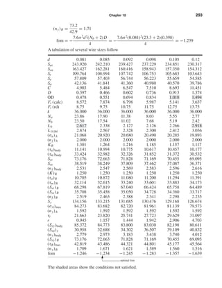
294. 294 Solutions Manual • Instructor’s Solution Manual to Accompany Mechanical Engineering Design
10-31 For the hook,
M = F R sin θ, ∂M/∂F = R sin θ
δF =
1
E I
π/2
0
F R2
sin2
R dθ =
π
2
P R3
E I
The total deflection of the body and the two hooks
δ =
8FD3
Nb
d4G
+ 2
π
2
F R3
E I
=
8FD3
Nb
d4G
+
π F(D/2)3
E(π/64)(d4)
=
8FD3
d4G
Nb +
G
E
=
8FD3
Na
d4G
І Na = Nb +
G
E
QED
10-32 Table 10-4 for A227:
A = 140 kpsi · inm
, m = 0.190
Table 10-5: E = 28.5(106
) psi
Sut =
140
(0.162)0.190
= 197.8 kpsi
Eq. (10-57):
Sy = σall = 0.78(197.8) = 154.3 kpsi
D = 1.25 − 0.162 = 1.088 in
C = D/d = 1.088/0.162 = 6.72
Ki =
4C2
− C − 1
4C(C − 1)
=
4(6.72)2
− 6.72 − 1
4(6.72)(6.72 − 1)
= 1.125
From σ = Ki
32M
πd3
Solving for M for the yield condition,
My =
πd3
Sy
32Ki
=
π(0.162)3
(154 300)
32(1.125)
= 57.2 lbf · in
Count the turns when M = 0
N = 2.5 −
My
d4 E/(10.8DN)
from which
N =
2.5
1 + [10.8DMy/(d4 E)]
=
2.5
1 + {[10.8(1.088)(57.2)]/[(0.162)4(28.5)(106)]}
= 2.417 turns
F
␪
R ϭ D͞2
shi20396_ch10.qxd 8/11/03 4:40 PM Page 294

295. Chapter 10 295
This means (2.5 − 2.417)(360◦
) or 29.9◦
from closed. Treating the hand force as in the
middle of the grip
r = 1 +
3.5
2
= 2.75 in
F =
My
r
=
57.2
2.75
= 20.8 lbf Ans.
10-33 The spring material and condition are unknown. Given d = 0.081 in and OD = 0.500,
(a) D = 0.500 − 0.081 = 0.419 in
Using E = 28.6 Mpsi for an estimate
k =
d4
E
10.8DN
=
(0.081)4
(28.6)(106
)
10.8(0.419)(11)
= 24.7 lbf · in/turn
for each spring. The moment corresponding to a force of 8 lbf
Fr = (8/2)(3.3125) = 13.25 lbf · in/spring
The fraction windup turn is
n =
Fr
k
=
13.25
24.7
= 0.536 turns
The arm swings through an arc of slightly less than 180◦
, say 165◦
. This uses up
165/360 or 0.458 turns. So n = 0.536 − 0.458 = 0.078 turns are left (or
0.078(360◦
) = 28.1◦
). The original configuration of the spring was
Ans.
(b)
C =
0.419
0.081
= 5.17
Ki =
4(5.17)2
− 5.17 − 1
4(5.17)(5.17 − 1)
= 1.168
σ = Ki
32M
πd3
= 1.168
32(13.25)
π(0.081)3
= 296 623 psi Ans.
To achieve this stress level, the spring had to have set removed.
10-34 Consider half and double results
Straight section: M = 3F R,
∂M
∂ P
= 3RF
3FR
L͞2
28.1Њ
shi20396_ch10.qxd 8/11/03 4:40 PM Page 295

296. 296 Solutions Manual • Instructor’s Solution Manual to Accompany Mechanical Engineering Design
Upper 180◦
section:
M = F[R + R(1 − cos φ)]
= F R(2 − cos φ),
∂M
∂ P
= R(2 − cos φ)
Lower section: M = F R sin θ
∂M
∂ P
= R sin θ
Considering bending only:
δ =
2
E I
L/2
0
9F R2
dx +
π
0
F R2
(2 − cos φ)2
R dφ +
π/2
0
F(R sin θ)2
R dθ
=
2F
E I
9
2
R2
L + R3
4π − 4 sin φ
π
0
+
π
2
+ R3 π
4
=
2F R2
E I
19π
4
R +
9
2
L =
F R2
2E I
(19π R + 18L) Ans.
10-35 Computer programs will vary.
10-36 Computer programs will vary.
␾
␪
F
R
shi20396_ch10.qxd 8/11/03 4:40 PM Page 296

297. Chapter 11
11-1 For the deep-groove 02-series ball bearing with R = 0.90, the design life xD, in multiples
of rating life, is
xD =
30 000(300)(60)
106
= 540 Ans.
The design radial load FD is
FD = 1.2(1.898) = 2.278 kN
From Eq. (11-6),
C10 = 2.278
540
0.02 + 4.439[ln(1/0.9)]1/1.483
1/3
= 18.59 kN Ans.
Table 11-2: Choose a 02-30 mm with C10 = 19.5 kN. Ans.
Eq. (11-18):
R = exp −
540(2.278/19.5)3
− 0.02
4.439
1.483
= 0.919 Ans.
11-2 For the Angular-contact 02-series ball bearing as described, the rating life multiple is
xD =
50 000(480)(60)
106
= 1440
The design load is radial and equal to
FD = 1.4(610) = 854 lbf = 3.80 kN
Eq. (11-6):
C10 = 854
1440
0.02 + 4.439[ln(1/0.9)]1/1.483
1/3
= 9665 lbf = 43.0 kN
Table 11-2: Select a 02-55 mm with C10 = 46.2 kN. Ans.
Using Eq. (11-18),
R = exp −
1440(3.8/46.2)3
− 0.02
4.439
1.483
= 0.927 Ans.
shi20396_ch11.qxd 8/12/03 9:51 AM Page 297

298. 298 Solutions Manual • Instructor’s Solution Manual to Accompany Mechanical Engineering Design
11-3 For the straight-Roller 03-series bearing selection, xD = 1440 rating lives from Prob. 11-2
solution.
FD = 1.4(1650) = 2310 lbf = 10.279 kN
C10 = 10.279
1440
1
3/10
= 91.1 kN
Table 11-3: Select a 03-55 mm with C10 = 102 kN. Ans.
Using Eq. (11-18),
R = exp −
1440(10.28/102)10/3
− 0.02
4.439
1.483
= 0.942 Ans.
11-4 We can choose a reliability goal of
√
0.90 = 0.95 for each bearing. We make the selec-
tions, find the existing reliabilities, multiply them together, and observe that the reliability
goal is exceeded due to the roundup of capacity upon table entry.
Another possibility is to use the reliability of one bearing, say R1. Then set the relia-
bility goal of the second as
R2 =
0.90
R1
or vice versa. This gives three pairs of selections to compare in terms of cost, geometry im-
plications, etc.
11-5 Establish a reliability goal of
√
0.90 = 0.95 for each bearing. For a 02-series angular con-
tact ball bearing,
C10 = 854
1440
0.02 + 4.439[ln(1/0.95)]1/1.483
1/3
= 11 315 lbf = 50.4 kN
Select a 02-60 mm angular-contact bearing with C10 = 55.9 kN.
RA = exp −
1440(3.8/55.9)3
− 0.02
4.439
1.483
= 0.969
For a 03-series straight-roller bearing,
C10 = 10.279
1440
0.02 + 4.439[ln(1/0.95)]1/1.483
3/10
= 105.2 kN
Select a 03-60 mm straight-roller bearing with C10 = 123 kN.
RB = exp −
1440(10.28/123)10/3
− 0.02
4.439
1.483
= 0.977
shi20396_ch11.qxd 8/12/03 9:51 AM Page 298

299. Chapter 11 299
Form a table of existing reliabilities
Rgoal RA RB 0.912
0.90 0.927 0.941 0.872
0.95 0.969 0.977 0.947
0.906
The possible products in the body of the table are displayed to the right of the table. One,
0.872, is predictably less than the overall reliability goal. The remaining three are the
choices for a combined reliability goal of 0.90. Choices can be compared for the cost of
bearings, outside diameter considerations, bore implications for shaft modifications and
housing modifications.
The point is that the designer has choices. Discover them before making the selection
decision. Did the answer to Prob. 11-4 uncover the possibilities?
To reduce the work to fill in the body of the table above, a computer program can be
helpful.
11-6 Choose a 02-series ball bearing from manufacturer #2, having a service factor of 1. For
Fr = 8 kN and Fa = 4 kN
xD =
5000(900)(60)
106
= 270
Eq. (11-5):
C10 = 8
270
0.02 + 4.439[ln(1/0.90)]1/1.483
1/3
= 51.8 kN
Trial #1: From Table (11-2) make a tentative selection of a deep-groove 02-70 mm with
C0 = 37.5 kN.
Fa
C0
=
4
37.5
= 0.107
Table 11-1:
Fa/(V Fr ) = 0.5 > e
X2 = 0.56, Y2 = 1.46
Eq. (11-9):
Fe = 0.56(1)(8) + 1.46(4) = 10.32 kN
Eq. (11-6):
C10 = 10.32
270
1
1/3
= 66.7 kN > 61.8 kN
Trial #2: From Table 11-2 choose a 02-80 mm having C10 = 70.2 and C0 = 45.0.
Check:
Fa
C0
=
4
45
= 0.089
shi20396_ch11.qxd 8/12/03 9:51 AM Page 299

300. 300 Solutions Manual • Instructor’s Solution Manual to Accompany Mechanical Engineering Design
Table 11-1: X2 = 0.56, Y2 = 1.53
Fe = 0.56(8) + 1.53(4) = 10.60 kN
Eq. (11-6):
C10 = 10.60
270
1
1/3
= 68.51 kN < 70.2 kN
∴ Selection stands.
Decision: Specify a 02-80 mm deep-groove ball bearing. Ans.
11-7 From Prob. 11-6, xD = 270 and the final value of Fe is 10.60 kN.
C10 = 10.6
270
0.02 + 4.439[ln(1/0.96)]1/1.483
1/3
= 84.47 kN
Table 11-2: Choose a deep-groove ball bearing, based upon C10 load ratings.
Trial #1:
Tentatively select a 02-90 mm.
C10 = 95.6, C0 = 62 kN
Fa
C0
=
4
62
= 0.0645
From Table 11-1, interpolate for Y2.
Fa/C0 Y2
0.056 1.71
0.0645 Y2
0.070 1.63
Y2 − 1.71
1.63 − 1.71
=
0.0645 − 0.056
0.070 − 0.056
= 0.607
Y2 = 1.71 + 0.607(1.63 − 1.71) = 1.661
Fe = 0.56(8) + 1.661(4) = 11.12 kN
C10 = 11.12
270
0.02 + 4.439[ln(1/0.96)]1/1.483
1/3
= 88.61 kN < 95.6 kN
Bearing is OK.
Decision: Specify a deep-groove 02-90 mm ball bearing. Ans.
shi20396_ch11.qxd 8/12/03 9:51 AM Page 300

301. Chapter 11 301
11-8 For the straight cylindrical roller bearing specified with a service factor of 1, R = 0.90 and
Fr = 12 kN
xD =
4000(750)(60)
106
= 180
C10 = 12
180
1
3/10
= 57.0 kN Ans.
11-9
Assume concentrated forces as shown.
Pz = 8(24) = 192 lbf
Py = 8(30) = 240 lbf
T = 192(2) = 384 lbf · in
T x
= −384 + 1.5F cos 20◦
= 0
F =
384
1.5(0.940)
= 272 lbf
Mz
O = 5.75Py + 11.5R
y
A − 14.25F sin 20◦
= 0;
thus 5.75(240) + 11.5R
y
A − 14.25(272)(0.342) = 0
R
y
A = −4.73 lbf
M
y
O = −5.75Pz − 11.5Rz
A − 14.25F cos 20◦
= 0;
thus −5.75(192) − 11.5Rz
A − 14.25(272)(0.940) = 0
Rz
A = −413 lbf; RA = [(−413)2
+ (−4.73)2
]1/2
= 413 lbf
Fz
= Rz
O + Pz + Rz
A + F cos 20◦
= 0
Rz
O + 192 − 413 + 272(0.940) = 0
Rz
O = −34.7 lbf
B
O
z
11
1
2
"
Rz
O
Ry
O
Pz
Py
T
F
20Њ
R
y
A
R
z
A
A
T
y
2
3
4
"
x
shi20396_ch11.qxd 8/12/03 9:51 AM Page 301

302. 302 Solutions Manual • Instructor’s Solution Manual to Accompany Mechanical Engineering Design
Fy
= R
y
O + Py + R
y
A − F sin 20◦
= 0
R
y
O + 240 − 4.73 − 272(0.342) = 0
R
y
O = −142 lbf
RO = [(−34.6)2
+ (−142)2
]1/2
= 146 lbf
So the reaction at A governs.
Reliability Goal:
√
0.92 = 0.96
FD = 1.2(413) = 496 lbf
xD = 30 000(300)(60/106
) = 540
C10 = 496
540
0.02 + 4.439[ln(1/0.96)]1/1.483
1/3
= 4980 lbf = 22.16 kN
A 02-35 bearing will do.
Decision: Specify an angular-contact 02-35 mm ball bearing for the locations at A and O.
Check combined reliability. Ans.
11-10 For a combined reliability goal of 0.90, use
√
0.90 = 0.95 for the individual bearings.
x0 =
50 000(480)(60)
106
= 1440
The resultant of the given forces are RO = 607 lbf and RB = 1646 lbf.
At O: Fe = 1.4(607) = 850 lbf
Ball: C10 = 850
1440
0.02 + 4.439[ln(1/0.95)]1/1.483
1/3
= 11 262 lbf or 50.1 kN
Select a 02-60 mm angular-contact ball bearing with a basic load rating of 55.9 kN.
At B: Fe = 1.4(1646) = 2304 lbf
Roller: C10 = 2304
1440
0.02 + 4.439[ln(1/0.95)]1/1.483
3/10
= 23 576 lbf or 104.9 kN
Select a 02-80 mm cylindrical roller or a 03-60 mm cylindrical roller. The 03-series roller
has the same bore as the 02-series ball.
z
20
16
10
O
FA
RO
RB
B
A
C
y
x
FC
20Њ
shi20396_ch11.qxd 8/12/03 9:51 AM Page 302

303. Chapter 11 303
11-11 The reliability of the individual bearings is R =
√
0.999 = 0.9995
From statics,
R
y
O = −163.4 N, Rz
O = 107 N, RO = 195 N
R
y
E = −89.1 N, Rz
E = −174.4 N, RE = 196 N
xD =
60 000(1200)(60)
106
= 4320
C10 = 0.196
4340
0.02 + 4.439[ln(1/0.9995)]1/1.483
1/3
= 8.9 kN
A 02-25 mm deep-groove ball bearing has a basic load rating of 14.0 kN which is ample.
An extra-light bearing could also be investigated.
11-12 Given:
Fr A = 560 lbf or 2.492 kN
Fr B = 1095 lbf or 4.873 kN
Trial #1: Use KA = KB = 1.5 and from Table 11-6 choose an indirect mounting.
0.47Fr A
KA
<? >
0.47Fr B
KB
− (−1)(0)
0.47(2.492)
1.5
<? >
0.47(4.873)
1.5
0.781 < 1.527 Therefore use the upper line of Table 11-6.
FaA = FaB =
0.47Fr B
KB
= 1.527 kN
PA = 0.4Fr A + KA FaA = 0.4(2.492) + 1.5(1.527) = 3.29 kN
PB = Fr B = 4.873 kN
150
300
400
A
O
Fz
A
F
y
A
E
Rz
E
R
y
E
FC
C
Rz
O
R
y
O
z
x
y
shi20396_ch11.qxd 8/12/03 9:51 AM Page 303

304. 304 Solutions Manual • Instructor’s Solution Manual to Accompany Mechanical Engineering Design
Fig. 11-16: fT = 0.8
Fig. 11-17: fV = 1.07
Thus, a3l = fT fV = 0.8(1.07) = 0.856
Individual reliability: Ri =
√
0.9 = 0.95
Eq. (11-17):
(C10)A = 1.4(3.29)
40 000(400)(60)
4.48(0.856)(1 − 0.95)2/3(90)(106)
0.3
= 11.40 kN
(C10)B = 1.4(4.873)
40 000(400)(60)
4.48(0.856)(1 − 0.95)2/3(90)(106)
0.3
= 16.88 kN
From Fig. 11-14, choose cone 32305 and cup 32305 which provide Fr = 17.4 kN and
K = 1.95. With K = 1.95 for both bearings, a second trial validates the choice of cone
32305 and cup 32305. Ans.
11-13
R =
√
0.95 = 0.975
T = 240(12)(cos 20◦
) = 2706 lbf · in
F =
2706
6 cos 25◦
= 498 lbf
In xy-plane:
MO = −82.1(16) − 210(30) + 42R
y
C = 0
R
y
C = 181 lbf
R
y
O = 82 + 210 − 181 = 111 lbf
In xz-plane:
MO = 226(16) − 452(30) − 42Rz
c = 0
Rz
C = −237 lbf
Rz
O = 226 − 451 + 237 = 12 lbf
RO = (1112
+ 122
)1/2
= 112 lbf Ans.
RC = (1812
+ 2372
)1/2
= 298 lbf Ans.
FeO = 1.2(112) = 134.4 lbf
FeC = 1.2(298) = 357.6 lbf
xD =
40 000(200)(60)
106
= 480
z
14"
16"
12"
Rz
O
R
z
C
R
y
O
A
B
C
R
y
C
O
451
210
226
T
T
82.1
x
y
shi20396_ch11.qxd 8/12/03 9:51 AM Page 304

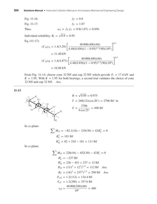
305. Chapter 11 305
(C10)O = 134.4
480
0.02 + 4.439[ln(1/0.975)]1/1.483
1/3
= 1438 lbf or 6.398 kN
(C10)C = 357.6
480
0.02 + 4.439[ln(1/0.975)]1/1.483
1/3
= 3825 lbf or 17.02 kN
Bearing at O: Choose a deep-groove 02-12 mm. Ans.
Bearing at C: Choose a deep-groove 02-30 mm. Ans.
There may be an advantage to the identical 02-30 mm bearings in a gear-reduction unit.
11-14 Shafts subjected to thrust can be constrained by bearings, one of which supports the thrust.
The shaft floats within the endplay of the second (Roller) bearing. Since the thrust force
here is larger than any radial load, the bearing absorbing the thrust is heavily loaded com-
pared to the other bearing. The second bearing is thus oversized and does not contribute
measurably to the chance of failure. This is predictable. The reliability goal is not
√
0.99,
but 0.99 for the ball bearing. The reliability of the roller is 1. Beginning here saves effort.
Bearing at A (Ball)
Fr = (362
+ 2122
)1/2
= 215 lbf = 0.957 kN
Fa = 555 lbf = 2.47 kN
Trial #1:
Tentatively select a 02-85 mm angular-contact with C10 = 90.4 kN and C0 = 63.0 kN.
Fa
C0
=
2.47
63.0
= 0.0392
xD =
25 000(600)(60)
106
= 900
Table 11-1: X2 = 0.56, Y2 = 1.88
Fe = 0.56(0.957) + 1.88(2.47) = 5.18 kN
FD = fA Fe = 1.3(5.18) = 6.73 kN
C10 = 6.73
900
0.02 + 4.439[ln(1/0.99)]1/1.483
1/3
= 107.7 kN > 90.4 kN
Trial #2:
Tentatively select a 02-95 mm angular-contact ball with C10 = 121 kN and C0 = 85 kN.
Fa
C0
=
2.47
85
= 0.029
shi20396_ch11.qxd 8/12/03 9:51 AM Page 305

306. 306 Solutions Manual • Instructor’s Solution Manual to Accompany Mechanical Engineering Design
Table 11-1: Y2 = 1.98
Fe = 0.56(0.957) + 1.98(2.47) = 5.43 kN
FD = 1.3(5.43) = 7.05 kN
C10 = 7.05
900
0.02 + 4.439[ln(1/0.99)]1/1.483
1/3
= 113 kN < 121 kN O.K.
Select a 02-95 mm angular-contact ball bearing. Ans.
Bearing at B (Roller): Any bearing will do since R = 1. Let’s prove it. From Eq. (11-18)
when
af FD
C10
3
xD < x0 R = 1
The smallest 02-series roller has a C10 = 16.8 kN for a basic load rating.
0.427
16.8
3
(900) < ? > 0.02
0.0148 < 0.02 ∴ R = 1
Spotting this early avoided rework from
√
0.99 = 0.995.
Any 02-series roller bearing will do. Same bore or outside diameter is a common choice.
(Why?) Ans.
11-15 Hoover Ball-bearing Division uses the same 2-parameter Weibull model as Timken:
b = 1.5, θ = 4.48. We have some data. Let’s estimate parameters b and θ from it. In
Fig. 11-5, we will use line AB. In this case, B is to the right of A.
For F = 18 kN, (x)1 =
115(2000)(16)
106
= 13.8
This establishes point 1 on the R = 0.90 line.
1
0
10
2
10
18
1 2
39.6
100
1
10
13.8 72
1
100 x
2 log x
F
A B
log F
R ϭ 0.90
R ϭ 0.20
shi20396_ch11.qxd 8/12/03 9:51 AM Page 306

307. Chapter 11 307
The R = 0.20 locus is above and parallel to the R = 0.90 locus. For the two-parameter
Weibull distribution, x0 = 0 and points A and B are related by:
xA = θ[ln(1/0.90)]1/b
(1)
xB = θ[ln(1/0.20)]1/b
and xB/xA is in the same ratio as 600/115. Eliminating θ
b =
ln[ln(1/0.20)/ ln(1/0.90)]
ln(600/115)
= 1.65
Solving for θ in Eq. (1)
θ =
xA
[ln(1/RA)]1/1.65
=
1
[ln(1/0.90)]1/1.65
= 3.91
Therefore, for the data at hand,
R = exp −
x
3.91
1.65
Check R at point B: xB = (600/115) = 5.217
R = exp −
5.217
3.91
1.65
= 0.20
Note also, for point 2 on the R = 0.20 line.
log(5.217) − log(1) = log(xm)2 − log(13.8)
(xm)2 = 72
11-16 This problem is rich in useful variations. Here is one.
Decision: Make straight roller bearings identical on a given shaft. Use a reliability goal of
(0.99)1/6
= 0.9983.
Shaft a
Fr
A = (2392
+ 1112
)1/2
= 264 lbf or 1.175 kN
Fr
B = (5022
+ 10752
)1/2
= 1186 lbf or 5.28 kN
Thus the bearing at B controls
xD =
10 000(1200)(60)
106
= 720
0.02 + 4.439[ln(1/0.9983)]1/1.483
= 0.080 26
C10 = 1.2(5.2)
720
0.080 26
0.3
= 97.2 kN
Select either a 02-80 mm with C10 = 106 kN or a 03-55 mm with C10 = 102 kN
shi20396_ch11.qxd 8/12/03 9:51 AM Page 307

308. 308 Solutions Manual • Instructor’s Solution Manual to Accompany Mechanical Engineering Design
Shaft b
Fr
C = (8742
+ 22742
)1/2
= 2436 lbf or 10.84 kN
Fr
D = (3932
+ 6572
)1/2
= 766 lbf or 3.41 kN
The bearing at C controls
xD =
10 000(240)(60)
106
= 144
C10 = 1.2(10.84)
144
0.0826
0.3
= 122 kN
Select either a 02-90 mm with C10 = 142 kN or a 03-60 mm with C10 = 123 kN
Shaft c
Fr
E = (11132
+ 23852
)1/2
= 2632 lbf or 11.71 kN
Fr
F = (4172
+ 8952
)1/2
= 987 lbf or 4.39 kN
The bearing at E controls
xD = 10 000(80)(60/106
) = 48
C10 = 1.2(11.71)
48
0.0826
0.3
= 94.8 kN
Select a 02-80 mm with C10 = 106 kN or a 03-60 mm with C10 = 123 kN
11-17 The horizontal separation of the R = 0.90 loci in a log F-log x plot such as Fig. 11-5
will be demonstrated. We refer to the solution of Prob. 11-15 to plot point G (F =
18 kN, xG = 13.8). We know that (C10)1 = 39.6 kN, x1 = 1. This establishes the unim-
proved steel R = 0.90 locus, line AG. For the improved steel
(xm)1 =
360(2000)(60)
106
= 43.2
We plot point G (F = 18 kN, xG = 43.2), and draw the R = 0.90 locus AmG parallel
to AG
1
0
10
2
10
18
G GЈ
39.6
55.8
100
1
10
13.8
1
100
2
x
log x
F
A
Am
Improved steel
log F
Unimproved steel
43.2
R ϭ 0.90
R ϭ 0.90
1
3
1
3
shi20396_ch11.qxd 8/12/03 9:51 AM Page 308

309. Chapter 11 309
We can calculate (C10)m by similar triangles.
log(C10)m − log 18
log 43.2 − log 1
=
log 39.6 − log 18
log 13.8 − log 1
log(C10)m =
log 43.2
log 13.8
log
39.6
18
+ log 18
(C10)m = 55.8 kN
The usefulness of this plot is evident. The improvement is 43.2/13.8 = 3.13 fold in life.
This result is also available by (L10)m/(L10)1 as 360/115 or 3.13 fold, but the plot shows
the improvement is for all loading. Thus, the manufacturer’s assertion that there is at least
a 3-fold increase in life has been demonstrated by the sample data given. Ans.
11-18 Express Eq. (11-1) as
Fa
1 L1 = Ca
10L10 = K
For a ball bearing, a = 3 and for a 02-30 mm angular contact bearing, C10 = 20.3 kN.
K = (20.3)3
(106
) = 8.365(109
)
At a load of 18 kN, life L1 is given by:
L1 =
K
Fa
1
=
8.365(109
)
183
= 1.434(106
) rev
For a load of 30 kN, life L2 is:
L2 =
8.365(109
)
303
= 0.310(106
) rev
In this case, Eq. (7-57) – the Palmgren-Miner cycle ratio summation rule – can be ex-
pressed as
l1
L1
+
l2
L2
= 1
Substituting,
200 000
1.434(106)
+
l2
0.310(106)
= 1
l2 = 0.267(106
) rev Ans.
Check:
200 000
1.434(106)
+
0.267(106
)
0.310(106)
= 1 O.K.
11-19 Total life in revolutions
Let:
l = total turns
f1 = fraction of turns at F1
f2 = fraction of turns at F2
shi20396_ch11.qxd 8/12/03 9:51 AM Page 309

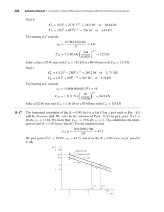
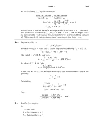
310. 310 Solutions Manual • Instructor’s Solution Manual to Accompany Mechanical Engineering Design
From the solution of Prob. 11-18, L1 = 1.434(106
) rev and L2 = 0.310(106
) rev.
Palmgren-Miner rule:
l1
L1
+
l2
L2
=
f1l
L1
+
f2l
L2
= 1
from which
l =
1
f1/L1 + f2/L2
l =
1
{0.40/[1.434(106)]} + {0.60/[0.310(106)]}
= 451 585 rev Ans.
Total life in loading cycles
4 min at 2000 rev/min = 8000 rev
6 min
10 min/cycle
at 2000 rev/min =
12 000 rev
20 000 rev/cycle
451 585 rev
20 000 rev/cycle
= 22.58 cycles Ans.
Total life in hours
10
min
cycle
22.58 cycles
60 min/h
= 3.76 h Ans.
11-20 While we made some use of the log F-log x plot in Probs. 11-15 and 11-17, the principal
use of Fig. 11-5 is to understand equations (11-6) and (11-7) in the discovery of the cata-
log basic load rating for a case at hand.
Point D
FD = 495.6 lbf
log FD = log 495.6 = 2.70
xD =
30 000(300)(60)
106
= 540
log xD = log 540 = 2.73
KD = F3
DxD = (495.6)3
(540)
= 65.7(109
) lbf3
· turns
log KD = log[65.7(109
)] = 10.82
FD has the following uses: Fdesign, Fdesired, Fe when a thrust load is present. It can include
application factor af , or not. It depends on context.
shi20396_ch11.qxd 8/12/03 9:51 AM Page 310

311. Chapter 11 311
Point B
xB = 0.02 + 4.439[ln(1/0.99)]1/1.483
= 0.220 turns
log xB = log 0.220 = −0.658
FB = FD
xD
xB
1/3
= 495.6
540
0.220
1/3
= 6685 lbf
Note: Example 11-3 used Eq. (11-7). Whereas, here we basically used Eq. (11-6).
log FB = log(6685) = 3.825
KD = 66853
(0.220) = 65.7(109
) lbf3
· turns (as it should)
Point A
FA = FB = C10 = 6685 lbf
log C10 = log(6685) = 3.825
xA = 1
log xA = log(1) = 0
K10 = F3
AxA = C3
10(1) = 66853
= 299(109
) lbf3
· turns
Note that KD/K10 = 65.7(109
)/[299(109
)] = 0.220, which is xB. This is worth knowing
since
K10 =
KD
xB
log K10 = log[299(109
)] = 11.48
Now C10 = 6685 lbf = 29.748 kN, which is required for a reliability goal of 0.99. If we
select an angular contact 02-40 mm ball bearing, then C10 = 31.9 kN = 7169 lbf.
0.1
Ϫ1
Ϫ0.658
1
0
10
1
102
2
102
2
103
495.6
6685
3
104
4
103
3
x
log x
F
A
D
B
log F
540
shi20396_ch11.qxd 8/12/03 9:51 AM Page 311

312. Chapter 12
12-1 Given dmax = 1.000 in and bmin = 1.0015 in, the minimum radial clearance is
cmin =
bmin − dmax
2
=
1.0015 − 1.000
2
= 0.000 75 in
Also l/d = 1
r ˙= 1.000/2 = 0.500
r/c = 0.500/0.000 75 = 667
N = 1100/60 = 18.33 rev/s
P = W/(ld) = 250/[(1)(1)] = 250 psi
Eq. (12-7): S = (6672
)
8(10−6
)(18.33)
250
= 0.261
Fig. 12-16: h0/c = 0.595
Fig. 12-19: Q/(rcNl) = 3.98
Fig. 12-18: f r/c = 5.8
Fig. 12-20: Qs/Q = 0.5
h0 = 0.595(0.000 75) = 0.000 466 in Ans.
f =
5.8
r/c
=
5.8
667
= 0.0087
The power loss in Btu/s is
H =
2π f Wr N
778(12)
=
2π(0.0087)(250)(0.5)(18.33)
778(12)
= 0.0134 Btu/s Ans.
Q = 3.98rcNl = 3.98(0.5)(0.000 75)(18.33)(1) = 0.0274 in3
/s
Qs = 0.5(0.0274) = 0.0137 in3
/s Ans.
12-2
cmin =
bmin − dmax
2
=
1.252 − 1.250
2
= 0.001 in
r
.
= 1.25/2 = 0.625 in
r/c = 0.625/0.001 = 625
N = 1150/60 = 19.167 rev/s
P =
400
1.25(2.5)
= 128 psi
l/d = 2.5/1.25 = 2
S =
(6252
)(10)(10−6
)(19.167)
128
= 0.585
shi20396_ch12.qxd 8/29/03 2:21 PM Page 312

313. Chapter 12 313
The interpolation formula of Eq. (12-16) will have to be used. From Figs. 12-16, 12-21,
and 12-19
For l/d = ∞, ho/c = 0.96, P/pmax = 0.84,
Q
rcNl
= 3.09
l/d = 1, ho/c = 0.77, P/pmax = 0.52,
Q
rcNl
= 3.6
l/d =
1
2
, ho/c = 0.54, P/pmax = 0.42,
Q
rcNl
= 4.4
l/d =
1
4
, ho/c = 0.31, P/pmax = 0.28,
Q
rcNl
= 5.25
Equation (12-16) is easily programmed by code or by using a spreadsheet. The results are:
l/d y∞ y1 y1/2 y1/4 yl/d
ho/c 2 0.96 0.77 0.54 0.31 0.88
P/pmax 2 0.84 0.52 0.42 0.28 0.64
Q/rcNl 2 3.09 3.60 4.40 5.25 3.28
∴ ho = 0.88(0.001) = 0.000 88 in Ans.
pmax =
128
0.64
= 200 psi Ans.
Q = 3.28(0.625)(0.001)(19.167)(2.5) = 0.098 in3
/s Ans.
12-3
cmin =
bmin − dmax
2
=
3.005 − 3.000
2
= 0.0025 in
r
.
= 3.000/2 = 1.500 in
l/d = 1.5/3 = 0.5
r/c = 1.5/0.0025 = 600
N = 600/60 = 10 rev/s
P =
800
1.5(3)
= 177.78 psi
Fig. 12-12: SAE 10, µ = 1.75 µreyn
S = (6002
)
1.75(10−6
)(10)
177.78
= 0.0354
Figs. 12-16 and 12-21: ho/c = 0.11, P/pmax = 0.21
ho = 0.11(0.0025) = 0.000 275 in Ans.
pmax = 177.78/0.21 = 847 psi Ans.
shi20396_ch12.qxd 8/29/03 2:21 PM Page 313

314. 314 Solutions Manual • Instructor’s Solution Manual to Accompany Mechanical Engineering Design
Fig. 12-12: SAE 40, µ = 4.5 µreyn
S = 0.0354
4.5
1.75
= 0.0910
ho/c = 0.19, P/pmax = 0.275
ho = 0.19(0.0025) = 0.000 475 in Ans.
pmax = 177.78/0.275 = 646 psi Ans.
12-4
cmin =
bmin − dmax
2
=
3.006 − 3.000
2
= 0.003
r
.
= 3.000/2 = 1.5 in
l/d = 1
r/c = 1.5/0.003 = 500
N = 750/60 = 12.5 rev/s
P =
600
3(3)
= 66.7 psi
Fig. 12-14: SAE 10W, µ = 2.1 µreyn
S = (5002
)
2.1(10−6
)(12.5)
66.7
= 0.0984
From Figs. 12-16 and 12-21:
ho/c = 0.34, P/pmax = 0.395
ho = 0.34(0.003) = 0.001 020 in Ans.
pmax =
66.7
0.395
= 169 psi Ans.
Fig. 12-14: SAE 20W-40, µ = 5.05 µreyn
S = (5002
)
5.05(10−6
)(12.5)
66.7
= 0.237
From Figs. 12-16 and 12-21:
ho/c = 0.57, P/pmax = 0.47
ho = 0.57(0.003) = 0.001 71 in Ans.
pmax =
66.7
0.47
= 142 psi Ans.
shi20396_ch12.qxd 8/29/03 2:21 PM Page 314

315. Chapter 12 315
12-5
cmin =
bmin − dmax
2
=
2.0024 − 2
2
= 0.0012 in
r
.
=
d
2
=
2
2
= 1 in, l/d = 1/2 = 0.50
r/c = 1/0.0012 = 833
N = 800/60 = 13.33 rev/s
P =
600
2(1)
= 300 psi
Fig. 12-12: SAE 20, µ = 3.75 µreyn
S = (8332
)
3.75(10−6
)(13.3)
300
= 0.115
From Figs. 12-16, 12-18 and 12-19:
ho/c = 0.23, r f/c = 3.8, Q/(rcNl) = 5.3
ho = 0.23(0.0012) = 0.000 276 in Ans.
f =
3.8
833
= 0.004 56
The power loss due to friction is
H =
2π f Wr N
778(12)
=
2π(0.004 56)(600)(1)(13.33)
778(12)
= 0.0245 Btu/s Ans.
Q = 5.3rcNl
= 5.3(1)(0.0012)(13.33)(1)
= 0.0848 in3
/s Ans.
12-6
cmin =
bmin − dmax
2
=
25.04 − 25
2
= 0.02 mm
r ˙= d/2 = 25/2 = 12.5 mm, l/d = 1
r/c = 12.5/0.02 = 625
N = 1200/60 = 20 rev/s
P =
1250
252
= 2 MPa
For µ = 50 MPa · s, S = (6252
)
50(10−3
)(20)
2(106)
= 0.195
From Figs. 12-16, 12-18 and 12-20:
ho/c = 0.52, f r/c = 4.5, Qs/Q = 0.57
ho = 0.52(0.02) = 0.0104 mm Ans.
f =
4.5
625
= 0.0072
T = f Wr = 0.0072(1.25)(12.5) = 0.1125 N · m
shi20396_ch12.qxd 8/29/03 2:21 PM Page 315

316. 316 Solutions Manual • Instructor’s Solution Manual to Accompany Mechanical Engineering Design
The power loss due to friction is
H = 2πT N = 2π(0.1125)(20) = 14.14 W Ans.
Qs = 0.57Q The side flow is 57% of Q Ans.
12-7
cmin =
bmin − dmax
2
=
30.05 − 30.00
2
= 0.025 mm
r =
d
2
=
30
2
= 15 mm
r
c
=
15
0.025
= 600
N =
1120
60
= 18.67 rev/s
P =
2750
30(50)
= 1.833 MPa
S = (6002
)
60(10−3
)(18.67)
1.833(106)
= 0.22
l
d
=
50
30
= 1.67
This l/d requires use of the interpolation of Raimondi and Boyd, Eq. (12-16).
From Fig. 12-16, the ho/c values are:
y1/4 = 0.18, y1/2 = 0.34, y1 = 0.54, y∞ = 0.89
Substituting into Eq. (12-16),
ho
c
= 0.659
From Fig. 12-18, the f r/c values are:
y1/4 = 7.4, y1/2 = 6.0, y1 = 5.0, y∞ = 4.0
Substituting into Eq. (12-16),
f r
c
= 4.59
From Fig. 12-19, the Q/(rcNl) values are:
y1/4 = 5.65, y1/2 = 5.05, y1 = 4.05, y∞ = 2.95
Substituting into Eq. (12-16),
Q
rcN l
= 3.605
ho = 0.659(0.025) = 0.0165 mm Ans.
f = 4.59/600 = 0.007 65 Ans.
Q = 3.605(15)(0.025)(18.67)(50) = 1263 mm3
/s Ans.
shi20396_ch12.qxd 8/29/03 2:21 PM Page 316

317. Chapter 12 317
12-8
cmin =
bmin − dmax
2
=
75.10 − 75
2
= 0.05 mm
l/d = 36/75 ˙= 0.5 (close enough)
r = d/2 = 75/2 = 37.5 mm
r/c = 37.5/0.05 = 750
N = 720/60 = 12 rev/s
P =
2000
75(36)
= 0.741 MPa
Fig. 12-13: SAE 20, µ = 18.5 MPa · s
S = (7502
)
18.5(10−3
)(12)
0.741(106)
= 0.169
From Figures 12-16, 12-18 and 12-21:
ho/c = 0.29, f r/c = 5.1, P/pmax = 0.315
ho = 0.29(0.05) = 0.0145 mm Ans.
f = 5.1/750 = 0.0068
T = f Wr = 0.0068(2)(37.5) = 0.51 N · m
The heat loss rate equals the rate of work on the film
Hloss = 2πT N = 2π(0.51)(12) = 38.5 W Ans.
pmax = 0.741/0.315 = 2.35 MPa Ans.
Fig. 12-13: SAE 40, µ = 37 MPa · s
S = 0.169(37)/18.5 = 0.338
From Figures 12-16, 12-18 and 12-21:
ho/c = 0.42, f r/c = 8.5, P/pmax = 0.38
ho = 0.42(0.05) = 0.021 mm Ans.
f = 8.5/750 = 0.0113
T = f Wr = 0.0113(2)(37.5) = 0.85 N · m
Hloss = 2πT N = 2π(0.85)(12) = 64 W Ans.
pmax = 0.741/0.38 = 1.95 MPa Ans.
12-9
cmin =
bmin − dmax
2
=
50.05 − 50
2
= 0.025 mm
r = d/2 = 50/2 = 25 mm
r/c = 25/0.025 = 1000
l/d = 25/50 = 0.5, N = 840/60 = 14 rev/s
P =
2000
25(50)
= 1.6 MPa
shi20396_ch12.qxd 8/29/03 2:21 PM Page 317

318. 318 Solutions Manual • Instructor’s Solution Manual to Accompany Mechanical Engineering Design
Fig. 12-13: SAE 30, µ = 34 MPa · s
S = (10002
)
34(10−3
)(14)
1.6(106)
= 0.2975
From Figures 12-16, 12-18, 12-19 and 12-20:
ho/c = 0.40, f r/c = 7.8, Qs/Q = 0.74, Q/(rcNl) = 4.9
ho = 0.40(0.025) = 0.010 mm Ans.
f = 7.8/1000 = 0.0078
T = f Wr = 0.0078(2)(25) = 0.39 N · m
H = 2πT N = 2π(0.39)(14) = 34.3 W Ans.
Q = 4.9rcNl = 4.9(25)(0.025)(14)(25) = 1072 mm2
/s
Qs = 0.74(1072) = 793 mm3
/s Ans.
12-10 Consider the bearings as specified by
minimum f: d+0
−td
, b+tb
−0
maximum W: d +0
−td
, b+tb
−0
and differing only in d and d .
Preliminaries:
l/d = 1
P = 700/(1.252
) = 448 psi
N = 3600/60 = 60 rev/s
Fig. 12-16:
minimum f: S ˙= 0.08
maximum W: S ˙= 0.20
Fig. 12-12: µ = 1.38(10−6
) reyn
µN/P = 1.38(10−6
)(60/448) = 0.185(10−6
)
Eq. (12-7):
r
c
=
S
µN/P
For minimum f:
r
c
=
0.08
0.185(10−6)
= 658
c = 0.625/658 = 0.000 950
.
= 0.001 in
shi20396_ch12.qxd 8/29/03 2:21 PM Page 318

319. Chapter 12 319
If this is cmin,
b − d = 2(0.001) = 0.002 in
The median clearance is
¯c = cmin +
td + tb
2
= 0.001 +
td + tb
2
and the clearance range for this bearing is
c =
td + tb
2
which is a function only of the tolerances.
For maximum W:
r
c
=
0.2
0.185(10−6)
= 1040
c = 0.625/1040 = 0.000 600
.
= 0.0005 in
If this is cmin
b − d = 2cmin = 2(0.0005) = 0.001 in
¯c = cmin +
td + tb
2
= 0.0005 +
td + tb
2
c =
td + tb
2
The difference (mean) in clearance between the two clearance ranges, crange, is
crange = 0.001 +
td + tb
2
− 0.0005 +
td + tb
2
= 0.0005 in
For the minimum f bearing
b − d = 0.002 in
or
d = b − 0.002 in
For the maximum W bearing
d = b − 0.001 in
For the same b, tb and td, we need to change the journal diameter by 0.001 in.
d − d = b − 0.001 − (b − 0.002)
= 0.001 in
Increasing d of the minimum friction bearing by 0.001 in, defines d of the maximum load
bearing. Thus, the clearance range provides for bearing dimensions which are attainable
in manufacturing. Ans.
shi20396_ch12.qxd 8/29/03 2:22 PM Page 319

320. 320 Solutions Manual • Instructor’s Solution Manual to Accompany Mechanical Engineering Design
12-11 Given: SAE 30, N = 8 rev/s, Ts = 60°C, l/d = 1, d = 80 mm, b = 80.08 mm,
W = 3000 N
cmin =
bmin − dmax
2
=
80.08 − 80
2
= 0.04 mm
r = d/2 = 80/2 = 40 mm
r
c
=
40
0.04
= 1000
P =
3000
80(80)
= 0.469 MPa
Trial #1: From Figure 12-13 for T = 81°C, µ = 12 MPa · s
T = 2(81°C − 60°C) = 42°C
S = (10002
)
12(10−3
)(8)
0.469(106)
= 0.2047
From Fig. 12-24,
0.120 T
P
= 0.349 + 6.009(0.2047) + 0.0475(0.2047)2
= 1.58
T = 1.58
0.469
0.120
= 6.2°C
Discrepancy = 42°C − 6.2°C = 35.8°C
Trial #2: From Figure 12-13 for T = 68°C, µ = 20 MPa · s,
T = 2(68°C − 60°C) = 16°C
S = 0.2047
20
12
= 0.341
From Fig. 12-24,
0.120 T
P
= 0.349 + 6.009(0.341) + 0.0475(0.341)2
= 2.4
T = 2.4
0.469
0.120
= 9.4°C
Discrepancy = 16°C − 9.4°C = 6.6°C
Trial #3: µ = 21 MPa · s, T = 65°C
T = 2(65°C − 60°C) = 10°C
S = 0.2047
21
12
= 0.358
shi20396_ch12.qxd 8/29/03 2:22 PM Page 320

321. Chapter 12 321
From Fig. 12-24,
0.120 T
P
= 0.349 + 6.009(0.358) + 0.0475(0.358)2
= 2.5
T = 2.5
0.469
0.120
= 9.8°C
Discrepancy = 10°C − 9.8°C = 0.2°C O.K.
Tav = 65°C Ans.
T1 = Tav − T/2 = 65°C − (10°C/2) = 60°C
T2 = Tav + T/2 = 65°C + (10°C/2) = 70°C
S = 0.358
From Figures 12-16, 12-18, 12-19 and 12-20:
ho
c
= 0.68, fr/c = 7.5,
Q
rcN l
= 3.8,
Qs
Q
= 0.44
ho = 0.68(0.04) = 0.0272 mm Ans.
f =
7.5
1000
= 0.0075
T = f Wr = 0.0075(3)(40) = 0.9 N · m
H = 2πT N = 2π(0.9)(8) = 45.2 W Ans.
Q = 3.8(40)(0.04)(8)(80) = 3891 mm3
/s
Qs = 0.44(3891) = 1712 mm3
/s Ans.
12-12 Given:d = 2.5 in,b = 2.504 in,cmin = 0.002 in, W = 1200 lbf,SAE = 20,Ts = 110°F,
N = 1120 rev/min, and l = 2.5 in.
For a trial film temperature Tf = 150°F
Tf µ S T (From Fig. 12-24)
150 2.421 0.0921 18.5
Tav = Ts +
T
2
= 110°F +
18.5°F
2
= 119.3°F
Tf − Tav = 150°F − 119.3°F
which is not 0.1 or less, therefore try averaging
(Tf )new =
150°F + 119.3°F
2
= 134.6°F
shi20396_ch12.qxd 8/29/03 2:22 PM Page 321

322. 322 Solutions Manual • Instructor’s Solution Manual to Accompany Mechanical Engineering Design
Proceed with additional trials
Trial New
Tf µ S T Tav Tf
150.0 2.421 0.0921 18.5 119.3 134.6
134.6 3.453 0.1310 23.1 121.5 128.1
128.1 4.070 0.1550 25.8 122.9 125.5
125.5 4.255 0.1650 27.0 123.5 124.5
124.5 4.471 0.1700 27.5 123.8 124.1
124.1 4.515 0.1710 27.7 123.9 124.0
124.0 4.532 0.1720 27.8 123.7 123.9
Note that the convergence begins rapidly. There are ways to speed this, but at this point
they would only add complexity. Depending where you stop, you can enter the analysis.
(a) µ = 4.541(10−6
), S = 0.1724
From Fig. 12-16:
ho
c
= 0.482, ho = 0.482(0.002) = 0.000 964 in
From Fig. 12-17: φ = 56° Ans.
(b) e = c − ho = 0.002 − 0.000 964 = 0.001 04 in Ans.
(c) From Fig. 12-18:
f r
c
= 4.10, f = 4.10(0.002/1.25) = 0.006 56 Ans.
(d) T = f Wr = 0.006 56(1200)(1.25) = 9.84 lbf · in
H =
2πT N
778(12)
=
2π(9.84)(1120/60)
778(12)
= 0.124 Btu/s Ans.
(e) From Fig. 12-19:
Q
rcNl
= 4.16, Q = 4.16(1.25)(0.002)
1120
60
(2.5)
= 0.485 in3
/s Ans.
From Fig. 12-20:
Qs
Q
= 0.6, Qs = 0.6(0.485) = 0.291 in3
/s Ans.
(f) From Fig. 12-21:
P
pmax
= 0.45, pmax =
1200
2.52(0.45)
= 427 psi Ans.
φpmax
= 16° Ans.
(g) φp0
= 82° Ans.
(h) Tf = 123.9°F Ans.
(i) Ts + T = 110°F + 27.8°F = 137.8°F Ans.
shi20396_ch12.qxd 8/29/03 2:22 PM Page 322

323. Chapter 12 323
12-13 Given:d = 1.250 in, td = 0.001in,b = 1.252 in, tb = 0.003in, l = 1.25in, W = 250lbf,
N = 1750 rev/min, SAE 10 lubricant, sump temperature Ts = 120°F.
Below is a partial tabular summary for comparison purposes.
cmin c cmax
0.001 in 0.002 in 0.003 in
Tf 132.2 125.8 124.0
T 24.3 11.5 7.96
Tmax 144.3 131.5 128.0
µ 2.587 3.014 3.150
S 0.184 0.0537 0.0249
0.499 0.7750 0.873
f r
c
4.317 1.881 1.243
Q
rcNjl
4.129 4.572 4.691
Qs
Q
0.582 0.824 0.903
ho
c
0.501 0.225 0.127
f 0.0069 0.006 0.0059
Q 0.0941 0.208 0.321
Qs 0.0548 0.172 0.290
ho 0.000501 0.000495 0.000382
Note the variations on each line. There is not a bearing, but an ensemble of many bear-
ings, due to the random assembly of toleranced bushings and journals. Fortunately the
distribution is bounded; the extreme cases, cmin and cmax, coupled with c provide the
charactistic description for the designer. All assemblies must be satisfactory.
The designer does not specify a journal-bushing bearing, but an ensemble of bearings.
12-14 Computer programs will vary—Fortran based, MATLAB, spreadsheet, etc.
12-15 In a step-by-step fashion, we are building a skill for natural circulation bearings.
• Given the average film temperature, establish the bearing properties.
• Given a sump temperature, find the average film temperature, then establish the bearing
properties.
• Now we acknowledge the environmental temperature’s role in establishing the sump
temperature. Sec. 12-9 and Ex. 12-5 address this problem.
The task is to iteratively find the average film temperature, Tf , which makes Hgen and
Hloss equal. The steps for determining cmin are provided within Trial #1 through Trial #3
on the following page.
shi20396_ch12.qxd 8/29/03 2:22 PM Page 323

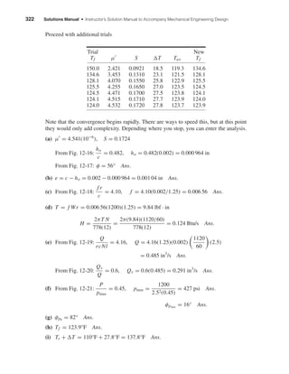
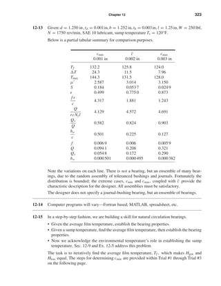
324. 324 Solutions Manual • Instructor’s Solution Manual to Accompany Mechanical Engineering Design
Trial #1:
• Choose a value of Tf .
• Find the corresponding viscosity.
• Find the Sommerfeld number.
• Find f r/c, then
Hgen =
2545
1050
W N c
f r
c
• Find Q/(rcNl) and Qs/Q. From Eq. (12–15)
T =
0.103P( f r/c)
(1 − 0.5Qs/Q)[Q/(rcNjl)]
Hloss =
¯hCR A(Tf − T∞)
1 + α
• Display Tf , S, Hgen, Hloss
Trial #2: Choose another Tf , repeating above drill.
Trial #3:
Plot the results of the first two trials.
Choose (Tf )3 from plot. Repeat the drill. Plot the results of Trial #3 on the above graph.
If you are not within 0.1°F, iterate again. Otherwise, stop, and find all the properties of
the bearing for the first clearance, cmin . See if Trumpler conditions are satisfied, and if so,
analyze ¯c and cmax .
The bearing ensemble in the current problem statement meets Trumpler’s criteria
(for nd = 2).
This adequacy assessment protocol can be used as a design tool by giving the students
additional possible bushing sizes.
b (in) tb (in)
2.254 0.004
2.004 0.004
1.753 0.003
Otherwise, the design option includes reducingl/d to save on the cost of journal machin-
ing and vender-supplied bushings.
H Hgen
Hloss, linear with Tf
(Tf)1 (Tf)3 (Tf)2
Tf
shi20396_ch12.qxd 8/29/03 2:22 PM Page 324

325. Chapter 12 325
12-16 Continue to build a skill with pressure-fed bearings, that of finding the average tempera-
ture of the fluid film. First examine the case for c = cmin
Trial #1:
• Choose an initial Tf .
• Find the viscosity.
• Find the Sommerfeld number.
• Find f r/c, ho/c, and .
• From Eq. (12-24), find T .
Tav = Ts +
T
2
• Display Tf , S, T, and Tav.
Trial #2:
• Choose another Tf . Repeat the drill, and display the second set of values for Tf ,
S, T, and Tav.
• Plot Tav vs Tf :
Trial #3:
Pick the third Tf from the plot and repeat the procedure. If(Tf )3 and(Tav)3 differ by more
than 0.1°F, plot the results for Trials #2 and #3 and try again. If they are within 0.1°F, de-
termine the bearing parameters, check the Trumpler criteria, and compare Hloss with the
lubricant’s cooling capacity.
Repeat the entire procedure for c = cmax to assess the cooling capacity for the maxi-
mum radial clearance. Finally, examine c = ¯c to characterize the ensemble of bearings.
12-17 An adequacy assessment associated with a design task is required. Trumpler’s criteria
will do.
d = 50.00+0.00
−0.05 mm, b = 50.084+0.010
−0.000 mm
SAE 30, N = 2880 rev/min or 48 rev/s, W = 10 kN
cmin =
bmin − dmax
2
=
50.084 − 50
2
= 0.042 mm
r = d/2 = 50/2 = 25 mm
r/c = 25/0.042 = 595$
l =
1
2
(55 − 5) = 25 mm
l /d = 25/50 = 0.5
p =
W
4rl
=
10(106
)
4(0.25)(0.25)
= 4000 kPa
Tav
2
1
Tf(Tf)1(Tf)2 (Tf)3
Tav ϭ Tf
shi20396_ch12.qxd 8/29/03 2:22 PM Page 325

326. 326 Solutions Manual • Instructor’s Solution Manual to Accompany Mechanical Engineering Design
Trial #1: Choose (Tf )1 = 79°C. From Fig. 12-13, µ = 13 MPa · s.
S = (5952
)
13(10−3
)(48)
4000(103)
= 0.055
From Figs. 12-18 and 12-16:
f r
c
= 2.3, = 0.85.
From Eq. (12-25), T =
978(106
)
1 + 1.5 2
( f r/c)SW2
psr4
=
978(106
)
1 + 1.5(0.85)2
2.3(0.055)(102
)
200(25)4
= 76.0°C
Tav = Ts + T/2 = 55°C + (76°C/2) = 93°C
Trial #2: Choose (Tf )2 = 100°C. From Fig. 12-13, µ = 7 MPa · s.
S = 0.055
7
13
= 0.0296
From Figs. 12-18 and 12-16:
f r
c
= 1.6, = 0.90
T =
978(106
)
1 + 1.5(0.9)2
1.6(0.0296)(102
)
200(25)4
= 26.8°C
Tav = 55°C +
26.8°C
2
= 68.4°C
Trial #3: Thus, the plot gives (Tf )3 = 85°C. From Fig. 12-13, µ = 10.8 MPa · s.
S = 0.055
10.8
13
= 0.0457
From Figs. 12-18 and 12-16:
f r
c
= 2.2, = 0.875
T =
978(106
)
1 + 1.5(0.8752)
2.2(0.0457)(102
)
200(25)4
= 58.6°C
Tav = 55°C +
58.6°C
2
= 84.3°C
Result is close. Choose ¯Tf =
85°C + 84.3°C
2
= 84.7°C
100
Tav
Tf60 70 80 90 100
(79ЊC, 93ЊC)
(79ЊC, 79ЊC)
85ЊC
(100ЊC, 68.4ЊC)
(100ЊC, 100ЊC)
90
80
70
Tav ϭ Tf
shi20396_ch12.qxd 8/29/03 2:22 PM Page 326

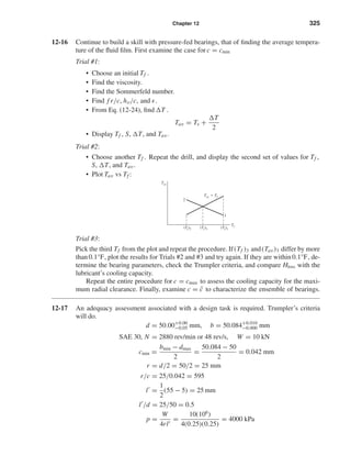
327. Chapter 12 327
Fig. 12-13: µ = 10.8 MPa · s
S = 0.055
10.8
13
= 0.0457
f r
c
= 2.23, = 0.874,
ho
c
= 0.13
T =
978(106
)
1 + 1.5(0.8742)
2.23(0.0457)(102
)
200(254)
= 59.5°C
Tav = 55°C +
59.5°C
2
= 84.7°C O.K.
From Eq. (12-22)
Qs = (1 + 1.5 2
)
πpsrc3
3µl
= [1 + 1.5(0.8742
)]
π(200)(0.0423
)(25)
3(10)(10−6)(25)
= 3334 mm3
/s
ho = 0.13(0.042) = 0.005 46 mm or 0.000 215 in
Trumpler:
ho = 0.0002 + 0.000 04(50/25.4)
= 0.000 279 in Not O.K.
Tmax = Ts + T = 55°C + 63.7°C = 118.7°C or 245.7°F O.K.
Pst = 4000 kPa or 581 psi Not O.K.
n = 1, as done Not O.K.
There is no point in proceeding further.
12-18 So far, we’ve performed elements of the design task. Now let’s do it more completely.
First, remember our viewpoint.
The values of the unilateral tolerances, tb and td, reflect the routine capabilities of the
bushing vendor and the in-house capabilities. While the designer has to live with these,
his approach should not depend on them. They can be incorporated later.
First we shall find the minimum size of the journal which satisfies Trumpler’s con-
straint of Pst ≤ 300 psi.
Pst =
W
2dl
≤ 300
W
2d2 l /d
≤ 300 ⇒ d ≥
W
600(l /d)
dmin =
900
2(300)(0.5)
= 1.73 in
shi20396_ch12.qxd 8/29/03 2:22 PM Page 327

328. 328 Solutions Manual • Instructor’s Solution Manual to Accompany Mechanical Engineering Design
In this problem we will take journal diameter as the nominal value and the bushing bore
as a variable. In the next problem, we will take the bushing bore as nominal and the jour-
nal diameter as free.
To determine where the constraints are, we will set tb = td = 0, and thereby shrink
the design window to a point.
We set d = 2.000 in
b = d + 2cmin = d + 2c
nd = 2 (This makes Trumpler’s nd ≤ 2 tight)
and construct a table.
c b d ¯Tf
*
Tmax ho Pst Tmax n fom
0.0010 2.0020 2 215.50 312.0 × × −5.74
0.0011 2.0022 2 206.75 293.0 × −6.06
0.0012 2.0024 2 198.50 277.0 × −6.37
0.0013 2.0026 2 191.40 262.8 × −6.66
0.0014 2.0028 2 185.23 250.4 × −6.94
0.0015 2.0030 2 179.80 239.6 × −7.20
0.0016 2.0032 2 175.00 230.1 × −7.45
0.0017 2.0034 2 171.13 220.3 × −7.65
0.0018 2.0036 2 166.92 213.9 −7.91
0.0019 2.0038 2 163.50 206.9 −8.12
0.0020 2.0040 2 160.40 200.6 −8.32
*Sample calculation for the first entry of this column.
Iteration yields: ¯Tf = 215.5°F
With ¯Tf = 215.5°F, from Table 12-1
µ = 0.0136(10−6
) exp[1271.6/(215.5 + 95)] = 0.817(10−6
) reyn
N = 3000/60 = 50 rev/s, P =
900
4
= 225 psi
S =
1
0.001
2
0.817(10−6
)(50)
225
= 0.182
From Figs. 12-16 and 12-18: = 0.7, f r/c = 5.5
Eq. (12–24):
TF =
0.0123(5.5)(0.182)(9002
)
[1 + 1.5(0.72)](30)(14)
= 191.6°F
Tav = 120°F +
191.6°F
2
= 215.8°F
.
= 215.5°F
For the nominal 2-in bearing, the various clearances show that we have been in contact
with the recurving of (ho)min. The figure of merit (the parasitic friction torque plus the
pumping torque negated) is best at c = 0.0018 in. For the nominal 2-in bearing, we will
place the top of the design window at cmin = 0.002 in, and b = d + 2(0.002) = 2.004 in.
At this point, add the b and d unilateral tolerances:
d = 2.000+0.000
−0.001 in, b = 2.004+0.003
−0.000 in
shi20396_ch12.qxd 8/29/03 2:22 PM Page 328

329. Chapter 12 329
Now we can check the performance at cmin , ¯c, and cmax . Of immediate interest is the fom
of the median clearance assembly, −9.82, as compared to any other satisfactory bearing
ensemble.
If a nominal 1.875 in bearing is possible, construct another table with tb = 0 and
td = 0.
c b d ¯Tf Tmax ho Pst Tmax fos fom
0.0020 1.879 1.875 157.2 194.30 × −7.36
0.0030 1.881 1.875 138.6 157.10 −8.64
0.0035 1.882 1.875 133.5 147.10 −9.05
0.0040 1.883 1.875 130.0 140.10 −9.32
0.0050 1.885 1.875 125.7 131.45 −9.59
0.0055 1.886 1.875 124.4 128.80 −9.63
0.0060 1.887 1.875 123.4 126.80 × −9.64
The range of clearance is 0.0030 < c < 0.0055 in. That is enough room to fit in our de-
sign window.
d = 1.875+0.000
−0.001 in, b = 1.881+0.003
−0.000 in
The ensemble median assembly has fom = −9.31.
We just had room to fit in a design window based upon the (ho)min constraint. Further
reduction in nominal diameter will preclude any smaller bearings. A table constructed for a
d = 1.750 in journal will prove this.
We choose the nominal 1.875-in bearing ensemble because it has the largest figure
of merit. Ans.
12-19 This is the same as Prob. 12-18 but uses design variables of nominal bushing bore b and
radial clearance c.
The approach is similar to that of Prob. 12-18 and the tables will change slightly. In the
table for a nominal b = 1.875 in, note that at c = 0.003 the constraints are “loose.” Set
b = 1.875 in
d = 1.875 − 2(0.003) = 1.869 in
For the ensemble
b = 1.875+0.003
−0.001, d = 1.869+0.000
−0.001
Analyze at cmin = 0.003, ¯c = 0.004 in and cmax = 0.005 in
At cmin = 0.003 in: ¯Tf = 138.4, µ = 3.160, S = 0.0297, Hloss = 1035 Btu/h and the
Trumpler conditions are met.
At ¯c = 0.004 in: ¯Tf = 130°F, µ = 3.872, S = 0.0205, Hloss = 1106 Btu/h, fom =
−9.246 and the Trumpler conditions are O.K.
At cmax = 0.005 in: ¯Tf = 125.68°F, µ = 4.325 µreyn, S = 0.014 66, Hloss =
1129 Btu/h and the Trumpler conditions are O.K.
The ensemble figure of merit is slightly better; this bearing is slightly smaller. The lubri-
cant cooler has sufficient capacity.
shi20396_ch12.qxd 8/29/03 2:22 PM Page 329

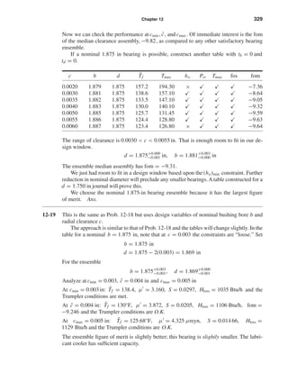
330. 330 Solutions Manual • Instructor’s Solution Manual to Accompany Mechanical Engineering Design
12-20 From Table 12-1, Seireg and Dandage, µ0 = 0.0141(106
) reyn and b = 1360.0
µ(µreyn) = 0.0141 exp[1360/(T + 95)] (T in °F)
= 0.0141 exp[1360/(1.8C + 127)] (C in °C)
µ(MPa · s) = 6.89(0.0141) exp[1360/(1.8C + 127)] (C in °C)
For SAE 30 at 79°C
µ = 6.89(0.0141) exp{1360/[1.8(79) + 127]}
= 15.2 MPa · s Ans.
12-21 Originally
d = 2.000+0.000
−0.001 in, b = 2.005+0.003
−0.000 in
Doubled,
d = 4.000+0.000
−0.002 in, b = 4.010+0.006
−0.000
The radial load quadrupled to 3600 lbf when the analyses for parts (a) and (b) were carried
out. Some of the results are:
Trumpler
Part ¯c µ S ¯Tf f r/c Qs ho/c Hloss ho ho f
(a) 0.007 3.416 0.0310 135.1 0.1612 6.56 0.1032 0.897 9898 0.000722 0.000360 0.00567
(b) 0.0035 3.416 0.0310 135.1 0.1612 0.870 0.1032 0.897 1237 0.000361 0.000280 0.00567
The side flow Qs differs because there is a c3
term and consequently an 8-fold increase.
Hloss is related by a9898/1237 or an 8-fold increase. The existingho is related by a 2-fold
increase. Trumpler’s (ho)min is related by a 1.286-fold increase
fom = −82.37 for double size
fom = −10.297 for original size} an 8-fold increase for double-size
12-22 From Table 12-8: K = 0.6(10−10
) in3
· min/(lbf · ft · h). P = 500/[(1)(1)] = 500 psi,
V = π DN/12 = π(1)(200)/12 = 52.4 ft/min
Tables 12-10 and 12-11: f1 = 1.8, f2 = 1
Table 12-12: PVmax = 46 700 psi · ft/min, Pmax = 3560 psi, Vmax = 100 ft/min
Pmax =
4
π
F
DL
=
4(500)
π(1)(1)
= 637 psi < 3560 psi O.K.
P =
F
DL
= 500 psi V = 52.4 ft/min
PV = 500(52.4) = 26 200 psi · ft/min < 46 700 psi · ft/min O.K.
shi20396_ch12.qxd 8/29/03 2:22 PM Page 330

331. Chapter 12 331
Solving Eq. (12-32) for t
t =
π DLw
4 f1 f2 K V F
=
π(1)(1)(0.005)
4(1.8)(1)(0.6)(10−10)(52.4)(500)
= 1388 h = 83 270 min
Cycles = Nt = 200(83 270) = 16.7 rev Ans.
12-23 Estimate bushing length with f1 = f2 = 1, and K = 0.6(10−10
) in3
· min/(lbf · ft · h)
Eq. (12-32): L =
1(1)(0.6)(10−10
)(2)(100)(400)(1000)
3(0.002)
= 0.80in
From Eq. (12-38), with fs = 0.03 from Table 12-9 applying nd = 2 to F
and ¯hCR = 2.7 Btu/(h · ft2
· °F)
L
.
=
720(0.03)(2)(100)(400)
778(2.7)(300 − 70)
= 3.58 in
0.80 ≤ L ≤ 3.58 in
Trial 1: Let L = 1 in, D = 1 in
Pmax =
4(2)(100)
π(1)(1)
= 255 psi < 3560 psi O.K.
P =
2(100)
1(1)
= 200 psi
V =
π(1)(400)
12
= 104.7 ft/min > 100 ft/min Not O.K.
Trial 2: Try D = 7/8 in, L = 1 in
Pmax =
4(2)(100)
π(7/8)(1)
= 291 psi < 3560 psi O.K.
P =
2(100)
7/8(1)
= 229 psi
V =
π(7/8)(400)
12
= 91.6 ft/min < 100 ft/min O.K.
PV = 229(91.6) = 20 976 psi · ft/min < 46 700 psi · ft/min O.K.
⇒ f1 = 1.3 + (1.8 − 1.3)
91.6 − 33
100 − 33
= 1.74
L = 0.80(1.74) = 1.39 in
V f1
33 1.3
91.6 f1
100 1.8
shi20396_ch12.qxd 8/29/03 2:22 PM Page 331

332. 332 Solutions Manual • Instructor’s Solution Manual to Accompany Mechanical Engineering Design
Trial 3: Try D = 7/8 in, L = 1.5 in
Pmax =
4(2)(100)
π(7/8)(1.5)
= 194 psi < 3560 psi O.K.
P =
2(100)
7/8(1.5)
= 152 psi, V = 91.6 ft/min
PV = 152(91.6) = 13 923 psi · ft/min < 46 700 psi · ft/min O.K.
D = 7/8 in, L = 1.5 in is acceptable Ans.
Suggestion: Try smaller sizes.
shi20396_ch12.qxd 8/29/03 2:22 PM Page 332

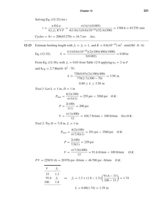
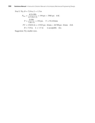
333. Chapter 13
13-1
dP = 17/8 = 2.125 in
dG =
N2
N3
dP =
1120
544
(2.125) = 4.375 in
NG = PdG = 8(4.375) = 35 teeth Ans.
C = (2.125 + 4.375)/2 = 3.25 in Ans.
13-2
nG = 1600(15/60) = 400 rev/min Ans.
p = πm = 3π mm Ans.
C = [3(15 + 60)]/2 = 112.5 mm Ans.
13-3
NG = 20(2.80) = 56 teeth Ans.
dG = NGm = 56(4) = 224 mm Ans.
dP = NPm = 20(4) = 80 mm Ans.
C = (224 + 80)/2 = 152 mm Ans.
13-4 Mesh: a = 1/P = 1/3 = 0.3333 in Ans.
b = 1.25/P = 1.25/3 = 0.4167 in Ans.
c = b − a = 0.0834 in Ans.
p = π/P = π/3 = 1.047 in Ans.
t = p/2 = 1.047/2 = 0.523 in Ans.
Pinion Base-Circle: d1 = N1/P = 21/3 = 7 in
d1b = 7 cos 20° = 6.578 in Ans.
Gear Base-Circle: d2 = N2/P = 28/3 = 9.333 in
d2b = 9.333 cos 20° = 8.770 in Ans.
Base pitch: pb = pc cos φ = (π/3) cos 20° = 0.984 in Ans.
Contact Ratio: mc = Lab/pb = 1.53/0.984 = 1.55 Ans.
See the next page for a drawing of the gears and the arc lengths.
shi20396_ch13.qxd 8/29/03 12:16 PM Page 333

334. 334 Solutions Manual • Instructor’s Solution Manual to Accompany Mechanical Engineering Design
13-5
(a) AO =
2.333
2
2
+
5.333
2
2 1/2
= 2.910 in Ans.
(b) γ = tan−1
(14/32) = 23.63° Ans.
= tan−1
(32/14) = 66.37° Ans.
(c) dP = 14/6 = 2.333 in,
dG = 32/6 = 5.333 in Ans.
(d) From Table 13-3, 0.3AO = 0.873 in and 10/P = 10/6 = 1.67
0.873 < 1.67 ∴ F = 0.873 in Ans.
13-6
(a) pn = π/5 = 0.6283 in
pt = pn/cos ψ = 0.6283/cos 30° = 0.7255 in
px = pt/tan ψ = 0.7255/tan 30° = 1.25 in
30Њ
P G
2
1
3
"
5
1
3
"
AO
⌫
␥
10.5Њ
Arc of approach ϭ 0.87 in Ans.
Arc of recess ϭ 0.77 in Ans.
Arc of action ϭ 1.64 in Ans.
Lab ϭ 1.53 in
10Њ
O2
O1
14Њ 12.6Њ
P
BA
shi20396_ch13.qxd 8/29/03 12:16 PM Page 334

335. Chapter 13 335
(b) pnb = pn cos φn = 0.6283 cos 20° = 0.590 in Ans.
(c) Pt = Pn cos ψ = 5 cos 30° = 4.33 teeth/in
φt = tan−1
(tan φn/cos ψ) = tan−1
(tan 20°/cos 30◦
) = 22.8° Ans.
(d) Table 13-4:
a = 1/5 = 0.200 in Ans.
b = 1.25/5 = 0.250 in Ans.
dP =
17
5 cos 30°
= 3.926 in Ans.
dG =
34
5 cos 30°
= 7.852 in Ans.
13-7
φn = 14.5°, Pn = 10 teeth/in
(a) pn = π/10 = 0.3142 in Ans.
pt =
pn
cos ψ
=
0.3142
cos 20°
= 0.3343 in Ans.
px =
pt
tan ψ
=
0.3343
tan 20°
= 0.9185 in Ans.
(b) Pt = Pn cos ψ = 10 cos 20° = 9.397 teeth/in
φt = tan−1 tan 14.5°
cos 20°
= 15.39° Ans.
(c) a = 1/10 = 0.100 in Ans.
b = 1.25/10 = 0.125 in Ans.
dP =
19
10 cos 20°
= 2.022 in Ans.
dG =
57
10 cos 20°
= 6.066 in Ans.
G
20Њ
P
shi20396_ch13.qxd 8/29/03 12:16 PM Page 335

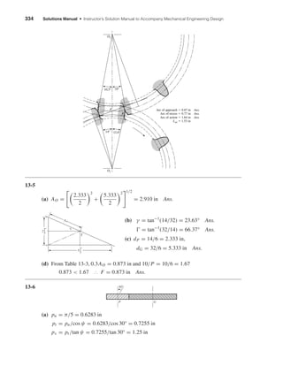
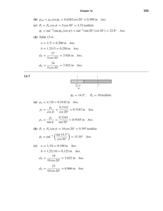
336. 336 Solutions Manual • Instructor’s Solution Manual to Accompany Mechanical Engineering Design
13-8 From Ex. 13-1, a 16-tooth spur pinion meshes with a 40-tooth gear, mG = 40/16 = 2.5.
Equations (13-10) through (13-13) apply.
(a) The smallest pinion tooth count that will run with itself is found from Eq. (13-10)
NP ≥
4k
6 sin2
φ
1 + 1 + 3 sin2
φ
≥
4(1)
6 sin2
20°
1 + 1 + 3 sin2
20°
≥ 12.32 → 13 teeth Ans.
(b) The smallest pinion that will mesh with a gear ratio of mG = 2.5, from Eq. (13-11) is
NP ≥
2(1)
[1 + 2(2.5)] sin2
20°
2.5 + 2.52 + [1 + 2(2.5)] sin2
20°
≥ 14.64 → 15 pinion teeth Ans.
(c) The smallest pinion that will mesh with a rack, from Eq. (13-12)
NP ≥
4k
2 sin2
φ
=
4(1)
2 sin2
20°
≥ 17.097 → 18 teeth Ans.
(d) The largest gear-tooth count possible to mesh with this pinion, from Eq. (13-13) is
NG ≤
N2
P sin2
φ − 4k2
4k − 2NP sin2
φ
≤
132
sin2
20° − 4(1)2
4(1) − 2(13) sin2
20°
≤ 16.45 → 16 teeth Ans.
13-9 From Ex. 13-2, a 20° pressure angle, 30° helix angle, pt = 6 teeth/in pinion with 18 full
depth teeth, and φt = 21.88°.
(a) The smallest tooth count that will mesh with a like gear, from Eq. (13-21), is
NP ≥
4k cos ψ
6 sin2
φt
1 + 1 + 3 sin2
φt
≥
4(1) cos 30°
6 sin2
21.88°
1 + 1 + 3 sin2
21.88°
≥ 9.11 → 10 teeth Ans.
(b) The smallest pinion-tooth count that will run with a rack, from Eq. (13-23), is
NP ≥
4k cos ψ
2 sin2
φt
≥
4(1) cos 30◦
2 sin2
21.88°
≥ 12.47 → 13 teeth Ans.
shi20396_ch13.qxd 8/29/03 12:16 PM Page 336

337. Chapter 13 337
(c) The largest gear tooth possible, from Eq. (13-24) is
NG ≤
N2
P sin2
φt − 4k2
cos2
ψ
4k cos ψ − 2NP sin2
φt
≤
102
sin2
21.88° − 4(12
) cos2
30°
4(1) cos 30° − 2(10) sin2
21.88°
≤ 15.86 → 15 teeth Ans.
13-10 Pressure Angle: φt = tan−1 tan 20°
cos 30°
= 22.796°
Program Eq. (13-24) on a computer using a spreadsheet or code and increment NP. The
first value of NP that can be doubled is NP = 10 teeth, where NG ≤ 26.01 teeth. So NG =
20 teeth will work. Higher tooth counts will work also, for example 11:22, 12:24, etc.
Use 10:20 Ans.
13-11 Refer to Prob. 13-10 solution. The first value of NP that can be multiplied by 6 is
NP = 11 teeth where NG ≤ 93.6 teeth. So NG = 66 teeth.
Use 11:66 Ans.
13-12 Begin with the more general relation, Eq. (13-24), for full depth teeth.
NG =
N2
P sin2
φt − 4 cos2
ψ
4 cos ψ − 2NP sin2
φt
Set the denominator to zero
4 cos ψ − 2NP sin2
φt = 0
From which
sin φt =
2 cos ψ
NP
φt = sin−1 2 cos ψ
NP
For NP = 9 teeth and cos ψ = 1
φt = sin−1 2(1)
9
= 28.126° Ans.
13-13
(a) pn = πmn = 3π mm Ans.
pt = 3π/cos 25° = 10.4 mm Ans.
px = 10.4/tan 25° = 22.3 mm Ans.
18T 32T
␺ ϭ 25Њ, ␾n ϭ 20Њ, m ϭ 3 mm
shi20396_ch13.qxd 8/29/03 12:16 PM Page 337

338. 338 Solutions Manual • Instructor’s Solution Manual to Accompany Mechanical Engineering Design
(b) mt = 10.4/π = 3.310 mm Ans.
φt = tan−1 tan 20°
cos 25°
= 21.88° Ans.
(c) dP = 3.310(18) = 59.58 mm Ans.
dG = 3.310(32) = 105.92 mm Ans.
13-14 (a) The axial force of 2 on shaft a is in the negative direction. The axial force of 3 on
shaft b is in the positive direction of z. Ans.
The axial force of gear 4 on shaft b is in the positive z-direction. The axial force of
gear 5 on shaft c is in the negative z-direction. Ans.
(b) nc = n5 =
14
54
16
36
(900) = +103.7 rev/min ccw Ans.
(c) dP2 = 14/(10 cos 30°) = 1.6166 in
dG3 = 54/(10 cos 30°) = 6.2354 in
Cab =
1.6166 + 6.2354
2
= 3.926 in Ans.
dP4 = 16/(6 cos 25°) = 2.9423 in
dG5 = 36/(6 cos 25°) = 6.6203 in
Cbc = 4.781 in Ans.
13-15 e =
20
40
8
17
20
60
=
4
51
nd =
4
51
(600) = 47.06 rev/min cw Ans.
5
4
c
b
z
a
3
z
2
b
shi20396_ch13.qxd 8/29/03 12:16 PM Page 338

339. Chapter 13 339
13-16
e =
6
10
18
38
20
48
3
36
=
3
304
na =
3
304
(1200) = 11.84 rev/min cw Ans.
13-17
(a) nc =
12
40
·
1
1
(540) = 162 rev/min cw about x. Ans.
(b) dP = 12/(8 cos 23°) = 1.630 in
dG = 40/(8 cos 23°) = 5.432 in
dP + dG
2
= 3.531 in Ans.
(c) d =
32
4
= 8 in at the large end of the teeth. Ans.
13-18 (a) The planet gears act as keys and the wheel speeds are the same as that of the ring gear.
Thus
nA = n3 = 1200(17/54) = 377.8 rev/min Ans.
(b) nF = n5 = 0, nL = n6, e = −1
−1 =
n6 − 377.8
0 − 377.8
377.8 = n6 − 377.8
n6 = 755.6 rev/min Ans.
Alternatively, the velocity of the center of gear 4 is v4c ∝ N6n3 . The velocity of the
left edge of gear 4 is zero since the left wheel is resting on the ground. Thus, the ve-
locity of the right edge of gear 4 is2v4c ∝ 2N6n3. This velocity, divided by the radius
of gear 6 ∝ N6, is angular velocity of gear 6–the speed of wheel 6.
∴ n6 =
2N6n3
N6
= 2n3 = 2(377.8) = 755.6 rev/min Ans.
(c) The wheel spins freely on icy surfaces, leaving no traction for the other wheel. The
car is stalled. Ans.
13-19 (a) The motive power is divided equally among four wheels instead of two.
(b) Locking the center differential causes 50 percent of the power to be applied to the
rear wheels and 50 percent to the front wheels. If one of the rear wheels, rests on
a slippery surface such as ice, the other rear wheel has no traction. But the front
wheels still provide traction, and so you have two-wheel drive. However, if the rear
differential is locked, you have 3-wheel drive because the rear-wheel power is now
distributed 50-50.
shi20396_ch13.qxd 8/29/03 12:16 PM Page 339

340. 340 Solutions Manual • Instructor’s Solution Manual to Accompany Mechanical Engineering Design
13-20 Let gear 2 be first, then nF = n2 = 0. Let gear 6 be last, then nL = n6 = −12 rev/min.
e =
20
30
16
34
=
16
51
, e =
nL − nA
nF − nA
(0 − nA)
16
51
= −12 − nA
nA =
−12
35/51
= −17.49 rev/min (negative indicates cw) Ans.
Alternatively, since N ∝ r, let v = Nn (crazy units).
v = N6n6 N6 = 20 + 30 − 16 = 34 teeth
vA
N4
=
v
N4 − N5
⇒ vA =
N4 N6n6
N4 − N5
nA =
vA
N2 + N4
=
N4 N6n6
(N2 + N4)(N4 − N5)
=
30(34)(12)
(20 + 30)(30 − 16)
= 17.49 rev/min cw Ans.
13-21 Let gear 2 be first, then nF = n2 = 180 rev/min. Let gear 6 be last, then nL = n6 = 0.
e =
20
30
16
34
=
16
51
, e =
nL − nA
nF − nA
(180 − nA)
16
51
= (0 − nA)
nA = −
16
35
180 = −82.29 rev/min
The negative sign indicates opposite n2 ∴ nA = 82.29 rev/min cw Ans.
Alternatively, since N ∝ r, let v = Nn (crazy units).
vA
N5
=
v
N4 − N5
=
N2n2
N4 − N5
vA =
N5 N2n2
N4 − N5
nA =
vA
N2 + N4
=
N5 N2n2
(N2 + N4)(N4 − N5)
=
16(20)(180)
(20 + 30)(30 − 16)
= 82.29 rev/min cw Ans.
45
v ϭ 0
v ϭ N2n2
N2
vA
2
4
5
v
v ϭ 0
vA
2
shi20396_ch13.qxd 8/29/03 12:16 PM Page 340

341. Chapter 13 341
13-22 N5 = 12 + 2(16) + 2(12) = 68 teeth Ans.
Let gear 2 be first, nF = n2 = 320 rev/min. Let gear 5 be last, nL = n5 = 0
e =
12
16
16
12
12
68
=
3
17
, e =
nL − nA
nF − nA
320 − nA =
17
3
(0 − nA)
nA = −
3
14
(320) = −68.57 rev/min
The negative sign indicates opposite of n2 ∴ nA = 68.57 rev/min cw Ans.
Alternatively,
nA =
n2 N2
2(N3 + N4)
=
320(12)
2(16 + 12)
= 68.57 rev/min cw Ans.
13-23 Let nF = n2 then nL = n7 = 0.
e = −
24
18
18
30
36
54
= −
8
15
e =
nL − n5
nF − n5
= −
8
15
0 − 5
n2 − 5
= −
8
15
⇒ n2 = 5 +
15
8
(5) = 14.375 turns in same direction
13-24 (a) Let nF = n2 = 0, then nL = n5.
e =
99
100
101
100
=
9999
10 000
, e =
nL − nA
nF − nA
=
nL − nA
0 − nA
nL − nA = −enA
nL = nA(−e + 1)
nL
nA
= 1 − e = 1 −
9999
10 000
=
1
10 000
= 0.0001 Ans.
(b) d4 =
N4
P
=
101
10
= 10.1 in
d5 =
100
10
= 10 in
dhousing > 2 d4 +
d5
2
= 2 10.1 +
10
2
= 30.2 in Ans.
v ϭ 0
nA(N2 ϩ N3)
v ϭ n2N2
2nA(N2 ϩ 2N3 ϩ N4) ϭ n2N2 ϩ 2nA(N2 ϩ N3)
2nA(N2 ϩ 2N3 ϩ N4) Ϫ 2nA(N2 ϩ N3) ϭ n2N2
nA(N2 ϩ 2N3 ϩ N4)
shi20396_ch13.qxd 8/29/03 12:16 PM Page 341

342. 342 Solutions Manual • Instructor’s Solution Manual to Accompany Mechanical Engineering Design
13-25 n2 = nb = nF, nA = na, nL = n5 = 0
e = −
21
444
=
nL − nA
nF − nA
−
21
444
(nF − nA) = 0 − nA
With shaft b as input
−
21
444
nF +
21
444
nA +
444
444
nA = 0
nA
nF
=
na
nb
=
21
465
na =
21
465
nb, in the same direction as shaft b, the input. Ans.
Alternatively,
vA
N4
=
n2 N2
N3 + N4
vA =
n2 N2 N4
N3 + N4
na = nA =
vA
N2 + N3
=
n2 N2 N4
(N2 + N3)(N3 + N4)
=
18(21)(nb)
(18 + 72)(72 + 21)
=
21
465
nb in the same direction as b Ans.
13-26 nF = n2 = na, nL = n6 = 0
e = −
24
18
22
64
= −
11
24
, e =
nL − nA
nF − nA
=
0 − nb
na − nb
−
11
24
=
0 − nb
na − nb
⇒
nb
na
=
11
35
Ans.
Yes, both shafts rotate in the same direction. Ans.
Alternatively,
vA
N5
=
n2 N2
N3 + N5
=
N2
N3 + N5
na, vA =
N2 N5
N3 + N5
na
nA = nb =
vA
N2 + N3
=
N2 N5
(N2 + N3)(N3 + N5)
na
nb
na
=
24(22)
(24 + 18)(22 + 18)
=
11
35
Ans.
nb rotates ccw ∴ Yes Ans.
13-27 n2 = nF = 0, nL = n5 = nb, nA = na
e = +
20
24
20
24
=
25
36
3
5
v ϭ 0
vA
n2N2
2
3
4
2
v ϭ 0
vA
n2N2
shi20396_ch13.qxd 8/29/03 12:16 PM Page 342

343. Chapter 13 343
25
36
=
nb − na
0 − na
nb
na
=
11
36
Ans.
Same sense, therefore shaft b rotates in the same direction as a. Ans.
Alternatively,
v5
N3 − N4
=
(N2 + N3)na
N3
v5 =
(N2 + N3)(N3 − N4)n
N3
nb =
v5
N5
=
(N2 + N3)(N3 − N4)na
N3 N5
nb
na
=
(20 + 24)(24 − 20)
24(24)
=
11
36
same sense Ans.
13-28 (a) ω = 2πn/60
H = Tω = 2πTn/60 (T in N · m, H in W)
So T =
60H(103
)
2πn
= 9550H/n (H in kW, n in rev/min)
Ta =
9550(75)
1800
= 398 N · m
r2 =
mN2
2
=
5(17)
2
= 42.5 mm
So
Ft
32 =
Ta
r2
=
398
42.5
= 9.36 kN
F3b = −Fb3 = 2(9.36) = 18.73 kN in the positive x-direction. Ans.
See the figure in part (b) on the following page.
9.36
2
a
Ta2
398 N•m
Ft
32
3
4
v5
v ϭ 0
(N2 ϩ N3)na
shi20396_ch13.qxd 8/29/03 12:16 PM Page 343

344. 344 Solutions Manual • Instructor’s Solution Manual to Accompany Mechanical Engineering Design
(b) r4 =
mN4
2
=
5(51)
2
= 127.5 mm
Tc4 = 9.36(127.5) = 1193 N · m ccw
∴ T4c = 1193 N · m cw Ans.
Note: The solution is independent of the pressure angle.
13-29
d =
N
6
d2 = 4 in, d4 = 4 in, d5 = 6 in, d6 = 24 in
e =
24
24
24
36
36
144
= 1/6, nP = n2 = 1000 rev/min
nL = n6 = 0
e =
nL − nA
nF − nA
=
0 − nA
1000 − nA
nA = −200 rev/min
2 4
5
6
9.36
4
c
Tc4 ϭ 1193
b
9.36
O
3
Ft
43
9.36
18.73
Ft
23
Fb3
shi20396_ch13.qxd 8/29/03 12:16 PM Page 344

345. Chapter 13 345
Input torque: T2 =
63 025H
n
T2 =
63 025(25)
1000
= 1576 lbf · in
For 100 percent gear efficiency
Tarm =
63 025(25)
200
= 7878 lbf · in
Gear 2
Wt
=
1576
2
= 788 lbf
Fr
32 = 788 tan 20° = 287 lbf
Gear 4
FA4 = 2Wt
= 2(788) = 1576 lbf
Gear 5
Arm
Tout = 1576(9) − 1576(4) = 7880 lbf · in Ans.
13-30 Given: P = 2 teeth/in, nP = 1800 rev/min cw, N2 = 18T, N3 = 32T, N4 = 18T,
N5 = 48T.
Pitch Diameters: d2 = 18/2 = 9 in; d3 = 32/2 = 16 in; d4 = 18/2 = 9 in; d5 =
48/2 = 24 in.
4" 5"
1576 lbf
1576 lbf
Tout
ϩϩϩ
5 Wt
ϭ 788 lbf
Fr
ϭ 287 lbf
2Wt
ϭ 1576 lbf
Wt
Fr
4
n4
FA4
Wt
Wt
Fr
Fr
2
T2 ϭ 1576 lbf•inn2
Ft
a2
Wt
Fr
a2 Fr
42
shi20396_ch13.qxd 8/29/03 12:16 PM Page 345

346. 346 Solutions Manual • Instructor’s Solution Manual to Accompany Mechanical Engineering Design
Gear 2
Ta2 = 63 025(200)/1800 = 7003 lbf · in
Wt
= 7003/4.5 = 1556 lbf
Wr
= 1556 tan 20° = 566 lbf
Gears 3 and 4
Wt
(4.5) = 1556(8), Wt
= 2766 lbf
Wr
= 2766 tan 20◦
= 1007 lbf
Ans.
13-31 Given: P = 5 teeth/in, N2 = 18T, N3 = 45T, φn = 20°, H = 32 hp, n2 =
1800 rev/min.
Gear 2
Tin =
63 025(32)
1800
= 1120 lbf · in
dP =
18
5
= 3.600 in
dG =
45
5
= 9.000 in
Wt
32 =
1120
3.6/2
= 622 lbf
Wr
32 = 622 tan 20° = 226 lbf
Ft
a2 = Wt
32 = 622 lbf, Fr
a2 = Wr
32 = 226 lbf
Fa2 = (6222
+ 2262
)1/2
= 662 lbf
Each bearing on shaft a has the same radial load of RA = RB = 662/2 = 331lbf.
2
a
Tin
Wt
32
Wr
32
Fr
a2
Ft
a2
b
3
4
y
x
Wr
ϭ 566 lbf
Wt
ϭ 1556 lbf
Wt
ϭ 2766 lbf
Wr
ϭ 1007 lbf
2
a
Wt
ϭ 1556 lbf
Wr
ϭ 566 lbf
Ta2 ϭ 7003 lbf•in
shi20396_ch13.qxd 8/29/03 12:16 PM Page 346

347. Chapter 13 347
Gear 3
Wt
23 = Wt
32 = 622 lbf
Wr
23 = Wr
32 = 226 lbf
Fb3 = Fb2 = 662 lbf
RC = RD = 662/2 = 331 lbf
Each bearing on shaft b has the same radial load which is equal to the radial load of bear-
ings, A and B. Thus, all four bearings have the same radial load of 331 lbf. Ans.
13-32 Given: P = 4 teeth/in, φn = 20◦
, NP = 20T, n2 = 900 rev/min.
d2 =
NP
P
=
20
4
= 5.000 in
Tin =
63 025(30)(2)
900
= 4202 lbf · in
Wt
32 = Tin/(d2/2) = 4202/(5/2) = 1681 lbf
Wr
32 = 1681 tan 20◦
= 612 lbf
The motor mount resists the equivalent forces and torque. The radial force due to torque
Fr
=
4202
14(2)
= 150 lbf
Forces reverse with rotational
sense as torque reverses.
C
D
A
B
150
14"
150
150
4202 lbf•in
150
y
2 612 lbf
4202 lbf•in
1681 lbf
z
Equivalent
y
z 2
Wt
32 ϭ 1681 lbf
Wr
32 ϭ 612 lbf
Load on 2
due to 3
3
2
y
x
y
z
3
Tout ϭ Wt
23r3
ϭ 2799 lbf•in
b Fb
t
3
Wt
23
Wr
23
Fb
r
3
shi20396_ch13.qxd 8/29/03 12:16 PM Page 347

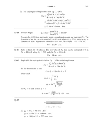
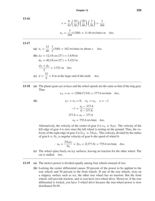
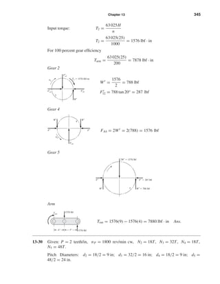
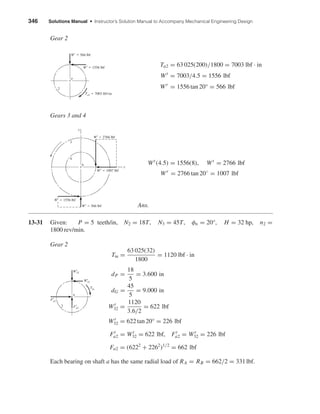
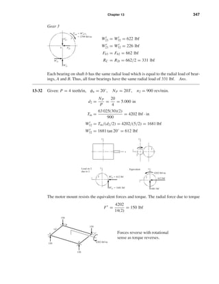
348. 348 Solutions Manual • Instructor’s Solution Manual to Accompany Mechanical Engineering Design
The compressive loads at A and D are absorbed by the base plate, not the bolts. For Wt
32 ,
the tensions in C and D are
MAB = 0 1681(4.875 + 15.25) − 2F(15.25) = 0 F = 1109 lbf
If Wt
32 reverses, 15.25 in changes to 13.25 in, 4.815 in changes to 2.875 in, and the forces
change direction. For A and B,
1681(2.875) − 2F1(13.25) = 0 ⇒ F1 = 182.4 lbf
For Wr
32
M = 612(4.875 + 11.25/2) = 6426 lbf · in
a = (14/2)2 + (11.25/2)2 = 8.98 in
F2 =
6426
4(8.98)
= 179 lbf
At C and D, the shear forces are:
FS1 = [153 + 179(5.625/8.98)]2 + [179(7/8.98)]2
= 300 lbf
At A and B, the shear forces are:
FS2 = [153 − 179(5.625/8.98)]2 + [179(7/8.98)]2
= 145 lbf
C
a
D
153 lbf
153 lbf
F2
F2F2
F2
612
4
ϭ 153 lbf
4.875
11.25
14
612 lbf
153 lbf
B
C
1681 lbf4.87515.25"
F
F
D
F1
F1
A
shi20396_ch13.qxd 8/29/03 12:16 PM Page 348

349. Chapter 13 349
The shear forces are independent of the rotational sense.
The bolt tensions and the shear forces for cw rotation are,
Tension (lbf) Shear (lbf)
A 0 145
B 0 145
C 1109 300
D 1109 300
For ccw rotation,
Tension (lbf) Shear (lbf)
A 182 145
B 182 145
C 0 300
D 0 300
13-33 Tin = 63 025H/n = 63 025(2.5)/240 = 656.5 lbf · in
Wt
= T/r = 656.5/2 = 328.3 lbf
γ = tan−1
(2/4) = 26.565°
= tan−1
(4/2) = 63.435°
a = 2 + (1.5 cos 26.565°)/2 = 2.67 in
Wr
= 328.3 tan 20° cos 26.565° = 106.9 lbf
Wa
= 328.3 tan 20° sin 26.565° = 53.4 lbf
W = 106.9i − 53.4j + 328.3k lbf
RAG = −2i + 5.17j, RAB = 2.5j
M4 = RAG × W + RAB × FB + T = 0
Solving gives
RAB × FB = 2.5Fz
Bi − 2.5Fx
Bk
RAG × W = 1697i + 656.6j − 445.9k
So
(1697i + 656.6j − 445.9k) + 2.5Fz
Bi − 2.5Fx
Bk + Tj = 0
Fz
B = −1697/2.5 = −678.8 lbf
T = −656.6 lbf · in
Fx
B = −445.9/2.5 = −178.4 lbf
y
2
2
1
2
B
A
G
WtWr
Wa
Tin
Not to scale
xz
a
F
y
A
Fz
A
Fz
B
Fx
A
Fx
B
shi20396_ch13.qxd 8/29/03 12:16 PM Page 349

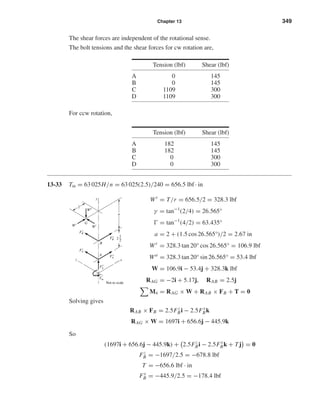
350. 350 Solutions Manual • Instructor’s Solution Manual to Accompany Mechanical Engineering Design
So
FB = [(−678.8)2
+ (−178.4)2
]1/2
= 702 lbf Ans.
FA = −(FB + W)
= −(−178.4i − 678.8k + 106.9i − 53.4j + 328.3k)
= 71.5i + 53.4j + 350.5k
FA (radial) = (71.52
+ 350.52
)1/2
= 358 lbf Ans.
FA (thrust) = 53.4 lbf Ans.
13-34
d2 = 15/10 = 1.5 in, Wt
= 30 lbf, d3 =
25
10
= 2.5 in
γ = tan−1 0.75
1.25
= 30.96°, = 59.04°
DE =
9
16
+ 0.5 cos 59.04° = 0.8197 in
Wr
= 30 tan 20° cos 59.04° = 5.617 lbf
Wa
= 30 tan 20° sin 59.04° = 9.363 lbf
W = −5.617i − 9.363j + 30k
RDG = 0.8197j + 1.25i
RDC = −0.625j
MD = RDG × W + RDC × FC + T = 0
RDG × W = 24.591i − 37.5j − 7.099k
RDC × FC = −0.625Fz
Ci + 0.625Fx
Ck
T = 37.5 lbf · in Ans.
FC = 11.4i + 39.3k lbf Ans.
FC = (11.42
+ 39.32
)1/2
= 40.9 lbf Ans.
F = 0 FD = −5.78i + 9.363j − 69.3k lbf
FD (radial) = [(−5.78)2
+ (−69.3)2
]1/2
= 69.5 lbf Ans.
FD (thrust) = Wa
= 9.363 lbf Ans.
Wr
Wa
Wt
z
C
D
E
G
x
y
5"
8
0.8197"
1.25"
Not to scale
Fx
D
Fz
D
Fx
C Fz
C
F
y
D
1.25
0.75
␥
shi20396_ch13.qxd 8/29/03 12:16 PM Page 350

351. Chapter 13 351
13-35 Sketch gear 2 pictorially.
Pt = Pn cos ψ = 4 cos 30° = 3.464 teeth/in
φt = tan−1 tan φn
cos ψ
= tan−1 tan 20°
cos 30°
= 22.80°
Sketch gear 3 pictorially,
dP =
18
3.464
= 5.196 in
Pinion (Gear 2)
Wr
= Wt
tan φt = 800 tan 22.80° = 336 lbf
Wa
= Wt
tan ψ = 800 tan 30° = 462 lbf
W = −336i − 462j + 800k lbf Ans.
W = [(−336)2
+ (−462)2
+ 8002
]1/2
= 983 lbf Ans.
Gear 3
W = 336i + 462j − 800k lbf Ans.
W = 983 lbf Ans.
dG =
32
3.464
= 9.238 in
TG = Wt
r = 800(9.238) = 7390 lbf · in
13-36 From Prob. 13-35 solution,
Notice that the idler shaft reaction contains a couple tending to turn the shaft end-over-
end. Also the idler teeth are bent both ways. Idlers are more severely loaded than other
gears, belying their name. Thus be cautious.
800
336
462
4
800800
336336
4623
462
800
2
336
462
Wa
TG
Wr
Wt
x
3
yz
Wa
Wr
T
Wt
x
y
z
2
shi20396_ch13.qxd 8/29/03 12:16 PM Page 351

352. 352 Solutions Manual • Instructor’s Solution Manual to Accompany Mechanical Engineering Design
13-37
Gear 3:
Pt = Pn cos ψ = 7 cos 30° = 6.062 teeth/in
tan φt =
tan 20°
cos 30°
= 0.4203, φt = 22.8°
d3 =
54
6.062
= 8.908 in
Wt
= 500 lbf
Wa
= 500 tan 30° = 288.7 lbf
Wr
= 500 tan 22.8° = 210.2 lbf
W3 = 210.2i + 288.7j − 500k lbf Ans.
Gear 4:
d4 =
14
6.062
= 2.309 in
Wt
= 500
8.908
2.309
= 1929 lbf
Wa
= 1929 tan 30° = 1114 lbf
Wr
= 1929 tan 22.8° = 811 lbf
W4 = −811i + 1114j − 1929k lbf Ans.
13-38
Pt = 6 cos 30° = 5.196 teeth/in
d3 =
42
5.196
= 8.083 in
φt = 22.8°
d2 =
16
5.196
= 3.079 in
T2 =
63 025(25)
1720
= 916 lbf · in
Wt
=
T
r
=
916
3.079/2
= 595 lbf
Wa
= 595 tan 30° = 344 lbf
Wr
= 595 tan 22.8° = 250 lbf
W = 344i + 250j + 595k lbf
RDC = 6i, RDG = 3i − 4.04j
T3
C
AB
D
T2
y
3
2
x
z
y
x
Wt
Wr
Wa
Wt
Wr
Wa
r4
r3
shi20396_ch13.qxd 8/29/03 12:16 PM Page 352

353. Chapter 13 353
MD = RDC × FC + RDG × W + T = 0 (1)
RDG × W = −2404i − 1785j + 2140k
RDC × FC = −6Fz
Cj + 6F
y
Ck
Substituting and solving Eq. (1) gives
T = 2404i lbf · in
Fz
C = −297.5 lbf
F
y
C = −356.7 lbf
F = FD + FC + W = 0
Substituting and solving gives
Fx
C = −344 lbf
F
y
D = 106.7 lbf
Fz
D = −297.5 lbf
So
FC = −344i − 356.7j − 297.5k lbf Ans.
FD = 106.7j − 297.5k lbf Ans.
13-39 Pt = 8 cos 15° = 7.727 teeth/in
y
2
z
x
a
Fa
a2
Ft
a2
Fr
a2
Fa
32
Fr
32
Ft
32
G
C
D
x
z
y
Wr
Wa
Wt
4.04"
3"
3"
F
y
C
Fx
C
Fz
C
Fz
T
D
F
y
D
shi20396_ch13.qxd 8/29/03 12:16 PM Page 353

354. 354 Solutions Manual • Instructor’s Solution Manual to Accompany Mechanical Engineering Design
d2 = 16/7.727 = 2.07 in
d3 = 36/7.727 = 4.66 in
d4 = 28/7.727 = 3.62 in
T2 =
63 025(7.5)
1720
= 274.8 lbf · in
Wt
=
274.8
2.07/2
= 266 lbf
Wr
= 266 tan 20° = 96.8 lbf
Wa
= 266 tan 15° = 71.3 lbf
F2a = −266i − 96.8j − 71.3k lbf Ans.
F3b = (266 − 96.8)i − (266 − 96.8)j
= 169i − 169j lbf Ans.
F4c = 96.8i + 266j + 71.3k lbf Ans.
13-40
d2 =
N
Pn cos ψ
=
14
8 cos 30°
= 2.021 in, d3 =
36
8 cos 30°
= 5.196 in
d4 =
15
5 cos 15°
= 3.106 in, d5 =
45
5 cos 15°
= 9.317 in
C
x
y
z
b
Ft
23
Fr
23
Fa
23
Ft
54
Fa
54
Fr
54
D
G
H
3"
2"
3
2.6"R
1.55"R
4
3
1"
2
F
y
DFx
D
Fx
C
F
y
C
Fz
D
y
Fr
43
Fx
b3
F
y
b3
Fa
23
Fr
23
Ft
23
Ft
43
Fa
43
3
Fb3
z
x
b
y
Ft
c4
Fr
c4
Fa
c4
4
Fa
34
Fr
34
Ft
34
z
x
c
shi20396_ch13.qxd 8/29/03 12:16 PM Page 354

355. Chapter 13 355
For gears 2 and 3: φt = tan−1
(tan φn/cos ψ) = tan−1
(tan 20°/cos 30◦
) = 22.8°,
For gears 4 and 5: φt = tan−1
(tan 20°/cos 15°) = 20.6°,
Ft
23 = T2/r = 1200/(2.021/2) = 1188 lbf
Ft
54 = 1188
5.196
3.106
= 1987 lbf
Fr
23 = Ft
23 tan φt = 1188 tan 22.8° = 499 lbf
Fr
54 = 1986 tan 20.6° = 746 lbf
Fa
23 = Ft
23 tan ψ = 1188 tan 30° = 686 lbf
Fa
54 = 1986 tan 15° = 532 lbf
Next, designate the points of action on gears 4 and 3, respectively, as points G and H,
as shown. Position vectors are
RCG = 1.553j − 3k
RC H = −2.598j − 6.5k
RC D = −8.5k
Force vectors are
F54 = −1986i − 748j + 532k
F23 = −1188i + 500j − 686k
FC = Fx
Ci + F
y
Cj
FD = Fx
Di + F
y
Dj + Fz
Dk
Now, a summation of moments about bearing C gives
MC = RCG × F54 + RC H × F23 + RC D × FD = 0
The terms for this equation are found to be
RCG × F54 = −1412i + 5961j + 3086k
RC H × F23 = 5026i + 7722j − 3086k
RC D × FD = 8.5F
y
Di − 8.5Fx
Dj
When these terms are placed back into the moment equation, the k terms, representing
the shaft torque, cancel. The i and j terms give
F
y
D = −
3614
8.5
= −425 lbf Ans.
Fx
D =
(13 683)
8.5
= 1610 lbf Ans.
Next, we sum the forces to zero.
F = FC + F54 + F23 + FD = 0
Substituting, gives
Fx
Ci + F
y
Cj + (−1987i − 746j + 532k) + (−1188i + 499j − 686k)
+ (1610i − 425j + Fz
Dk) = 0
shi20396_ch13.qxd 8/29/03 12:16 PM Page 355

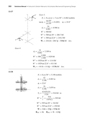
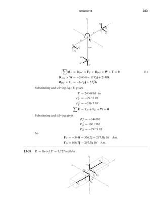
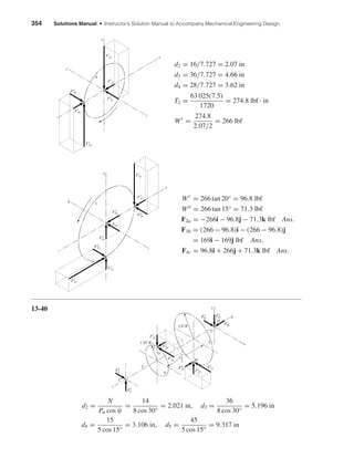
356. 356 Solutions Manual • Instructor’s Solution Manual to Accompany Mechanical Engineering Design
Solving gives
Fx
C = 1987 + 1188 − 1610 = 1565 lbf
F
y
C = 746 − 499 + 425 = 672 lbf
Fz
D = −532 + 686 = 154 lbf Ans.
13-41
VW =
πdW nW
60
=
π(0.100)(600)
60
= π m/s
WWt =
H
VW
=
2000
π
= 637 N
L = px NW = 25(1) = 25 mm
λ = tan−1 L
πdW
= tan−1 25
π(100)
= 4.550° lead angle
W =
WWt
cos φn sin λ + f cos λ
VS =
VW
cos λ
=
π
cos 4.550°
= 3.152 m/s
In ft/min: VS = 3.28(3.152) = 10.33 ft/s = 620 ft/min
Use f = 0.043 from curve A of Fig. 13-42. Then from the first of Eq. (13-43)
W =
637
cos 14.5°(sin 4.55°) + 0.043 cos 4.55°
= 5323 N
W y
= W sin φn = 5323 sin 14.5° = 1333 N
Wz
= 5323[cos 14.5°(cos 4.55°) − 0.043 sin 4.55°] = 5119 N
The force acting against the worm is
W = −637i + 1333j + 5119k N
Thus A is the thrust bearing. Ans.
RAG = −0.05j − 0.10k, RAB = −0.20k
MA = RAG × W + RAB × FB + T = 0
RAG × W = −122.6i + 63.7j − 31.85k
RAB × FB = 0.2F
y
Bi − 0.2Fx
Bj
Substituting and solving gives
T = 31.85 N · m Ans.
Fx
B = 318.5 N, F
y
B = 613 N
So FB = 318.5i + 613j N Ans.
B
G
A x
y
z
Worm shaft diagram
100
100
Wr
Wt
Wa
50
shi20396_ch13.qxd 8/29/03 12:16 PM Page 356

357. Chapter 13 357
Or FB = [(613)2
+ (318.5)2
]1/2
= 691 N radial
F = FA + W + RB = 0
FA = −(W + FB) = −(−637i + 1333j + 5119k + 318.5i + 613j)
= 318.5i − 1946j − 5119k Ans.
Radial Fr
A = 318.5i − 1946j N,
Fr
A = [(318.5)2
+ (−1946)2
]1/2
= 1972 N
Thrust Fa
A = −5119 N
13-42 From Prob. 13-41
WG = 637i − 1333j − 5119k N
pt = px
So dG =
NG px
π
=
48(25)
π
= 382 mm
Bearing D to take thrust load
MD = RDG × WG + RDC × FC + T = 0
RDG = −0.0725i + 0.191j
RDC = −0.1075i
The position vectors are in meters.
RDG × WG = −977.7i − 371.1j − 25.02k
RDC × FC = 0.1075 Fz
Cj − 0.1075F
y
Ck
Putting it together and solving
Gives
T = 977.7 N · m Ans.
FC = −233j + 3450k N, FC = 3460 N Ans.
F = FC + WG + FD = 0
FD = −(FC + WG) = −637i + 1566j + 1669k N Ans.
G
x
y
z
FD
FC
WG
D
C
72.5
191
35
Not to scale
shi20396_ch13.qxd 8/29/03 12:16 PM Page 357

358. 358 Solutions Manual • Instructor’s Solution Manual to Accompany Mechanical Engineering Design
Radial Fr
D = 1566j + 1669k N
Or Fr
D = 2289 N (total radial)
Ft
D = −637i N (thrust)
13-43
VW =
π(1.5)(900)
12
= 353.4 ft/min
Wx
= WWt =
33 000(0.5)
353.4
= 46.69 lbf
pt = px =
π
10
= 0.314 16 in
L = 0.314 16(2) = 0.628 in
λ = tan−1 0.628
π(1.5)
= 7.59°
W =
46.7
cos 14.5° sin 7.59° + 0.05 cos 7.59°
= 263 lbf
W y
= 263 sin 14.5◦
= 65.8 lbf
Wz
= 263[cos 14.5◦
(cos 7.59◦
) − 0.05 sin 7.59◦
] = 251 lbf
So W = 46.7i + 65.8j + 251k lbf Ans.
T = 46.7(0.75) = 35 lbf · in Ans.
13-44
100:101 Mesh
dP =
100
48
= 2.083 33 in
dG =
101
48
= 2.104 17 in
x
y
z
WWt
G
0.75"
T
y
z
shi20396_ch13.qxd 8/29/03 12:16 PM Page 358

359. Chapter 13 359
Proper center-to-center distance:
C =
dP + dG
2
=
2.083 33 + 2.104 17
2
= 2.093 75 in
rbP = r cos φ =
2.0833
2
cos 20◦
= 0.9788 in
99:100 Mesh
dP =
99
48
= 2.0625 in
dG =
100
48
= 2.083 33 in
Proper: C =
99/48 + 100/48
2
= 2.072 917 in
rbP = r cos φ =
2.0625
2
cos 20◦
= 0.969 06 in
Improper: C =
dP + dG
2
=
dP + (100/99)dP
2
= 2.093 75 in
dP =
2(2.093 75)
1 + (100/99)
= 2.0832 in
φ = cos−1 rbP
dP/2
= cos−1 0.969 06
2.0832/2
= 21.5°
From Ex. 13-1 last line
φ = cos−1 rbP
dP/2
= cos−1 (dP/2) cos φ
dP/2
= cos−1 (NP/P) cos φ
(2C /(1 + mG))
= cos−1 (1 + mG)NP cos φ
2PC
Ans.
13-45 Computer programs will vary.
shi20396_ch13.qxd 8/29/03 12:16 PM Page 359

360. Chapter 14
14-1
d =
N
P
=
22
6
= 3.667 in
Table 14-2: Y = 0.331
V =
πdn
12
=
π(3.667)(1200)
12
= 1152 ft/min
Eq. (14-4b): Kv =
1200 + 1152
1200
= 1.96
Wt
=
T
d/2
=
63 025H
nd/2
=
63 025(15)
1200(3.667/2)
= 429.7 lbf
Eq. (14-7):
σ =
KvWt P
FY
=
1.96(429.7)(6)
2(0.331)
= 7633 psi = 7.63 kpsi Ans.
14-2
d =
16
12
= 1.333 in, Y = 0.296
V =
π(1.333)(700)
12
= 244.3 ft/min
Eq. (14-4b): Kv =
1200 + 244.3
1200
= 1.204
Wt
=
63 025H
nd/2
=
63 025(1.5)
700(1.333/2)
= 202.6 lbf
Eq. (14-7):
σ =
KvWt P
FY
=
1.204(202.6)(12)
0.75(0.296)
= 13 185 psi = 13.2 kpsi Ans.
14-3
d = mN = 1.25(18) = 22.5 mm, Y = 0.309
V =
π(22.5)(10−3
)(1800)
60
= 2.121 m/s
Eq. (14-6b): Kv =
6.1 + 2.121
6.1
= 1.348
Wt
=
60H
πdn
=
60(0.5)(103
)
π(22.5)(10−3)(1800)
= 235.8 N
Eq. (14-8): σ =
KvWt
FmY
=
1.348(235.8)
12(1.25)(0.309)
= 68.6 MPa Ans.
shi20396_ch14.qxd 8/20/03 12:43 PM Page 360

361. Chapter 14 361
14-4
d = 5(15) = 75 mm, Y = 0.290
V =
π(75)(10−3
)(200)
60
= 0.7854 m/s
Assume steel and apply Eq. (14-6b):
Kv =
6.1 + 0.7854
6.1
= 1.129
Wt
=
60H
πdn
=
60(5)(103
)
π(75)(10−3)(200)
= 6366 N
Eq. (14-8): σ =
KvWt
FmY
=
1.129(6366)
60(5)(0.290)
= 82.6 MPa Ans.
14-5
d = 1(16) = 16 mm, Y = 0.296
V =
π(16)(10−3
)(400)
60
= 0.335 m/s
Assume steel and apply Eq. (14-6b):
Kv =
6.1 + 0.335
6.1
= 1.055
Wt
=
60H
πdn
=
60(0.15)(103
)
π(16)(10−3)(400)
= 447.6 N
Eq. (14-8): F =
KvWt
σmY
=
1.055(447.6)
150(1)(0.296)
= 10.6 mm
From Table A-17, use F = 11 mm Ans.
14-6
d = 1.5(17) = 25.5 mm, Y = 0.303
V =
π(25.5)(10−3
)(400)
60
= 0.534 m/s
Eq. (14-6b): Kv =
6.1 + 0.534
6.1
= 1.088
Wt
=
60H
πdn
=
60(0.25)(103
)
π(25.5)(10−3)(400)
= 468 N
Eq. (14-8): F =
KvWt
σmY
=
1.088(468)
75(1.5)(0.303)
= 14.9 mm
Use F = 15 mm Ans.
shi20396_ch14.qxd 8/20/03 12:43 PM Page 361

362. 362 Solutions Manual • Instructor’s Solution Manual to Accompany Mechanical Engineering Design
14-7
d =
24
5
= 4.8 in, Y = 0.337
V =
π(4.8)(50)
12
= 62.83 ft/min
Eq. (14-4b): Kv =
1200 + 62.83
1200
= 1.052
Wt
=
63 025H
nd/2
=
63 025(6)
50(4.8/2)
= 3151 lbf
Eq. (14-7): F =
KvWt P
σY
=
1.052(3151)(5)
20(103)(0.337)
= 2.46 in
Use F = 2.5 in Ans.
14-8
d =
16
5
= 3.2 in, Y = 0.296
V =
π(3.2)(600)
12
= 502.7 ft/min
Eq. (14-4b): Kv =
1200 + 502.7
1200
= 1.419
Wt
=
63 025(15)
600(3.2/2)
= 984.8 lbf
Eq. (14-7): F =
KvWt P
σY
=
1.419(984.8)(5)
10(103)(0.296)
= 2.38 in
Use F = 2.5 in Ans.
14-9 Try P = 8 which gives d = 18/8 = 2.25 in and Y = 0.309.
V =
π(2.25)(600)
12
= 353.4 ft/min
Eq. (14-4b): Kv =
1200 + 353.4
1200
= 1.295
Wt
=
63 025(2.5)
600(2.25/2)
= 233.4 lbf
Eq. (14-7): F =
KvWt P
σY
=
1.295(233.4)(8)
10(103)(0.309)
= 0.783 in
shi20396_ch14.qxd 8/20/03 12:43 PM Page 362

363. Chapter 14 363
Using coarse integer pitches from Table 13-2, the following table is formed.
P d V Kv Wt
F
2 9.000 1413.717 2.178 58.356 0.082
3 6.000 942.478 1.785 87.535 0.152
4 4.500 706.858 1.589 116.713 0.240
6 3.000 471.239 1.393 175.069 0.473
8 2.250 353.429 1.295 233.426 0.782
10 1.800 282.743 1.236 291.782 1.167
12 1.500 235.619 1.196 350.139 1.627
16 1.125 176.715 1.147 466.852 2.773
Other considerations may dictate the selection. Good candidates are P = 8 (F = 7/8 in)
and P = 10 (F = 1.25 in). Ans.
14-10 Try m = 2 mm which gives d = 2(18) = 36 mm and Y = 0.309.
V =
π(36)(10−3
)(900)
60
= 1.696 m/s
Eq. (14-6b): Kv =
6.1 + 1.696
6.1
= 1.278
Wt
=
60(1.5)(103
)
π(36)(10−3)(900)
= 884 N
Eq. (14-8): F =
1.278(884)
75(2)(0.309)
= 24.4 mm
Using the preferred module sizes from Table 13-2:
m d V Kv Wt
F
1.00 18.0 0.848 1.139 1768.388 86.917
1.25 22.5 1.060 1.174 1414.711 57.324
1.50 27.0 1.272 1.209 1178.926 40.987
2.00 36.0 1.696 1.278 884.194 24.382
3.00 54.0 2.545 1.417 589.463 12.015
4.00 72.0 3.393 1.556 442.097 7.422
5.00 90.0 4.241 1.695 353.678 5.174
6.00 108.0 5.089 1.834 294.731 3.888
8.00 144.0 6.786 2.112 221.049 2.519
10.00 180.0 8.482 2.391 176.839 1.824
12.00 216.0 10.179 2.669 147.366 1.414
16.00 288.0 13.572 3.225 110.524 0.961
20.00 360.0 16.965 3.781 88.419 0.721
25.00 450.0 21.206 4.476 70.736 0.547
32.00 576.0 27.143 5.450 55.262 0.406
40.00 720.0 33.929 6.562 44.210 0.313
50.00 900.0 42.412 7.953 35.368 0.243
Other design considerations may dictate the size selection. For the present design,
m = 2 mm (F = 25 mm) is a good selection. Ans.
shi20396_ch14.qxd 8/20/03 12:43 PM Page 363

364. 364 Solutions Manual • Instructor’s Solution Manual to Accompany Mechanical Engineering Design
14-11
dP =
22
6
= 3.667 in, dG =
60
6
= 10 in
V =
π(3.667)(1200)
12
= 1152 ft/min
Eq. (14-4b): Kv =
1200 + 1152
1200
= 1.96
Wt
=
63 025(15)
1200(3.667/2)
= 429.7 lbf
Table 14-8: Cp = 2100 psi
Eq. (14-12): r1 =
3.667 sin 20°
2
= 0.627 in, r2 =
10 sin 20°
2
= 1.710 in
Eq. (14-14): σC = −Cp
KvWt
F cos φ
1
r1
+
1
r2
1/2
= −2100
1.96(429.7)
2 cos 20°
1
0.627
+
1
1.710
1/2
= −65.6(103
) psi = −65.6 kpsi Ans.
14-12
dP =
16
12
= 1.333 in, dG =
48
12
= 4 in
V =
π(1.333)(700)
12
= 244.3 ft/min
Eq. (14-4b): Kv =
1200 + 244.3
1200
= 1.204
Wt
=
63 025(1.5)
700(1.333/2)
= 202.6 lbf
Table 14-8: Cp = 2100
√
psi
Eq. (14-12): r1 =
1.333 sin 20°
2
= 0.228 in, r2 =
4 sin 20°
2
= 0.684 in
Eq. (14-14):
σC = −2100
1.202(202.6)
F cos 20°
1
0.228
+
1
0.684
1/2
= −100(103
)
F =
2100
100(103)
2
1.202(202.6)
cos 20°
1
0.228
+
1
0.684
= 0.668 in
Use F = 0.75 in Ans.
shi20396_ch14.qxd 8/20/03 12:43 PM Page 364

365. Chapter 14 365
14-13
dP =
24
5
= 4.8 in, dG =
48
5
= 9.6 in
Eq. (14-4a):
V =
π(4.8)(50)
12
= 62.83 ft/min
Kv =
600 + 62.83
600
= 1.105
Wt
=
63 025H
50(4.8/2)
= 525.2H
Table 14-8: Cp = 1960
√
psi
Eq. (14-12): r1 =
4.8 sin 20◦
2
= 0.821 in, r2 = 2r1 = 1.642 in
Eq. (14-14): −100(103
) = −1960
1.105(525.2H)
2.5 cos 20◦
1
0.821
+
1
1.642
1/2
H = 5.77 hp Ans.
14-14
dP = 4(20) = 80 mm, dG = 4(32) = 128 mm
V =
π(80)(10−3
)(1000)
60
= 4.189 m/s
Kv =
3.05 + 4.189
3.05
= 2.373
Wt
=
60(10)(103
)
π(80)(10−3)(1000)
= 2387 N
Cp = 163
√
MPa
r1 =
80 sin 20°
2
= 13.68 mm, r2 =
128 sin 20°
2
= 21.89 mm
σC = −163
2.373(2387)
50 cos 20°
1
13.68
+
1
21.89
1/2
= −617 MPa Ans.
14-15 The pinion controls the design.
Bending YP = 0.303, YG = 0.359
dP =
17
12
= 1.417 in, dG =
30
12
= 2.500 in
V =
πdPn
12
=
π(1.417)(525)
12
= 194.8 ft/min
Eq. (14-4b): Kv =
1200 + 194.8
1200
= 1.162
Eq. (7-8): Se = 0.504(76) = 38 300 psi
Eq. (7-18): ka = 2.70(76)−0.265
= 0.857
Eq. (14-6a):
Table 14-8:
Eq. (14-12):
Eq. (14-14):
shi20396_ch14.qxd 8/20/03 12:43 PM Page 365

366. 366 Solutions Manual • Instructor’s Solution Manual to Accompany Mechanical Engineering Design
l =
2.25
Pd
=
2.25
12
= 0.1875 in
x =
3YP
2P
=
3(0.303)
2(12)
= 0.0379 in
t = 4(0.1875)(0.0379) = 0.1686 in
de = 0.808 0.875(0.1686) = 0.310 in
kb =
0.310
0.30
−0.107
= 0.996
kc = kd = ke = 1, kf1
= 1.65
rf =
0.300
12
= 0.025 in
r
d
=
rf
t
=
0.025
0.1686
= 0.148
Approximate D/d = ∞ with D/d = 3; from Fig. A-15-6, Kt = 1.68.
Eq. (7-35): Kf =
1.68
1 +
2
√
0.025
1.68 − 1
1.68
4
76
= 1.323
Miscellaneous-Effects Factor:
kf = kf 1kf 2 = 1.65
1
1.323
= 1.247
Se = 0.857(0.996)(1)(1)(1)(1.247)(38 300)
= 40 770 psi
σall =
40 770
2.25
= 18 120 psi
Wt
=
FYPσall
Kv Pd
=
0.875(0.303)(18 120)
1.162(12)
= 345 lbf
H =
345(194.8)
33 000
= 2.04 hp Ans.
Wear
ν1 = ν2 = 0.292, E1 = E2 = 30(106
) psi
Eq. (14-14): Cp = 2300 psi
r1 =
dP
2
sin φ =
1.417
2
sin 20° = 0.242 in
r2 =
dG
2
sin φ =
2.500
2
sin 20° = 0.428
1
r1
+
1
r2
=
1
0.242
+
1
0.428
= 6.469 in−1
Eq. (14-12):
Eq. (7-17):
Eq. (14-3):
Eq. (7-24):
Eq. (7-19):
shi20396_ch14.qxd 8/20/03 12:43 PM Page 366

367. Chapter 14 367
From Eq. (7-68),
(SC)108 = 0.4HB − 10 kpsi
= [0.4(149) − 10](103
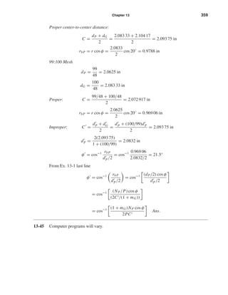
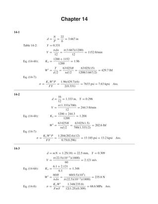
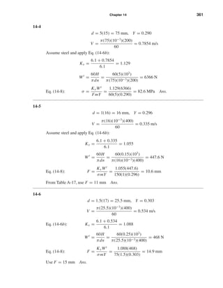
) = 49 600 psi
σC,all =
−49 600
√
2.25
= −33 067 psi
Wt
=
−33 067
2300
2
0.875 cos 20°
1.162(6.469)
= 22.6 lbf
H =
22.6(194.8)
33 000
= 0.133 hp Ans.
Rating power (pinion controls):
H1 = 2.04 hp
H2 = 0.133 hp
Hall = (min 2.04, 0.133) = 0.133 hp Ans.
14-16 Pinion controls: YP = 0.322, YG = 0.447
Bending dP = 20/3 = 6.667 in, dG = 33.333 in
V = πdPn/12 = π(6.667)(870)/12 = 1519 ft/min
Kv = (1200 + 1519)/1200 = 2.266
Se = 0.504(113) = 56.950 kpsi = 56 950 psi
ka = 2.70(113)−0.265
= 0.771
l = 2.25/Pd = 2.25/3 = 0.75 in
x = 3(0.322)/[2(3)] = 0.161 in
t = 4(0.75)(0.161) = 0.695 in
de = 0.808 2.5(0.695) = 1.065 in
kb = (1.065/0.30)−0.107
= 0.873
kc = kd = ke = 1
rf = 0.300/3 = 0.100 in
r
d
=
rf
t
=
0.100
0.695
= 0.144
From Table A-15-6, Kt = 1.75; Eq. (7-35): Kf = 1.597
kf 2 = 1/1.597, kf = kf 1kf 2 = 1.65/1.597 = 1.033
Se = 0.771(0.873)(1)(1)(1)(1.033)(56 950) = 39 600 psi
σall = 39 600/1.5 = 26 400 psi
Wt
=
FYPσall
Kv Pd
=
2.5(0.322)(26 400)
2.266(3)
= 3126 lbf
H = Wt
V/33 000 = 3126(1519)/33 000 = 144 hp Ans.
shi20396_ch14.qxd 8/20/03 12:43 PM Page 367

368. 368 Solutions Manual • Instructor’s Solution Manual to Accompany Mechanical Engineering Design
Wear
Cp = 2300 psi
r1 = (6.667/2) sin 20° = 1.140 in
r2 = (33.333/2) sin 20° = 5.700 in
SC = [0.4(262) − 10](103
) = 94 800 psi
σC,all = −SC/
√
nd = −94.800/
√
1.5 = −77 404 psi
Wt
=
σC,all
Cp
2
F cos φ
Kv
1
1/r1 + 1/r2
=
−77 404
2300
2
2.5 cos 20°
2.266
1
1/1.140 + 1/5.700
= 1115 lbf
H =
Wt V
33 000
=
1115(1519)
33 000
= 51.3 hp Ans.
For 108
cycles (revolutions of the pinion), the power based on wear is 51.3 hp.
Rating power–pinion controls
H1 = 144 hp
H2 = 51.3 hp
Hrated = min(144, 51.3) = 51.3 hp Ans.
14-17 Given: φ = 20°, n = 1145 rev/min, m = 6 mm, F = 75 mm, NP = 16 milled teeth,
NG = 30T, Sut = 900 MPa, HB = 260, nd = 3, YP = 0.296, and YG = 0.359.
Pinion bending
dP = mNP = 6(16) = 96 mm
dG = 6(30) = 180 mm
V =
πdPn
12
=
π(96)(1145)(10−3
)(12)
(12)(60)
= 5.76 m/s
Eq. (14-6b): Kv =
6.1 + 5.76
6.1
= 1.944
Se = 0.504(900) = 453.6 MPa
a = 4.45, b = −0.265
ka = 4.51(900)−0.265
= 0.744
l = 2.25m = 2.25(6) = 13.5 mm
x = 3Ym/2 = 3(0.296)6/2 = 2.664 mm
t =
√
4lx = 4(13.5)(2.664) = 12.0 mm
de = 0.808 75(12.0) = 24.23 mm
Table 14-8:
Eq. (14-12):
Eq. (7-68):
shi20396_ch14.qxd 8/20/03 12:43 PM Page 368

369. Chapter 14 369
kb =
24.23
7.62
−0.107
= 0.884
kc = kd = ke = 1
rf = 0.300m = 0.300(6) = 1.8 mm
From Fig. A-15-6 for r/d = rf /t = 1.8/12 = 0.15, Kt = 1.68.
Kf =
1.68
1 + 2
√
1.8 [(1.68 − 1)/1.68](139/900)
= 1.537
kf 1 = 1.65 (Gerber failure criterion)
kf 2 = 1/Kf = 1/1.537 = 0.651
kf = kf 1kf 2 = 1.65(0.651) = 1.074
Se = 0.744(0.884)(1)(1)(1)(1.074)(453.6) = 320.4 MPa
σall =
Se
nd
=
320.4
1.3
= 246.5 MPa
Eq. (14-8): Wt
=
FYmσall
Kv
=
75(0.296)(6)(246.5)
1.944
= 16 890 N
H =
Tn
9.55
=
16 890(96/2)(1145)
9.55(106)
= 97.2 kW Ans.
Wear: Pinion and gear
Eq. (14-12): r1 = (96/2) sin 20◦
= 16.42 mm
r2 = (180/2) sin 20◦
= 30.78 mm
Table 14-8: Cp ˙= 191
√
MPa
Eq. (7-68): SC = 6.89[0.4(260) − 10] = 647.7 MPa
σC,all = −
647.7
√
1.3
= −568 MPa
Eq. (14-14): Wt
=
σC,all
Cp
2
F cos φ
Kv
1
1/r1 + 1/r2
=
−568
191
2
75 cos 20◦
1.944
1
1/16.42 + 1/30.78
= 3433 N
T =
WtdP
2
=
3433(96)
2
= 164 784 N · mm = 164.8 N · m
H =
Tn
9.55
=
164.8(1145)
9.55
= 19 758.7 W = 19.8 kW Ans.
Thus, wear controls the gearset power rating; H = 19.8 kW. Ans.
shi20396_ch14.qxd 8/20/03 12:43 PM Page 369

370. 370 Solutions Manual • Instructor’s Solution Manual to Accompany Mechanical Engineering Design
14-18 Preliminaries: NP = 17, NG = 51
dP =
N
Pd
=
17
6
= 2.833 in
dG =
51
6
= 8.500 in
V = πdPn/12 = π(2.833)(1120)/12 = 830.7 ft/min
Eq. (14-4b): Kv = (1200 + 830.7)/1200 = 1.692
σall =
Sy
nd
=
90 000
2
= 45 000 psi
Table 14-2: YP = 0.303, YG = 0.410
Eq. (14-7): Wt
=
FYPσall
Kv Pd
=
2(0.303)(45 000)
1.692(6)
= 2686 lbf
H =
WtV
33 000
=
2686(830.7)
33 000
= 67.6 hp
Based on yielding in bending, the power is 67.6 hp.
(a) Pinion fatigue
Bending
Se = 0.504(232/2) = 58 464 psi
a = 2.70, b = −0.265, ka = 2.70(116)−0.265
= 0.766
Table 13-1: l =
1
Pd
+
1.25
Pd
=
2.25
Pd
=
2.25
6
= 0.375 in
Eq. (14-3): x =
3YP
2Pd
=
3(0.303)
2(6)
= 0.0758
t =
√
4lx = 4(0.375)(0.0758) = 0.337 in
de = 0.808
√
Ft = 0.808 2(0.337) = 0.663 in
kb =
0.663
0.30
−0.107
= 0.919
kc = kd = ke = 1. Assess two components contributing to kf . First, based upon
one-way bending and the Gerber failure criterion, kf 1 = 1.65. Second, due to stress-
concentration,
rf =
0.300
Pd
=
0.300
6
= 0.050 in
Fig. A-15-6:
r
d
=
rf
t
=
0.05
0.338
= 0.148
shi20396_ch14.qxd 8/20/03 12:43 PM Page 370

371. Chapter 14 371
Estimate D/d = ∞ by setting D/d = 3, Kt = 1.68. From Eq. (7-35) and Table 7-8,
Kf =
1.68
1 + 2
√
0.05 [(1.68 − 1)/1.68](4/116)
= 1.494
kf 2 =
1
Kf
=
1
1.494
= 0.669
kf = kf 1kf 2 = 1.65(0.669) = 1.104
Se = 0.766(0.919)(1)(1)(1)(1.104)(58 464) = 45 436 psi
σall =
Se
nd
=
45 436
2
= 22 718 psi
Wt
=
FYPσall
Kv Pd
=
2(0.303)(22 718)
1.692(6)
= 1356 lbf
H =
Wt V
33 000
=
1356(830.7)
33 000
= 34.1 hp Ans.
(b) Pinion fatigue
Wear
From Table A-5 for steel: ν = 0.292, E = 30(106
) psi
Eq. (14-13) or Table 14-8:
Cp =
1
2π[(1 − 0.2922)/30(106)]
1/2
= 2285 psi
In preparation for Eq. (14-14):
Eq. (14-12): r1 =
dP
2
sin φ =
2.833
2
sin 20◦
= 0.485 in
r2 =
dG
2
sin φ =
8.500
2
sin 20◦
= 1.454 in
1
r1
+
1
r2
=
1
0.485
+
1
1.454
= 2.750 in
Eq. (7-68): (SC)108 = 0.4HB − 10 kpsi
In terms of gear notation
σC = [0.4(232) − 10]103
= 82 800 psi
We will introduce the design factor of nd = 2 and apply it to the load Wt
by dividing
by
√
2.
σC,all = −
σc
√
2
= −
82 800
√
2
= −58 548 psi
shi20396_ch14.qxd 8/20/03 12:43 PM Page 371

372. 372 Solutions Manual • Instructor’s Solution Manual to Accompany Mechanical Engineering Design
Solve Eq. (14-14) for Wt
:
Wt
=
−58 548
2285
2
2 cos 20◦
1.692(2.750)
= 265 lbf
Hall =
265(830.7)
33 000
= 6.67 hp Ans.
For 108
cycles (turns of pinion), the allowable power is 6.67 hp.
(c) Gear fatigue due to bending and wear
Bending
Eq. (14-3): x =
3YG
2Pd
=
3(0.4103)
2(6)
= 0.1026 in
t = 4(0.375)(0.1026) = 0.392 in
de = 0.808 2(0.392) = 0.715 in
kb =
0.715
0.30
−0.107
= 0.911
kc = kd = ke = 1
r
d
=
rf
t
=
0.050
0.392
= 0.128
Approximate D/d = ∞ by setting D/d = 3 for Fig. A-15-6; Kt = 1.80. Use Kf =
1.583.
kf 2 =
1
1.583
= 0.632, kf = 1.65(0.632) = 1.043
Se = 0.766(0.911)(1)(1)(1)(1.043)(58 464) = 42 550 psi
σall =
Se
2
=
42 550
2
= 21 275 psi
Wt
=
2(0.4103)(21 275)
1.692(6)
= 1720 lbf
Hall =
1720(830.7)
33 000
= 43.3 hp Ans.
The gear is thus stronger than the pinion in bending.
Wear Since the material of the pinion and the gear are the same, and the contact
stresses are the same, the allowable power transmission of both is the same. Thus,
Hall = 6.67 hp for 108
revolutions of each. As yet, we have no way to establish SC for
108
/3 revolutions.
shi20396_ch14.qxd 8/20/03 12:43 PM Page 372

373. Chapter 14 373
(d) Pinion bending: H1 = 34.1 hp
Pinion wear: H2 = 6.67 hp
Gear bending: H3 = 43.3 hp
Gear wear: H4 = 6.67 hp
Power rating of the gear set is thus
Hrated = min(34.1, 6.67, 43.3, 6.67) = 6.67 hp Ans.
14-19 dP = 16/6 = 2.667 in, dG = 48/6 = 8 in
V =
π(2.667)(300)
12
= 209.4 ft/min
Wt
=
33 000(5)
209.4
= 787.8 lbf
Assuming uniform loading, Ko = 1. From Eq. (14-28),
Qv = 6, B = 0.25(12 − 6)2/3
= 0.8255
A = 50 + 56(1 − 0.8255) = 59.77
Eq. (14-27):
Kv =
59.77 +
√
209.4
59.77
0.8255
= 1.196
From Table 14-2,
NP = 16T, YP = 0.296
NG = 48T, YG = 0.4056
From Eq. (a), Sec. 14-10 with F = 2 in
(Ks)P = 1.192
2
√
0.296
6
0.0535
= 1.088
(Ks)G = 1.192
2
√
0.4056
6
0.0535
= 1.097
From Eq. (14-30) with Cmc = 1
Cpf =
2
10(2.667)
− 0.0375 + 0.0125(2) = 0.0625
Cpm = 1, Cma = 0.093 (Fig. 14-11), Ce = 1
Km = 1 + 1[0.0625(1) + 0.093(1)] = 1.156
Assuming constant thickness of the gears → KB = 1
mG = NG/NP = 48/16 = 3
With N (pinion) = 108
cycles and N (gear) = 108
/3, Fig. 14-14 provides the relations:
(YN )P = 1.3558(108
)−0.0178
= 0.977
(YN )G = 1.3558(108
/3)−0.0178
= 0.996
shi20396_ch14.qxd 8/20/03 12:43 PM Page 373

374. 374 Solutions Manual • Instructor’s Solution Manual to Accompany Mechanical Engineering Design
Fig. 14-6: JP = 0.27, JG ˙= 0.38
From Table 14-10 for R = 0.9, KR = 0.85
KT = Cf = 1
Eq. (14-23) with mN = 1 I =
cos 20◦ sin 20◦
2
3
3 + 1
= 0.1205
Table 14-8: Cp = 2300 psi
Strength: Grade 1 steel with HBP = HBG = 200
Fig. 14-2: (St)P = (St)G = 77.3(200) + 12 800 = 28 260 psi
Fig. 14-5: (Sc)P = (Sc)G = 322(200) + 29 100 = 93 500 psi
Fig. 14-15: (ZN )P = 1.4488(108
)−0.023
= 0.948
(ZN )G = 1.4488(108
/3)−0.023
= 0.973
Sec. 14-12: HBP/HBG = 1 ∴ CH = 1
Pinion tooth bending
Eq. (14-15):
(σ)P = Wt
KoKv Ks
Pd
F
Km KB
J
= 787.8(1)(1.196)(1.088)
6
2
(1.156)(1)
0.27
= 13 167 psi Ans.
Factor of safety from Eq. (14-41)
(SF)P =
StYN /(KT KR)
σ
=
28 260(0.977)/[(1)(0.85)]
13 167
= 2.47 Ans.
Gear tooth bending
(σ)G = 787.8(1)(1.196)(1.097)
6
2
(1.156)(1)
0.38
= 9433 psi Ans.
(SF)G =
28 260(0.996)/[(1)(0.85)]
9433
= 3.51 Ans.
Pinion tooth wear
Eq. (14-16): (σc)P = Cp Wt
KoKv Ks
Km
dP F
Cf
I
1/2
P
= 2300 787.8(1)(1.196)(1.088)
1.156
2.667(2)
1
0.1205
1/2
= 98 760 psi Ans.
Eq. (14-42):
(SH )P =
Sc ZN /(KT KR)
σc P
=
93 500(0.948)/[(1)(0.85)]
98 760
= 1.06 Ans.
shi20396_ch14.qxd 8/20/03 12:43 PM Page 374

375. Chapter 14 375
Gear tooth wear
(σc)G =
(Ks)G
(Ks)P
1/2
(σc)P =
1.097
1.088
1/2
(98 760) = 99 170 psi Ans.
(SH )G =
93 500(0.973)(1)/[(1)(0.85)]
99 170
= 1.08 Ans.
The hardness of the pinion and the gear should be increased.
14-20 dP = 2.5(20) = 50 mm, dG = 2.5(36) = 90 mm
V =
πdPnP
60
=
π(50)(10−3
)(100)
60
= 0.2618 m/s
Wt
=
60(120)
π(50)(10−3)(100)
= 458.4 N
Eq. (14-28): Ko = 1, Qv = 6, B = 0.25(12 − 6)2/3
= 0.8255
A = 50 + 56(1 − 0.8255) = 59.77
Eq. (14-27): Kv =
59.77 +
√
200(0.2618)
59.77
0.8255
= 1.099
Table 14-2: YP = 0.322, YG = 0.3775
Similar to Eq. (a) of Sec. 14-10 but for SI units:
Ks =
1
kb
= 0.8433 mF
√
Y
0.0535
(Ks)P = 0.8433 2.5(18)
√
0.322
0.0535
= 1.003 use 1
(Ks)G = 0.8433 2.5(18)
√
0.3775
0.0535
> 1 use 1
Cmc = 1, F = 18/25.4 = 0.709 in, Cpf =
18
10(50)
− 0.025 = 0.011
Cpm = 1, Cma = 0.247 + 0.0167(0.709) − 0.765(10−4
)(0.7092
) = 0.259
Ce = 1
KH = 1 + 1[0.011(1) + 0.259(1)] = 1.27
Eq. (14-40): KB = 1, mG = NG/NP = 36/20 = 1.8
Fig. 14-14: (YN )P = 1.3558(108
)−0.0178
= 0.977
(YN )G = 1.3558(108
/1.8)−0.0178
= 0.987
Fig. 14-6: (YJ )P = 0.33, (YJ )G = 0.38
Eq. (14-38): YZ = 0.658 − 0.0759 ln(1 − 0.95) = 0.885
Yθ = ZR = 1
shi20396_ch14.qxd 8/20/03 12:43 PM Page 375

376. 376 Solutions Manual • Instructor’s Solution Manual to Accompany Mechanical Engineering Design
Eq. (14-23) with mN = 1:
ZI =
cos 20◦ sin 20◦
2
1.8
1.8 + 1
= 0.103
Table 14-8: ZE = 191
√
MPa
Strength Grade 1 steel, HBP = HBG = 200
Fig. 14-2: (σF P)P = (σF P)G = 0.533(200) + 88.3 = 194.9 MPa
Fig. 14-5: (σH P)P = (σH P)G = 2.22(200) + 200 = 644 MPa
Fig. 14-15: (ZN )P = 1.4488(108
)−0.023
= 0.948
(ZN )G = 1.4488(108
/1.8)−0.023
= 0.961
HBP/HBG = 1 ∴ ZW = 1
Pinion tooth bending
(σ)P = Wt
KoKv Ks
1
bmt
KH KB
YJ P
= 458.4(1)(1.099)(1)
1
18(2.5)
1.27(1)
0.33
= 43.08 MPa Ans.
(SF)P =
σF P
σ
YN
Yθ YZ P
=
194.9
43.08
0.977
1(0.885)
= 4.99 Ans.
Gear tooth bending
(σ)G = 458.4(1)(1.099)(1)
1
18(2.5)
1.27(1)
0.38
= 37.42 MPa Ans.
(SF)G =
194.9
37.42
0.987
1(0.885)
= 5.81 Ans.
Pinion tooth wear
(σc)P = ZE Wt KoKv Ks
KH
dw1b
ZR
ZI
P
= 191 458.4(1)(1.099)(1)
1.27
50(18)
1
0.103
= 501.8 MPa Ans.
(SH )P =
σH P
σc
ZN ZW
Yθ YZ P
=
644
501.8
0.948(1)
1(0.885)
= 1.37 Ans.
Gear tooth wear
(σc)G =
(Ks)G
(Ks)P
1/2
(σc)P =
1
1
1/2
(501.8) = 501.8 MPa Ans.
(SH )G =
644
501.8
0.961(1)
1(0.885)
= 1.39 Ans.
shi20396_ch14.qxd 8/20/03 12:43 PM Page 376

377. Chapter 14 377
14-21
Pt = Pn cos ψ = 6 cos 30° = 5.196 teeth/in
dP =
16
5.196
= 3.079 in, dG =
48
16
(3.079) = 9.238 in
V =
π(3.079)(300)
12
= 241.8 ft/min
Wt
=
33 000(5)
241.8
= 682.3 lbf, Kv =
59.77 +
√
241.8
59.77
0.8255
= 1.210
From Prob. 14-19:
YP = 0.296, YG = 0.4056
(Ks)P = 1.088, (Ks)G = 1.097, KB = 1
mG = 3, (YN )P = 0.977, (YN )G = 0.996, KR = 0.85
(St)P = (St)G = 28 260 psi, CH = 1, (Sc)P = (Sc)G = 93 500 psi
(ZN )P = 0.948, (ZN )G = 0.973, Cp = 2300
√
psi
The pressure angle is:
φt = tan−1 tan 20°
cos 30°
= 22.80°
(rb)P =
3.079
2
cos 22.8° = 1.419 in, (rb)G = 3(rb)P = 4.258 in
a = 1/Pn = 1/6 = 0.167 in
Eq. (14-26):
Z =
3.079
2
+ 0.167
2
− 1.4192
1/2
+
9.238
2
+ 0.167
2
− 4.2582
1/2
−
3.079
2
+
9.238
2
sin 22.8°
= 0.9479 + 2.1852 − 2.3865 = 0.7466 Conditions O.K. for use
pN = pn cos φn =
π
6
cos 20° = 0.4920 in
Eq. (14-23): mN =
pN
0.95Z
=
0.492
0.95(0.7466)
= 0.6937
Eq. (14-23): I =
sin 22.8° cos 22.8°
2(0.6937)
3
3 + 1
= 0.193
Fig. 14-7: JP ˙= 0.45, JG ˙= 0.54
shi20396_ch14.qxd 8/20/03 12:43 PM Page 377

378. 378 Solutions Manual • Instructor’s Solution Manual to Accompany Mechanical Engineering Design
Fig. 14-8: Corrections are 0.94 and 0.98
JP = 0.45(0.94) = 0.423, JG = 0.54(0.98) = 0.529
Cmc = 1, Cpf =
2
10(3.079)
− 0.0375 + 0.0125(2) = 0.0525
Cpm = 1, Cma = 0.093, Ce = 1
Km = 1 + (1)[0.0525(1) + 0.093(1)] = 1.146
Pinion tooth bending
(σ)P = 682.3(1)(1.21)(1.088)
5.196
2
1.146(1)
0.423
= 6323 psi Ans.
(SF)P =
28 260(0.977)/[1(0.85)]
6323
= 5.14 Ans.
Gear tooth bending
(σ)G = 682.3(1)(1.21)(1.097)
5.196
2
1.146(1)
0.529
= 5097 psi Ans.
(SF)G =
28 260(0.996)/[1(0.85)]
5097
= 6.50 Ans.
Pinion tooth wear
(σc)P = 2300 682.3(1)(1.21)(1.088)
1.146
3.078(2)
1
0.193
1/2
= 67 700 psi Ans.
(SH )P =
93 500(0.948)/[(1)(0.85)]
67 700
= 1.54 Ans.
Gear tooth wear
(σc)G =
1.097
1.088
1/2
(67 700) = 67 980 psi Ans.
(SH )G =
93 500(0.973)/[(1)(0.85)]
67 980
= 1.57 Ans.
14-22 Given: R = 0.99 at 108
cycles, HB = 232 through-hardening Grade 1, core and case, both
gears. NP = 17T, NG = 51T, YP = 0.303, YG = 0.4103, JP = 0.292, JG = 0.396,
dP = 2.833 in, dG = 8.500 in.
Pinion bending
From Fig. 14-2:
0.99(St)107 = 77.3HB + 12 800
= 77.3(232) + 12 800 = 30 734 psi
shi20396_ch14.qxd 8/20/03 12:43 PM Page 378

379. Chapter 14 379
Fig. 14-14: YN = 1.6831(108
)−0.0323
= 0.928
V = πdPn/12 = π(2.833)(1120/12) = 830.7 ft/min
KT = KR = 1, SF = 2, SH =
√
2
σall =
30 734(0.928)
2(1)(1)
= 14 261 psi
Qv = 5, B = 0.25(12 − 5)2/3
= 0.9148
A = 50 + 56(1 − 0.9148) = 54.77
Kv =
54.77 +
√
830.7
54.77
0.9148
= 1.472
Ks = 1.192
2
√
0.303
6
0.0535
= 1.089 ⇒ use 1
Km = Cm f = 1 + Cmc(Cpf Cpm + CmaCe)
Cmc = 1
Cpf =
F
10d
− 0.0375 + 0.0125F
=
2
10(2.833)
− 0.0375 + 0.0125(2)
= 0.0581
Cpm = 1
Cma = 0.127 + 0.0158(2) − 0.093(10−4
)(22
) = 0.1586
Ce = 1
Km = 1 + 1[0.0581(1) + 0.1586(1)] = 1.2167
Eq. (14-15):
Kβ = 1
Wt
=
F JPσall
KoKv Ks Pd Km Kβ
=
2(0.292)(14 261)
1(1.472)(1)(6)(1.2167)(1)
= 775 lbf
H =
Wt V
33 000
=
775(830.7)
33 000
= 19.5 hp
Pinion wear
Fig. 14-15: ZN = 2.466N−0.056
= 2.466(108
)−0.056
= 0.879
MG = 51/17 = 3
I =
sin 20◦ cos 20◦
2
3
3 + 1
= 1.205, CH = 1
shi20396_ch14.qxd 8/20/03 12:43 PM Page 379

380. 380 Solutions Manual • Instructor’s Solution Manual to Accompany Mechanical Engineering Design
Fig. 14-5: 0.99(Sc)107 = 322HB + 29 100
= 322(232) + 29 100 = 103 804 psi
σc,all =
103 804(0.879)
√
2(1)(1)
= 64 519 psi
Eq. (14-16): Wt
=
σc,all
Cp
2
FdP I
KoKv Ks KmCf
=
64 519
2300
2
2(2.833)(0.1205)
1(1.472)(1)(1.2167)(1)
= 300 lbf
H =
Wt V
33 000
=
300(830.7)
33 000
= 7.55 hp
The pinion controls therefore Hrated = 7.55 hp Ans.
4-23
l = 2.25/Pd, x =
3Y
2Pd
t =
√
4lx = 4
2.25
Pd
3Y
2Pd
=
3.674
Pd
√
Y
de = 0.808
√
Ft = 0.808 F
3.674
Pd
√
Y = 1.5487
F
√
Y
Pd
kb =


1.5487 F
√
Y/Pd
0.30


−0.107
= 0.8389
F
√
Y
Pd
−0.0535
Ks =
1
kb
= 1.192
F
√
Y
Pd
0.0535
Ans.
14-24 YP = 0.331, YG = 0.422, JP = 0.345, JG = 0.410, Ko = 1.25. The service conditions
are adequately described by Ko. Set SF = SH = 1.
dP = 22/4 = 5.500 in
dG = 60/4 = 15.000 in
V =
π(5.5)(1145)
12
= 1649 ft/min
Pinion bending
0.99(St)107 = 77.3HB + 12 800 = 77.3(250) + 12 800 = 32 125 psi
YN = 1.6831[3(109
)]−0.0323
= 0.832
shi20396_ch14.qxd 8/20/03 12:43 PM Page 380

381. Chapter 14 381
Eq. (14-17): (σall)P =
32 125(0.832)
1(1)(1)
= 26 728 psi
B = 0.25(12 − 6)2/3
= 0.8255
A = 50 + 56(1 − 0.8255) = 59.77
Kv =
59.77 +
√
1649
59.77
0.8255
= 1.534
Ks = 1, Cm = 1
Cmc =
F
10d
− 0.0375 + 0.0125F
=
3.25
10(5.5)
− 0.0375 + 0.0125(3.25) = 0.0622
Cma = 0.127 + 0.0158(3.25) − 0.093(10−4
)(3.252
) = 0.178
Ce = 1
Km = Cm f = 1 + (1)[0.0622(1) + 0.178(1)] = 1.240
Kβ = 1, KT = 1
Eq. (14-15): Wt
1 =
26 728(3.25)(0.345)
1.25(1.534)(1)(4)(1.240)
= 3151 lbf
H1 =
3151(1649)
33 000
= 157.5 hp
Gear bending By similar reasoning, Wt
2 = 3861 lbf and H2 = 192.9 hp
Pinion wear
mG = 60/22 = 2.727
I =
cos 20◦ sin 20◦
2
2.727
1 + 2.727
= 0.1176
0.99(Sc)107 = 322(250) + 29 100 = 109 600 psi
(ZN )P = 2.466[3(109
)]−0.056
= 0.727
(ZN )G = 2.466[3(109
)/2.727]−0.056
= 0.769
(σc,all)P =
109 600(0.727)
1(1)(1)
= 79 679 psi
Wt
3 =
σc,all
Cp
2
FdP I
KoKv Ks KmCf
=
79 679
2300
2
3.25(5.5)(0.1176)
1.25(1.534)(1)(1.24)(1)
= 1061 lbf
H3 =
1061(1649)
33 000
= 53.0 hp
shi20396_ch14.qxd 8/20/03 12:43 PM Page 381

382. 382 Solutions Manual • Instructor’s Solution Manual to Accompany Mechanical Engineering Design
Gear wear
Similarly, Wt
4 = 1182 lbf, H4 = 59.0 hp
Rating
Hrated = min(H1, H2, H3, H4)
= min(157.5, 192.9, 53, 59) = 53 hp Ans.
Note differing capacities. Can these be equalized?
14-25 From Prob. 14-24:
Wt
1 = 3151 lbf, Wt
2 = 3861 lbf,
Wt
3 = 1061 lbf, Wt
4 = 1182 lbf
Wt
=
33 000Ko H
V
=
33 000(1.25)(40)
1649
= 1000 lbf
Pinion bending: The factor of safety, based on load and stress, is
(SF)P =
Wt
1
1000
=
3151
1000
= 3.15
Gear bending based on load and stress
(SF)G =
Wt
2
1000
=
3861
1000
= 3.86
Pinion wear
based on load: n3 =
Wt
3
1000
=
1061
1000
= 1.06
based on stress: (SH )P =
√
1.06 = 1.03
Gear wear
based on load: n4 =
Wt
4
1000
=
1182
1000
= 1.18
based on stress: (SH )G =
√
1.18 = 1.09
Factors of safety are used to assess the relative threat of loss of function 3.15, 3.86, 1.06,
1.18 where the threat is from pinion wear. By comparison, the AGMA safety factors
(SF)P, (SF)G, (SH )P, (SH )G
are
3.15, 3.86, 1.03, 1.09 or 3.15, 3.86, 1.061/2
, 1.181/2
and the threat is again from pinion wear. Depending on the magnitude of the numbers,
using SF and SH as defined by AGMA, does not necessarily lead to the same conclusion
concerning threat. Therefore be cautious.
shi20396_ch14.qxd 8/20/03 12:43 PM Page 382

383. Chapter 14 383
14-26 Solution summary from Prob. 14-24: n = 1145 rev/min, Ko = 1.25, Grade 1 materials,
NP = 22T, NG = 60T, mG = 2.727, YP = 0.331, YG = 0.422, JP = 0.345,
JG = 0.410, Pd = 4T/in, F = 3.25 in, Qv = 6, (Nc)P = 3(109
), R = 0.99
Pinion HB: 250 core, 390 case
Gear HB: 250 core, 390 case
Km = 1.240, KT = 1, Kβ = 1, dP = 5.500 in, dG = 15.000 in,
V = 1649 ft/min, Kv = 1.534, (Ks)P = (Ks)G = 1, (YN )P = 0.832,
(YN )G = 0.859, KR = 1
Bending
(σall)P = 26 728 psi (St)P = 32 125 psi
(σall)G = 27 546 psi (St)G = 32 125 psi
Wt
1 = 3151 lbf, H1 = 157.5 hp
Wt
2 = 3861 lbf, H2 = 192.9 hp
Wear
φ = 20◦
, I = 0.1176, (ZN )P = 0.727,
(ZN )G = 0.769, CP = 2300 psi
(Sc)P = Sc = 322(390) + 29 100 = 154 680 psi
(σc,all)P =
154 680(0.727)
1(1)(1)
= 112 450 psi
(σc,all)G =
154 680(0.769)
1(1)(1)
= 118 950 psi
Wt
3 =
112 450
79 679
2
(1061) = 2113 lbf, H3 =
2113(1649)
33 000
= 105.6 hp
Wt
4 =
118 950
109 600(0.769)
2
(1182) = 2354 lbf, H4 =
2354(1649)
33 000
= 117.6 hp
Rated power
Hrated = min(157.5, 192.9, 105.6, 117.6) = 105.6 hp Ans.
Prob. 14-24
Hrated = min(157.5, 192.9, 53.0, 59.0) = 53 hp
The rated power approximately doubled.
14-27 The gear and the pinion are 9310 grade 1, carburized and case-hardened to obtain Brinell
285 core and Brinell 580–600 case.
Table 14-3:
0.99(St)107 = 55 000 psi
shi20396_ch14.qxd 8/20/03 12:43 PM Page 383

384. 384 Solutions Manual • Instructor’s Solution Manual to Accompany Mechanical Engineering Design
Modification of St by (YN )P = 0.832 produces
(σall)P = 45 657 psi,
Similarly for (YN )G = 0.859
(σall)G = 47 161 psi, and
Wt
1 = 4569 lbf, H1 = 228 hp
Wt
2 = 5668 lbf, H2 = 283 hp
From Table 14-8, Cp = 2300 psi. Also, from Table 14-6:
0.99(Sc)107 = 180 000 psi
Modification of Sc by (YN ) produces
(σc,all)P = 130 525 psi
(σc,all)G = 138 069 psi
and
Wt
3 = 2489 lbf, H3 = 124.3 hp
Wt
4 = 2767 lbf, H4 = 138.2 hp
Rating
Hrated = min(228, 283, 124, 138) = 124 hp Ans.
14-28 Grade 2 9310 carburized and case-hardened to 285 core and 580 case in Prob. 14-27.
Summary:
Table 14-3: 0.99(St)107 = 65 000 psi
(σall)P = 53 959 psi
(σall)G = 55 736 psi
and it follows that
Wt
1 = 5399.5 lbf, H1 = 270 hp
Wt
2 = 6699 lbf, H2 = 335 hp
From Table 14-8, Cp = 2300 psi. Also, from Table 14-6:
Sc = 225 000 psi
(σc,all)P = 181 285 psi
(σc,all)G = 191 762 psi
Consequently,
Wt
3 = 4801 lbf, H3 = 240 hp
Wt
4 = 5337 lbf, H4 = 267 hp
Rating
Hrated = min(270, 335, 240, 267) = 240 hp. Ans.
shi20396_ch14.qxd 8/20/03 12:43 PM Page 384

385. Chapter 14 385
14-29 n = 1145 rev/min, Ko = 1.25, NP = 22T, NG = 60T, mG = 2.727, dP = 2.75 in,
dG = 7.5 in, YP = 0.331, YG = 0.422, JP = 0.335, JG = 0.405, P = 8T/in,
F = 1.625 in, HB = 250, case and core, both gears. Cm = 1, F/dP = 0.0591,
Cf = 0.0419, Cpm = 1, Cma = 0.152, Ce = 1, Km = 1.1942, KT = 1,
Kβ = 1, Ks = 1, V = 824 ft/min, (YN )P = 0.8318, (YN )G = 0.859, KR = 1,
I = 0.117 58
0.99(St)107 = 32 125 psi
(σall)P = 26 668 psi
(σall)G = 27 546 psi
and it follows that
Wt
1 = 879.3 lbf, H1 = 21.97 hp
Wt
2 = 1098 lbf, H2 = 27.4 hp
For wear
Wt
3 = 304 lbf, H3 = 7.59 hp
Wt
4 = 340 lbf, H4 = 8.50 hp
Rating
Hrated = min(21.97, 27.4, 7.59, 8.50) = 7.59 hp
In Prob. 14-24, Hrated = 53 hp
Thus
7.59
53.0
= 0.1432 =
1
6.98
, not
1
8
Ans.
The transmitted load rating is
Wt
rated = min(879.3, 1098, 304, 340) = 304 lbf
In Prob. 14-24
Wt
rated = 1061 lbf
Thus
304
1061
= 0.2865 =
1
3.49
, not
1
4
, Ans.
14-30 SP = SH = 1, Pd = 4, JP = 0.345, JG = 0.410, Ko = 1.25
Bending
Table 14-4: 0.99(St)107 = 13 000 psi
(σall)P = (σall)G =
13 000(1)
1(1)(1)
= 13 000 psi
Wt
1 =
σall F JP
KoKv Ks Pd Km Kβ
=
13 000(3.25)(0.345)
1.25(1.534)(1)(4)(1.24)(1)
= 1533 lbf
H1 =
1533(1649)
33 000
= 76.6 hp
Wt
2 = Wt
1 JG/JP = 1533(0.410)/0.345 = 1822 lbf
H2 = H1 JG/JP = 76.6(0.410)/0.345 = 91.0 hp
shi20396_ch14.qxd 8/20/03 12:43 PM Page 385

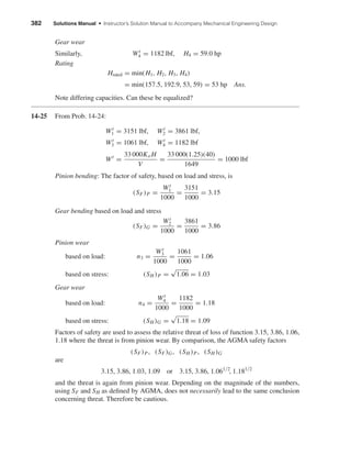
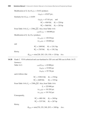
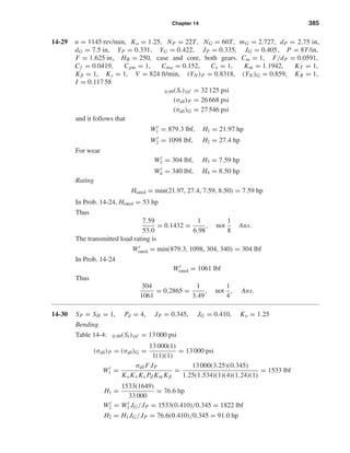
386. 386 Solutions Manual • Instructor’s Solution Manual to Accompany Mechanical Engineering Design
Wear
Table 14-8: Cp = 1960 psi
Table 14-7: 0.99(Sc)107 = 75 000 psi = (σc,all)P = (σc,all)G
Wt
3 =
(σc,all)P
Cp
2
FdpI
KoKv Ks KmCf
Wt
3 =
75 000
1960
2
3.25(5.5)(0.1176)
1.25(1.534)(1)(1.24)(1)
= 1295 lbf
Wt
4 = Wt
3 = 1295 lbf
H4 = H3 =
1295(1649)
33 000
= 64.7 hp
Rating
Hrated = min(76.7, 94.4, 64.7, 64.7) = 64.7 hp Ans.
Notice that the balance between bending and wear power is improved due to CI’s more
favorable Sc/St ratio. Also note that the life is 107
pinion revolutions which is (1/300) of
3(109
). Longer life goals require power derating.
14-31 From Table A-24a, Eav = 11.8(106
)
For φ = 14.5◦
and HB = 156
SC =
1.4(81)
2 sin 14.5°/[11.8(106)]
= 51 693 psi
For φ = 20◦
SC =
1.4(112)
2 sin 20°/[11.8(106)]
= 52 008 psi
SC = 0.32(156) = 49.9 kpsi
14-32 Programs will vary.
14-33
(YN )P = 0.977, (YN )G = 0.996
(St)P = (St)G = 82.3(250) + 12 150 = 32 725 psi
(σall)P =
32 725(0.977)
1(0.85)
= 37 615 psi
Wt
1 =
37 615(1.5)(0.423)
1(1.404)(1.043)(8.66)(1.208)(1)
= 1558 lbf
H1 =
1558(925)
33 000
= 43.7 hp
shi20396_ch14.qxd 8/20/03 12:43 PM Page 386

387. Chapter 14 387
(σall)G =
32 725(0.996)
1(0.85)
= 38 346 psi
Wt
2 =
38 346(1.5)(0.5346)
1(1.404)(1.043)(8.66)(1.208)(1)
= 2007 lbf
H2 =
2007(925)
33 000
= 56.3 hp
(ZN )P = 0.948, (ZN )G = 0.973
Table 14-6: 0.99(Sc)107 = 150 000 psi
(σc,allow)P = 150 000
0.948(1)
1(0.85)
= 167 294 psi
Wt
3 =
167 294
2300
2
1.963(1.5)(0.195)
1(1.404)(1.043)
= 2074 lbf
H3 =
2074(925)
33 000
= 58.1 hp
(σc,allow)G =
0.973
0.948
(167 294) = 171 706 psi
Wt
4 =
171 706
2300
2
1.963(1.5)(0.195)
1(1.404)(1.052)
= 2167 lbf
H4 =
2167(925)
33 000
= 60.7 hp
Hrated = min(43.7, 56.3, 58.1, 60.7) = 43.7 hp Ans.
Pinion bending controlling
14-34
(YN )P = 1.6831(108
)−0.0323
= 0.928
(YN )G = 1.6831(108
/3.059)−0.0323
= 0.962
Table 14-3: St = 55 000 psi
(σall)P =
55 000(0.928)
1(0.85)
= 60 047 psi
Wt
1 =
60 047(1.5)(0.423)
1(1.404)(1.043)(8.66)(1.208)(1)
= 2487 lbf
H1 =
2487(925)
33 000
= 69.7 hp
(σall)G =
0.962
0.928
(60 047) = 62 247 psi
Wt
2 =
62 247
60 047
0.5346
0.423
(2487) = 3258 lbf
H2 =
3258
2487
(69.7) = 91.3 hp
shi20396_ch14.qxd 8/20/03 12:43 PM Page 387

388. 388 Solutions Manual • Instructor’s Solution Manual to Accompany Mechanical Engineering Design
Table 14-6: Sc = 180 000 psi
(ZN )P = 2.466(108
)−0.056
= 0.8790
(ZN )G = 2.466(108
/3.059)−0.056
= 0.9358
(σc,all)P =
180 000(0.8790)
1(0.85)
= 186 141 psi
Wt
3 =
186 141
2300
2
1.963(1.5)(0.195)
1(1.404)(1.043)
= 2568 lbf
H3 =
2568(925)
33 000
= 72.0 hp
(σc,all)G =
0.9358
0.8790
(186 141) = 198 169 psi
Wt
4 =
198 169
186 141
2
1.043
1.052
(2568) = 2886 lbf
H4 =
2886(925)
33 000
= 80.9 hp
Hrated = min(69.7, 91.3, 72, 80.9) = 69.7 hp Ans.
Pinion bending controlling
14-35 (YN )P = 0.928, (YN )G = 0.962 (See Prob. 14-34)
Table 14-3: St = 65 000 psi
(σall)P =
65 000(0.928)
1(0.85)
= 70 965 psi
Wt
1 =
70 965(1.5)(0.423)
1(1.404)(1.043)(8.66)(1.208)
= 2939 lbf
H1 =
2939(925)
33 000
= 82.4 hp
(σall)G =
65 000(0.962)
1(0.85)
= 73 565 psi
Wt
2 =
73 565
70 965
0.5346
0.423
(2939) = 3850 lbf
H2 =
3850
2939
(82.4) = 108 hp
shi20396_ch14.qxd 8/20/03 12:43 PM Page 388

389. Chapter 14 389
Table 14-6: Sc = 225 000 psi
(ZN )P = 0.8790, (ZN )G = 0.9358
(σc,all)P =
225 000(0.879)
1(0.85)
= 232 676 psi
Wt
3 =
232 676
2300
2
1.963(1.5)(0.195)
1(1.404)(1.043)
= 4013 lbf
H3 =
4013(925)
33 000
= 112.5 hp
(σc,all)G =
0.9358
0.8790
(232 676) = 247 711 psi
Wt
4 =
247 711
232 676
2
1.043
1.052
(4013) = 4509 lbf
H4 =
4509(925)
33 000
= 126 hp
Hrated = min(82.4, 108, 112.5, 126) = 82.4 hp Ans.
The bending of the pinion is the controlling factor.
shi20396_ch14.qxd 8/20/03 12:43 PM Page 389

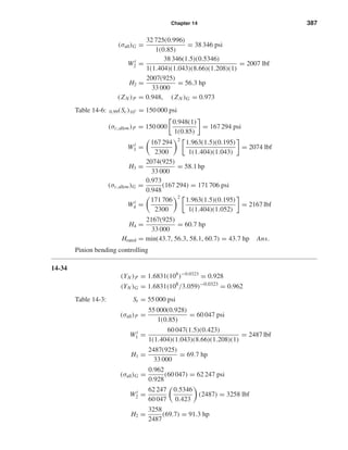
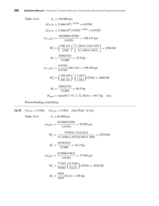
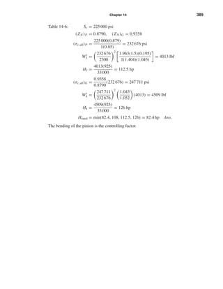
390. Chapter 15
15-1 Given: Uncrowned, through-hardened 300 Brinell core and case, Grade 1, NC = 109
rev of
pinion at R = 0.999, NP = 20 teeth, NG = 60 teeth, Qv = 6, Pd = 6 teeth/in, shaft angle
90°, np = 900 rev/min, JP = 0.249 and JG = 0.216 (Fig. 15-7), F = 1.25 in, SF =
SH = 1, Ko = 1.
Mesh dP = 20/6 = 3.333 in
dG = 60/6 = 10.000 in
Eq. (15-7): vt = π(3.333)(900/12) = 785.3 ft/min
Eq. (15-6): B = 0.25(12 − 6)2/3
= 0.8255
A = 50 + 56(1 − 0.8255) = 59.77
Eq. (15-5): Kv =
59.77 +
√
785.3
59.77
0.8255
= 1.374
Eq. (15-8): vt,max = [59.77 + (6 − 3)]2
= 3940 ft/min
Since 785.3 < 3904, Kv = 1.374 is valid. The size factor for bending is:
Eq. (15-10): Ks = 0.4867 + 0.2132/6 = 0.5222
For one gear straddle-mounted, the load-distribution factor is:
Eq. (15-11): Km = 1.10 + 0.0036(1.25)2
= 1.106
Eq. (15-15): (KL)P = 1.6831(109
)−0.0323
= 0.862
(KL)G = 1.6831(109
/3)−0.0323
= 0.893
Eq. (15-14): (CL)P = 3.4822(109
)−0.0602
= 1
(CL)G = 3.4822(109
/3)−0.0602
= 1.069
Eq. (15-19): KR = 0.50 − 0.25 log(1 − 0.999) = 1.25 (or Table 15-3)
CR = KR =
√
1.25 = 1.118
Bending
Fig. 15-13: 0.99St = sat = 44(300) + 2100 = 15 300 psi
Eq. (15-4): (σall)P = swt =
sat KL
SF KT KR
=
15 300(0.862)
1(1)(1.25)
= 10 551 psi
Eq. (15-3): Wt
P =
(σall)P FKx JP
Pd KoKv Ks Km
=
10 551(1.25)(1)(0.249)
6(1)(1.374)(0.5222)(1.106)
= 690 lbf
H1 =
690(785.3)
33 000
= 16.4 hp
Eq. (15-4): (σall)G =
15 300(0.893)
1(1)(1.25)
= 10 930 psi
shi20396_ch15.qxd 8/28/03 3:25 PM Page 390

391. Chapter 15 391
Wt
G =
10 930(1.25)(1)(0.216)
6(1)(1.374)(0.5222)(1.106)
= 620 lbf
H2 =
620(785.3)
33 000
= 14.8 hp Ans.
The gear controls the bending rating.
15-2 Refer to Prob. 15-1 for the gearset specifications.
Wear
Fig. 15-12: sac = 341(300) + 23 620 = 125 920 psi
For the pinion, CH = 1. From Prob. 15-1, CR = 1.118. Thus, from Eq. (15-2):
(σc,all)P =
sac(CL)PCH
SH KT CR
(σc,all)P =
125 920(1)(1)
1(1)(1.118)
= 112 630 psi
For the gear, from Eq. (15-16),
B1 = 0.008 98(300/300) − 0.008 29 = 0.000 69
CH = 1 + 0.000 69(3 − 1) = 1.001 38
And Prob. 15-1, (CL)G = 1.0685. Equation (15-2) thus gives
(σc,all)G =
sac(CL)GCH
SH KT CR
(σc,all)G =
125 920(1.0685)(1.001 38)
1(1)(1.118)
= 120 511 psi
For steel: Cp = 2290 psi
Eq. (15-9): Cs = 0.125(1.25) + 0.4375 = 0.593 75
Fig. 15-6: I = 0.083
Eq. (15-12): Cxc = 2
Eq. (15-1): Wt
P =
(σc,all)P
Cp
2
FdP I
KoKv KmCsCxc
=
112 630
2290
2
1.25(3.333)(0.083)
1(1.374)(1.106)(0.5937)(2)
= 464 lbf
H3 =
464(785.3)
33 000
= 11.0 hp
Wt
G =
120 511
2290
2
1.25(3.333)(0.083)
1(1.374)(1.106)(0.593 75)(2)
= 531 lbf
H4 =
531(785.3)
33 000
= 12.6 hp
shi20396_ch15.qxd 8/28/03 3:25 PM Page 391

392. 392 Solutions Manual • Instructor’s Solution Manual to Accompany Mechanical Engineering Design
The pinion controls wear: H = 11.0 hp Ans.
The power rating of the mesh, considering the power ratings found in Prob. 15-1, is
H = min(16.4, 14.8, 11.0, 12.6) = 11.0 hp Ans.
15-3 AGMA 2003-B97 does not fully address cast iron gears, however, approximate compar-
isons can be useful. This problem is similar to Prob. 15-1, but not identical. We will orga-
nize the method. A follow-up could consist of completing Probs. 15-1 and 15-2 with
identical pinions, and cast iron gears.
Given: Uncrowned, straight teeth, Pd = 6 teeth/in, NP = 30 teeth, NG = 60 teeth, ASTM
30 cast iron, material Grade 1, shaft angle 90°, F = 1.25, nP = 900 rev/min, φn = 20◦,
one gear straddle-mounted, Ko = 1, JP = 0.268, JG = 0.228, SF = 2, SH =
√
2.
Mesh dP = 30/6 = 5.000 in
dG = 60/6 = 10.000 in
vt = π(5)(900/12) = 1178 ft/min
Set NL = 107
cycles for the pinion. For R = 0.99,
Table 15-7: sat = 4500 psi
Table 15-5: sac = 50 000 psi
Eq. (15-4): swt =
sat KL
SF KT KR
=
4500(1)
2(1)(1)
= 2250 psi
The velocity factor Kv represents stress augmentation due to mislocation of tooth profiles
along the pitch surface and the resulting “falling” of teeth into engagement. Equation (5-67)
shows that the induced bending moment in a cantilever (tooth) varies directly with
√
E of the
tooth material. If only the material varies (cast iron vs. steel) in the same geometry, I is the
same. From the Lewis equation of Section 14-1,
σ =
M
I/c
=
KvWt P
FY
We expect the ratio σCI/σsteel to be
σCI
σsteel
=
(Kv)CI
(Kv)steel
=
ECI
Esteel
In the case of ASTM class 30, from Table A-24(a)
(ECI)av = (13 + 16.2)/2 = 14.7 kpsi
Then
(Kv)CI =
14.7
30
(Kv)steel = 0.7(Kv)steel
shi20396_ch15.qxd 8/28/03 3:25 PM Page 392

393. Chapter 15 393
Our modeling is rough, but it convinces us that (Kv)CI < (Kv)steel, but we are not sure of
the value of (Kv)CI. We will use Kv for steel as a basis for a conservative rating.
Eq. (15-6): B = 0.25(12 − 6)2/3
= 0.8255
A = 50 + 56(1 − 0.8255) = 59.77
Eq. (15-5): Kv =
59.77 +
√
1178
59.77
0.8255
= 1.454
Pinion bending (σall)P = swt = 2250 psi
From Prob. 15-1, Kx = 1, Km = 1.106, Ks = 0.5222
Eq. (15-3): Wt
P =
(σall)P FKx JP
Pd KoKv Ks Km
=
2250(1.25)(1)(0.268)
6(1)(1.454)(0.5222)(1.106)
= 149.6 lbf
H1 =
149.6(1178)
33 000
= 5.34 hp
Gear bending
Wt
G = Wt
P
JG
JP
= 149.6
0.228
0.268
= 127.3 lbf
H2 =
127.3(1178)
33 000
= 4.54 hp
The gear controls in bending fatigue.
H = 4.54 hp Ans.
15-4 Continuing Prob. 15-3,
Table 15-5: sac = 50 000 psi
swt = σc,all =
50 000
√
2
= 35 355 psi
Eq. (15-1): Wt
=
σc,all
Cp
2
FdP I
KoKv KmCsCxc
Fig. 15-6: I = 0.86
From Probs. 15-1 and 15-2: Cs = 0.593 75, Ks = 0.5222, Km = 1.106, Cxc = 2
From Table 14-8: Cp = 1960 psi
Thus, Wt
=
35 355
1960
2
1.25(5.000)(0.086)
1(1.454)(1.106)(0.59375)(2)
= 91.6 lbf
H3 = H4 =
91.6(1178)
33 000
= 3.27 hp
shi20396_ch15.qxd 8/28/03 3:25 PM Page 393

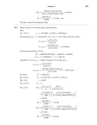
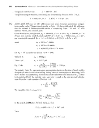
394. 394 Solutions Manual • Instructor’s Solution Manual to Accompany Mechanical Engineering Design
Rating Based on results of Probs. 15-3 and 15-4,
H = min(5.34, 4.54, 3.27, 3.27) = 3.27 hp Ans.
The mesh is weakest in wear fatigue.
15-5 Uncrowned, through-hardened to 180 Brinell (core and case), Grade 1, 109
rev of pinion at
R = 0.999, Np = z1 = 22 teeth, Na = z2 = 24 teeth, Qv = 5, met = 4 mm, shaft angle
90°, n1 = 1800 rev/min, SF = 1, SH = SF =
√
1, JP = YJ1 = 0.23, JG = YJ2 =
0.205, F = b = 25 mm, Ko = KA = KT = Kθ = 1 and Cp = 190
√
MPa.
Mesh dP = de1 = mz1 = 4(22) = 88 mm
dG = met z2 = 4(24) = 96 mm
Eq. (15-7): vet = 5.236(10−5
)(88)(1800) = 8.29 m/s
Eq. (15-6): B = 0.25(12 − 5)2/3
= 0.9148
A = 50 + 56(1 − 0.9148) = 54.77
Eq. (15-5): Kv =
54.77 +
√
200(8.29)
54.77
0.9148
= 1.663
Eq. (15-10): Ks = Yx = 0.4867 + 0.008 339(4) = 0.520
Eq. (15-11) with Kmb = 1 (both straddle-mounted),
Km = KHβ = 1 + 5.6(10−6
)(252
) = 1.0035
From Fig. 15-8,
(CL)P = (ZNT )P = 3.4822(109
)−0.0602
= 1.00
(CL)G = (ZNT )G = 3.4822[109
(22/24)]−0.0602
= 1.0054
Eq. (15-12): Cxc = Zxc = 2 (uncrowned)
Eq. (15-19): KR = YZ = 0.50 − 0.25 log (1 − 0.999) = 1.25
CR = ZZ = YZ =
√
1.25 = 1.118
From Fig. 15-10, CH = Zw = 1
Eq. (15-9): Zx = 0.004 92(25) + 0.4375 = 0.560
Wear of Pinion
Fig. 15-12: σH lim = 2.35HB + 162.89
= 2.35(180) + 162.89 = 585.9 MPa
Fig. 15-6: I = ZI = 0.066
Eq. (15-2): (σH )P =
(σH lim)P(ZNT )P ZW
SH Kθ ZZ
=
585.9(1)(1)
√
1(1)(1.118)
= 524.1 MPa
Wt
P =
σH
Cp
2
bde1 ZI
1000KA Kv KHβ Zx Zxc
shi20396_ch15.qxd 8/28/03 3:25 PM Page 394

395. Chapter 15 395
The constant 1000 expresses Wt in kN
Wt
P =
524.1
190
2
25(88)(0.066)
1000(1)(1.663)(1.0035)(0.56)(2)
= 0.591 kN
H3 =
Wtrn1
9.55
=
0.591(88/2)(1800)
9.55(10)3
= 4.90 kW
Wear of Gear σH lim = 585.9 MPa
(σH )G =
585.9(1.0054)
√
1(1)(1.118)
= 526.9 MPa
Wt
G = Wt
P
(σH )G
(σH )P
= 0.591
526.9
524.1
= 0.594 kN
H4 =
Wtrn
9.55
=
0.594(88/2)(1800)
9.55(103)
= 4.93 kW
Thus in wear, the pinion controls the power rating; H = 4.90 kW Ans.
We will rate the gear set after solving Prob. 15-6.
15-6 Refer to Prob. 15-5 for terms not defined below.
Bending of Pinion
(KL)P = (YNT )P = 1.6831(109
)−0.0323
= 0.862
(KL)G = (YNT )G = 1.6831[109
(22/24)]−0.0323
= 0.864
Fig. 15-13: σF lim = 0.30HB + 14.48
= 0.30(180) + 14.48 = 68.5 MPa
Eq. (15-13): Kx = Yβ = 1
From Prob. 15-5: YZ = 1.25, vet = 8.29 m/s
Kv = 1.663, Kθ = 1, Yx = 0.56, KHβ = 1.0035
(σF)P =
σF limYNT
SF Kθ YZ
=
68.5(0.862)
1(1)(1.25)
= 47.2 MPa
Wt
p =
(σF)PbmetYβYJ1
1000KA KvYx KHβ
=
47.2(25)(4)(1)(0.23)
1000(1)(1.663)(0.56)(1.0035)
= 1.16 kN
H1 =
1.16(88/2)(1800)
9.55(103)
= 9.62 kW
Bending of Gear
σF lim = 68.5 MPa
(σF)G =
68.5(0.864)
1(1)(1.25)
= 47.3 MPa
Wt
G =
47.3(25)(4)(1)(0.205)
1000(1)(1.663)(0.56)(1.0035)
= 1.04 kN
H2 =
1.04(88/2)(1800)
9.55(103)
= 8.62 kW
shi20396_ch15.qxd 8/28/03 3:25 PM Page 395

396. 396 Solutions Manual • Instructor’s Solution Manual to Accompany Mechanical Engineering Design
Rating of mesh is
Hrating = min(9.62, 8.62, 4.90, 4.93) = 4.90 kW Ans.
with pinion wear controlling.
15-7
(a) (SF)P =
σall
σ P
= (SF)G =
σall
σ G
(sat KL/KT KR)P
(Wt Pd KoKv Ks Km/FKx J)P
=
(sat KL/KT KR)G
(Wt Pd KoKv Ks Km/FKx J)G
All terms cancel except for sat, KL , and J,
(sat)P(KL)P JP = (sat)G(KL)G JG
From which
(sat)G =
(sat)P(KL)P JP
(KL)G JG
= (sat)P
JP
JG
m
β
G
Where β = −0.0178 or β = −0.0323 as appropriate. This equation is the same as
Eq. (14-44). Ans.
(b) In bending
Wt
=
σall
SF
FKx J
Pd KoKv Ks Km 11
=
sat
SF
KL
KT KR
FKx J
Pd KoKv Ks Km 11
(1)
In wear
sacCLCU
SH KT CR 22
= Cp
Wt KoKv KmCsCxc
FdP I
1/2
22
Squaring and solving for Wt
gives
Wt
=
s2
acC2
LC2
H
S2
H K2
T C2
RC2
P 22
FdP I
KoKv KmCsCxc 22
(2)
Equating the right-hand sides of Eqs. (1) and (2) and canceling terms, and recognizing
that CR = KR and PddP = NP,
we obtain
(sac)22 =
Cp
(CL)22
S2
H
SF
(sat)11(KL)11Kx J11KT CsCxc
C2
H NP Ks I
For equal Wt
in bending and wear
S2
H
SF
=
√
SF
2
SF
= 1
So we get
(sac)G =
Cp
(CL)GCH
(sat)P(KL)P JP Kx KT CsCxc
NP I Ks
Ans.
shi20396_ch15.qxd 8/28/03 3:25 PM Page 396

397. Chapter 15 397
(c)
(SH )P = (SH )G =
σc,all
σc P
=
σc,all
σc G
Substituting in the right-hand equality gives
[sacCL/(CR KT )]P
Cp Wt KoKv KmCsCxc/(FdP I)
P
=
[sacCLCH /(CR KT )]G
Cp Wt KoKv KmCsCxc/(FdP I)
G
Denominators cancel leaving
(sac)P(CL)P = (sac)G(CL)GCH
Solving for (sac)P gives, with CH
.
= 1
(sac)P = (sac)G
(CL)G
(CL)P
CH
.
= (sac)G
1
mG
−0.0602
(1)
(sac)P
.
= (sac)Gm0.0602
G Ans.
This equation is the transpose of Eq. (14-45).
15-8
Core Case
Pinion (HB)11 (HB)12
Gear (HB)21 (HB)22
Given (HB)11 = 300 Brinell
Eq. (15-23): (sat)P = 44(300) + 2100 = 15 300 psi
(sat)G(sat)P
JP
JG
m−0.0323
G = 15 300
0.249
0.216
3−0.0323
= 17 023 psi
(HB)21 =
17 023 − 2100
44
= 339 Brinell Ans.
(sac)G =
2290
1.0685(1)
15 300(0.862)(0.249)(1)(0.593 25)(2)
20(0.086)(0.5222)
= 141 160 psi
(HB)22 =
141 160 − 23 600
341
= 345 Brinell Ans.
(sac)P = (sac)Gm0.0602
G
1
CH
.
= 141 160(30.0602
)
1
1
= 150 811 psi
(HB)12 =
150 811 − 23 600
341
= 373 Brinell Ans.
Care Case
Pinion 300 373 Ans.
Gear 399 345
shi20396_ch15.qxd 8/28/03 3:25 PM Page 397

398. 398 Solutions Manual • Instructor’s Solution Manual to Accompany Mechanical Engineering Design
15-9 Pinion core
(sat)P = 44(300) + 2100 = 15 300 psi
(σall)P =
15 300(0.862)
1(1)(1.25)
= 10 551 psi
Wt
=
10 551(1.25)(0.249)
6(1)(1.374)(0.5222)(1.106)
= 689.7 lbf
Gear core
(sat)G = 44(352) + 2100 = 17 588 psi
(σall)G =
17 588(0.893)
1(1)(1.25)
= 12 565 psi
Wt
=
12 565(1.25)(0.216)
6(1)(1.374)(0.5222)(1.106)
= 712.5 lbf
Pinion case
(sac)P = 341(372) + 23 620 = 150 472 psi
(σc,all)P =
150 472(1)
1(1)(1.118)
= 134 590 psi
Wt
=
134 590
2290
2
1.25(3.333)(0.086)
1(1.374)(1.106)(0.593 75)(2)
= 685.8 lbf
Gear case
(sac)G = 341(344) + 23 620 = 140 924 psi
(σc,all)G =
140 924(1.0685)(1)
1(1)(1.118)
= 134 685 psi
W t
=
134 685
2290
2
1.25(3.333)(0.086)
1(1.374)(1.106)(0.593 75)(2)
= 686.8 lbf
The rating load would be
Wt
rated = min(689.7, 712.5, 685.8, 686.8) = 685.8 lbf
which is slightly less than intended.
Pinion core
(sat)P = 15 300 psi (as before)
(σall)P = 10 551 (as before)
Wt
= 689.7 (as before)
Gear core
(sat)G = 44(339) + 2100 = 17 016 psi
(σall)G =
17 016(0.893)
1(1)(1.25)
= 12 156 psi
Wt
=
12 156(1.25)(0.216)
6(1)(1.374)(0.5222)(1.106)
= 689.3 lbf
shi20396_ch15.qxd 8/28/03 3:25 PM Page 398

399. Chapter 15 399
Pinion case
(sac)P = 341(373) + 23 620 = 150 813 psi
(σc,all)P =
150 813(1)
1(1)(1.118)
= 134 895 psi
Wt
=
134 895
2290
2
1.25(3.333)(0.086)
1(1.374)(1.106)(0.593 75)(2)
= 689.0 lbf
Gear case
(sac)G = 341(345) + 23 620 = 141 265 psi
(σc,all)G =
141 265(1.0685)(1)
1(1)(1.118)
= 135 010 psi
Wt
=
135 010
2290
2
1.25(3.333)(0.086)
1(1.1374)(1.106)(0.593 75)(2)
= 690.1 lbf
The equations developed within Prob. 15-7 are effective. In bevel gears, the gear tooth
is weaker than the pinion so (CH )G = 1. (See p. 784.) Thus the approximations in
Prob. 15-7 with CH = 1 are really still exact.
15-10 The catalog rating is 5.2 hp at 1200 rev/min for a straight bevel gearset. Also given:
NP = 20 teeth, NG = 40 teeth, φn = 20◦
, F = 0.71 in, JP = 0.241, JG = 0.201,
Pd = 10 teeth/in, through-hardened to 300 Brinell-General Industrial Service, and
Qv = 5 uncrowned.
Mesh
dP = 20/10 = 2.000 in, dG = 40/10 = 4.000 in
vt =
πdPnP
12
=
π(2)(1200)
12
= 628.3 ft/min
Ko = 1, SF = 1, SH = 1
Eq. (15-6): B = 0.25(12 − 5)2/3
= 0.9148
A = 50 + 56(1 − 0.9148) = 54.77
Eq. (15-5): Kv =
54.77 +
√
628.3
54.77
0.9148
= 1.412
Eq. (15-10): Ks = 0.4867 + 0.2132/10 = 0.508
Kmb = 1.25
Eq. (15-11): Km = 1.25 + 0.0036(0.71)2
= 1.252
Eq. (15-15): (KL)P = 1.6831(109
)−0.0323
= 0.862
(KL)G = 1.6831(109
/2)−0.0323
= 0.881
Eq. (15-14): (CL)P = 3.4822(109
)−0.0602
= 1.000
(CL)G = 3.4822(109
/2)−0.0602
= 1.043
shi20396_ch15.qxd 8/28/03 3:25 PM Page 399

400. 400 Solutions Manual • Instructor’s Solution Manual to Accompany Mechanical Engineering Design
Analyze for 109
pinion cycles at 0.999 reliability
Eq. (15-19): KR = 0.50 − 0.25 log(1 − 0.999) = 1.25
CR = KR =
√
1.25 = 1.118
Bending
Pinion:
Eq. (15-23): (sat)P = 44(300) + 2100 = 15 300 psi
Eq. (15-4): (σall)P =
15 300(0.862)
1(1)(1.25)
= 10 551 psi
Eq. (15-3): Wt
=
(σall)P FKx JP
Pd KoKv Ks Km
=
10 551(0.71)(1)(0.241)
10(1)(1.412)(0.508)(1.252)
= 201 lbf
H1 =
201(628.3)
33 000
= 3.8 hp
Gear:
(sat)G = 15 300 psi
Eq. (15-4): (σall)G =
15 300(0.881)
1(1)(1.25)
= 10 783 psi
Eq. (15-3): Wt
=
10 783(0.71)(1)(0.201)
10(1)(1.412)(0.508)(1.252)
= 171.4 lbf
H2 =
171.4(628.3)
33 000
= 3.3 hp
Wear
Pinion:
(CH )G = 1, I = 0.078, Cp = 2290 psi, Cxc = 2
Cs = 0.125(0.71) + 0.4375 = 0.526 25
Eq. (15-22): (sac)P = 341(300) + 23 620 = 125 920 psi
(σc,all)P =
125 920(1)(1)
1(1)(1.118)
= 112 630 psi
Eq. (15-1): Wt
=
(σc,all)P
Cp
2
FdP I
KoKv KmCsCxc
=
112 630
2290
2
0.71(2.000)(0.078)
1(1.412)(1.252)(0.526 25)(2)
= 144.0 lbf
H3 =
144(628.3)
33 000
= 2.7 hp
shi20396_ch15.qxd 8/28/03 3:25 PM Page 400

401. Chapter 15 401
Gear:
(sac)G = 125 920 psi
(σc,all) =
125 920(1.043)(1)
1(1)(1.118)
= 117 473 psi
Wt
=
117 473
2290
2
0.71(2.000)(0.078)
1(1.412)(1.252)(0.526 25)(2)
= 156.6 lbf
H4 =
156.6(628.3)
33 000
= 3.0 hp
Rating:
H = min(3.8, 3.3, 2.7, 3.0) = 2.7 hp
Pinion wear controls the power rating. While the basis of the catalog rating is unknown,
it is overly optimistic (by a factor of 1.9).
15-11 From Ex. 15-1, the core hardness of both the pinion and gear is 180 Brinell. So (HB)11
and (HB)21 are 180 Brinell and the bending stress numbers are:
(sat)P = 44(180) + 2100 = 10 020 psi
(sat)G = 10 020 psi
The contact strength of the gear case, based upon the equation derived in Prob. 15-7, is
(sac)G =
Cp
(CL)GCH
S2
H
SF
(sat)P(KL)P Kx JP KT CsCxc
NP I Ks
Substituting (sat)P from above and the values of the remaining terms from Ex. 15-1,
2290
1.32(1)
1.52
1.5
10 020(1)(1)(0.216)(1)(0.575)(2)
25(0.065)(0.529)
= 114 331 psi
(HB)22 =
114 331 − 23 620
341
= 266 Brinell
The pinion contact strength is found using the relation from Prob. 15-7:
(sac)P = (sac)Gm0.0602
G CH = 114 331(1)0.0602
(1) = 114 331 psi
(HB)12 =
114 331 − 23 600
341
= 266 Brinell
Core Case
Pinion 180 266
Gear 180 266
Realization of hardnesses
The response of students to this part of the question would be a function of the extent
to which heat-treatment procedures were covered in their materials and manufacturing
shi20396_ch15.qxd 8/28/03 3:25 PM Page 401

402. prerequisites, and how quantitative it was. The most important thing is to have the stu-
dent think about it.
The instructor can comment in class when students curiosity is heightened. Options
that will surface may include:
• Select a through-hardening steel which will meet or exceed core hardness in the hot-
rolled condition, then heat-treating to gain the additional 86 points of Brinell hardness
by bath-quenching, then tempering, then generating the teeth in the blank.
• Flame or induction hardening are possibilities.
• The hardness goal for the case is sufficiently modest that carburizing and case harden-
ing may be too costly. In this case the material selection will be different.
• The initial step in a nitriding process brings the core hardness to 33–38 Rockwell
C-scale (about 300–350 Brinell) which is too much.
Emphasize that development procedures are necessary in order to tune the “BlackArt”
to the occasion. Manufacturing personnel know what to do and the direction of adjust-
ments, but how much is obtained by asking the gear (or gear blank). Refer your students
to D. W. Dudley, Gear Handbook, library reference section, for descriptions of heat-treat-
ing processes.
15-12 Computer programs will vary.
15-13 A design program would ask the user to make the a priori decisions, as indicated in
Sec. 15-5, p. 794, MED7. The decision set can be organized as follows:
A priori decisions
• Function: H, Ko, rpm, mG, temp., NL, R
• Design factor: nd (SF = nd, SH =
√
nd)
• Tooth system: Involute, Straight Teeth, Crowning, φn
• Straddling: Kmb
• Tooth count: NP(NG = mG NP)
Design decisions
• Pitch and Face: Pd, F
• Quality number: Qv
• Pinion hardness: (HB)1, (HB)3
• Gear hardness: (HB)2, (HB)4
402 Solutions Manual • Instructor’s Solution Manual to Accompany Mechanical Engineering Design
shi20396_ch15.qxd 8/28/03 3:25 PM Page 402

403. 403
Firstgatheralloftheequationsoneneeds,thenarrangethembeforecoding.Findtherequiredhardnesses,expresstheconsequencesofthe
chosenhardnesses,andallowforrevisionsasappropriate.
PinionBendingGearBendingPinionWearGearWear
Load-inducedσ=
Wt
PKoKvKmKs
FKxJP
=s11σ=
Wt
PKoKvKmKs
FKxJG
=s21σc=Cp
Wt
KoKvCsCxc
FdPI
1/2
=s12s22=s12
stress(Allowable
stress)
Tabulated(sat)P=
s11SFKTKR
(KL)P
(sat)G=
s21SFKTKR
(KL)G
(sac)P=
s12SHKTCR
(CL)P(CH)P
(sac)G=
s22SHKTCR
(CL)G(CH)Gstrength
Associatedbhn=



(sat)P−2100
44
(sat)P−5980
48
bhn=



(sat)G−2100
44
(sat)G−5980
48
bhn=



(sac)P−23620
341
(sac)P−29560
363.6
bhn=



(sac)G−23620
341
(sac)G−29560
363.6
hardness
Chosen(HB)11(HB)21(HB)12(HB)22
hardness
Newtabulated(sat1)P=44(HB)11+2100
48(HB)11+5980
(sat1)G=44(HB)21+2100
48(HB)21+5980
(sac1)P=341(HB)12+23620
363.6(HB)12+29560
(sac1)G=341(HB)22+23620
363.6(HB)22+29560strength
Factorofn11=
σall
σ
=
(sat1)P(KL)P
s11KTKR
n21=
(sat1)G(KL)G
s21KTKR
n12=
(sac1)P(CL)P(CH)P
s12KTCR
2
n22=
(sac1)G(CL)G(CH)G
s22KTCR
2
safety
Note:SF=nd,SH=SF
shi20396_ch15.qxd 8/28/03 3:25 PM Page 403

404. 404 Solutions Manual • Instructor’s Solution Manual to Accompany Mechanical Engineering Design
15-14 NW = 1, NG = 56, Pt = 8 teeth/in, dP = 1.5 in, Ho = 1hp, φn = 20◦
, ta = 70◦
F,
Ka = 1.25, nd = 1, Fe = 2 in, A = 850 in2
(a) mG = NG/NW = 56, dG = NG/Pt = 56/8 = 7.0 in
px = π/8 = 0.3927 in, C = 1.5 + 7 = 8.5 in
Eq. (15-39): a = px/π = 0.3927/π = 0.125 in
Eq. (15-40): h = 0.3683px = 0.1446 in
Eq. (15-41): ht = 0.6866px = 0.2696 in
Eq. (15-42): do = 1.5 + 2(0.125) = 1.75 in
Eq. (15-43): dr = 3 − 2(0.1446) = 2.711 in
Eq. (15-44): Dt = 7 + 2(0.125) = 7.25 in
Eq. (15-45): Dr = 7 − 2(0.1446) = 6.711 in
Eq. (15-46): c = 0.1446 − 0.125 = 0.0196 in
Eq. (15-47): (FW )max = 2
7.25
2
2
−
7
2
− 0.125
2
= 2.646 in
VW = π(1.5)(1725/12) = 677.4 ft/min
VG =
π(7)(1725/56)
12
= 56.45 ft/min
Eq. (13-28): L = px NW = 0.3927 in, λ = tan−1 0.3927
π(1.5)
= 4.764◦
Pn =
Pt
cos λ
=
8
cos 4.764°
= 8.028
pn =
π
Pn
= 0.3913 in
Eq. (15-62): Vs =
π(1.5)(1725)
12 cos 4.764°
= 679.8 ft/min
(b) Eq. (15-38): f = 0.103 exp −0.110(679.8)0.450
+ 0.012 = 0.0250
Eq. (13-46):
e =
cos φn − f tan λ
cos φn + f cot λ
=
cos 20° − 0.0250 tan 4.764°
cos 20° + 0.0250 cot 4.764°
= 0.7563 Ans.
Eq. (15-58): Wt
G =
33 000 nd HoKa
VGe
=
33 000(1)(1)(1.25)
56.45(0.7563)
= 966 lbf Ans.
Eq. (15-57): Wt
W = Wt
G
cos φn sin λ + f cos λ
cos φn cos λ − f sin λ
= 966
cos 20° sin 4.764° + 0.025 cos 4.764°
cos 20° cos 4.764° − 0.025 sin 4.764°
= 106.4 lbf Ans.
shi20396_ch15.qxd 8/28/03 3:25 PM Page 404

405. Chapter 15 405
(c) Eq. (15-33): Cs = 1190 − 477 log 7.0 = 787
Eq. (15-36): Cm = 0.0107 −562 + 56(56) + 5145 = 0.767
Eq. (15-37): Cv = 0.659 exp[−0.0011(679.8)] = 0.312
Eq. (15-38): (Wt
)all = 787(7)0.8
(2)(0.767)(0.312) = 1787 lbf
Since Wt
G < (Wt
)all, the mesh will survive at least 25000 h.
Eq. (15-61): Wf =
0.025(966)
0.025 sin 4.764° − cos 20° cos 4.764°
= −29.5 lbf
Eq. (15-63): Hf =
29.5(679.8)
33 000
= 0.608 hp
HW =
106.4(677.4)
33 000
= 2.18 hp
HG =
966(56.45)
33 000
= 1.65 hp
The mesh is sufficient Ans.
Pn = Pt/cos λ = 8/cos 4.764◦
= 8.028
pn = π/8.028 = 0.3913 in
σG =
966
0.3913(0.5)(0.125)
= 39 500 psi
The stress is high. At the rated horsepower,
σG =
1
1.65
39 500 = 23 940 psi acceptable
(d) Eq. (15-52): Amin = 43.2(8.5)1.7
= 1642 in2
< 1700 in2
Eq. (15-49): Hloss = 33 000(1 − 0.7563)(2.18) = 17 530 ft · lbf/min
Assuming a fan exists on the worm shaft,
Eq. (15-50): ¯hC R =
1725
3939
+ 0.13 = 0.568 ft · lbf/(min · in2
· ◦
F)
Eq. (15-51): ts = 70 +
17 530
0.568(1700)
= 88.2◦
F Ans.
shi20396_ch15.qxd 8/28/03 3:25 PM Page 405

406. 406
15-15to15-22
Problemstatementvaluesof25hp,1125rev/min,mG=10,Ka=1.25,nd=1.1,φn=20°,ta=70°Farenotreferencedinthetable.
Parameters
Selected15-1515-1615-1715-1815-1915-2015-2115-22
#1px1.751.751.751.751.751.751.751.75
#2dW3.603.603.603.603.604.103.603.60
#3FG2.401.681.431.692.402.252.42.4
#4A20002000200020002000200025002600
FANFAN
HW38.238.238.238.238.238.041.241.2
HG36.236.236.236.236.236.137.737.7
Hf1.871.471.971.971.971.853.593.59
NW33333333
NG3030303030303030
KW1258050115185
Cs6078541000
Cm0.7590.7590.759
Cv0.2360.2360.236
VG492492492492492563492492
Wt
G24302430243024302430212025242524
Wt
W11891189118911891189103812841284
f0.01930.01930.01930.01930.01930.01830.034A0.034A
e0.9480.9480.9480.9480.9480.9510.913A0.913A
(Pt)G1.7951.7951.7951.7951.7951.5711.7951.795
Pn1.9791.9791.9791.9791.9791.7321.9791.979
C-to-C10.15610.15610.15610.15610.15611.610.15610.156
ts177177177177177171179.6179.6
L5.255.255.255.255.256.05.255.25
λ24.924.924.924.924.924.9824.924.9
σG51037290856572475103415853015301
dG16.7116.7116.7116.7116.7119.09916.716.71
shi20396_ch15.qxd 8/28/03 3:25 PM Page 406

407. Chapter 16
16-1
(a) θ1 = 0°, θ2 = 120°, θa = 90°, sin θa = 1, a = 5 in
Eq. (16-2): Mf =
0.28pa(1.5)(6)
1
120°
0°
sin θ(6 − 5 cos θ) dθ
= 17.96pa lbf · in
Eq. (16-3): MN =
pa(1.5)(6)(5)
1
120°
0°
sin2
θ dθ = 56.87pa lbf · in
c = 2(5 cos 30◦
) = 8.66 in
Eq. (16-4): F =
56.87pa − 17.96pa
8.66
= 4.49pa
pa = F/4.49 = 500/4.49 = 111.4 psi for cw rotation
Eq. (16-7): 500 =
56.87pa + 17.96pa
8.66
pa = 57.9 psi for ccw rotation
A maximum pressure of 111.4 psioccurs on the RH shoe for cw rotation. Ans.
(b) RH shoe:
Eq. (16-6): TR =
0.28(111.4)(1.5)(6)2
(cos 0◦ − cos 120◦)
1
= 2530 lbf · in Ans.
LH shoe:
Eq. (16-6): TL =
0.28(57.9)(1.5)(6)2
(cos 0◦ − cos 120◦)
1
= 1310 lbf · in Ans.
Ttotal = 2530 + 1310 = 3840 lbf · in Ans.
(c) Force vectors not to scale
x
y
Fy
Ry
Rx
R
Fx
F
Secondary
shoe
30Њ
y
x
Rx
Fy
Fx
F
Ry
R
Primary
shoe
30Њ
shi20396_ch16.qxd 8/28/03 4:01 PM Page 407

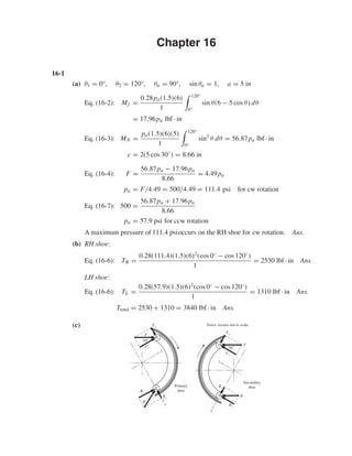
408. 408 Solutions Manual • Instructor’s Solution Manual to Accompany Mechanical Engineering Design
RH shoe: Fx = 500 sin 30° = 250 lbf, Fy = 500 cos 30° = 433 lbf
Eqs. (16-8): A =
1
2
sin2
θ
120◦
0◦
= 0.375, B =
θ
2
−
1
4
sin 2θ
2π/3 rad
0
= 1.264
Eqs. (16-9): Rx =
111.4(1.5)(6)
1
[0.375 − 0.28(1.264)] − 250 = −229 lbf
Ry =
111.4(1.5)(6)
1
[1.264 + 0.28(0.375)] − 433 = 940 lbf
R = [(−229)2
+ (940)2
]1/2
= 967 lbf Ans.
LH shoe: Fx = 250 lbf, Fy = 433 lbf
Eqs. (16-10): Rx =
57.9(1.5)(6)
1
[0.375 + 0.28(1.264)] − 250 = 130 lbf
Ry =
57.9(1.5)(6)
1
[1.264 − 0.28(0.375)] − 433 = 171 lbf
R = [(130)2
+ (171)2
]1/2
= 215 lbf Ans.
16-2 θ1 = 15°, θ2 = 105°, θa = 90°, sin θa = 1, a = 5 in
Eq. (16-2): Mf =
0.28pa(1.5)(6)
1
105°
15°
sin θ(6 − 5 cos θ) dθ = 13.06pa
Eq. (16-3): MN =
pa(1.5)(6)(5)
1
105°
15°
sin2
θ dθ = 46.59pa
c = 2(5 cos 30°) = 8.66 in
Eq. (16-4): F =
46.59pa − 13.06pa
8.66
= 3.872pa
RH shoe:
pa = 500/3.872 = 129.1 psi on RH shoe for cw rotation Ans.
Eq. (16-6): TR =
0.28(129.1)(1.5)(62
)(cos 15° − cos 105°)
1
= 2391 lbf · in
LH shoe:
500 =
46.59pa + 13.06pa
8.66
⇒ pa = 72.59 psi on LH shoe for ccw rotation Ans.
TL =
0.28(72.59)(1.5)(62
)(cos 15° − cos 105°)
1
= 1344 lbf · in
Ttotal = 2391 + 1344 = 3735 lbf · in Ans.
Comparing this result with that of Prob. 16-1, a 2.7% reduction in torque is achieved by
using 25% less braking material.
shi20396_ch16.qxd 8/28/03 4:01 PM Page 408

409. Chapter 16 409
16-3 Given: θ1 = 0°, θ2 = 120°, θa = 90°, sin θa = 1, a = R = 90 mm, f = 0.30,
F = 1000 N = 1 kN, r = 280/2 = 140 mm, counter-clockwise rotation.
LH shoe:
Mf =
f pabr
sin θa
r(1 − cos θ2) −
a
2
sin2
θ2
=
0.30pa(0.030)(0.140)
1
0.140(1 − cos 120◦
) −
0.090
2
sin2
120°
= 0.000 222pa N · m
MN =
pabra
sin θa
θ2
2
−
1
4
sin 2θ2
=
pa(0.030)(0.140)(0.090)
1
120°
2
π
180
−
1
4
sin 2(120°)
= 4.777(10−4
) pa N · m
c = 2r cos
180◦ − θ2
2
= 2(0.090) cos 30◦
= 0.155 88 m
F = 1 = pa
4.777(10−4
) − 2.22(10−4
)
0.155 88
= 1.64(10−3
) pa
pa = 1/1.64(10−3
) = 610 kPa
TL =
f pabr2
(cos θ1 − cos θ2)
sin θa
=
0.30(610)(103
)(0.030)(0.1402
)
1
[1 − (−0.5)]
= 161.4 N · m Ans.
RH shoe:
Mf = 2.22(10−4
) pa N · m
MN = 4.77(10−4
) pa N · m
c = 0.155 88 m
F = 1 = pa
4.77(10−4
) + 2.22(10−4
)
0.155 88
= 4.49(10−3
) pa
pa =
1
4.49(10−3)
= 222.8 kPa Ans.
TR = (222.8/610)(161.4) = 59.0 N · m Ans.
shi20396_ch16.qxd 8/28/03 4:01 PM Page 409

410. 410 Solutions Manual • Instructor’s Solution Manual to Accompany Mechanical Engineering Design
16-4
(a) Given: θ1 = 10°, θ2 = 75°, θa = 75°, pa = 106
Pa, f = 0.24,
b = 0.075 m (shoe width), a = 0.150 m, r = 0.200 m, d = 0.050 m, c = 0.165 m.
Some of the terms needed are evaluated as:
A = r
θ2
θ1
sin θ dθ − a
θ2
θ1
sin θ cos θ dθ = r −cos θ
θ2
θ1
− a
1
2
sin2
θ
θ2
θ1
= 200 −cos θ
75°
10°
− 150
1
2
sin2
θ
75°
10°
= 77.5 mm
B =
θ2
θ1
sin2
θ dθ =
θ
2
−
1
4
sin 2θ
75π/180 rad
10π/180 rad
= 0.528
C =
θ2
θ1
sin θ cos θ dθ = 0.4514
Now converting to pascals and meters, we have from Eq. (16-2),
Mf =
f pabr
sin θa
A =
0.24[(10)6
](0.075)(0.200)
sin 75°
(0.0775) = 289 N · m
From Eq. (16-3),
MN =
pabra
sin θa
B =
[(10)6
](0.075)(0.200)(0.150)
sin 75°
(0.528) = 1230 N · m
Finally, using Eq. (16-4), we have
F =
MN − Mf
c
=
1230 − 289
165
= 5.70 kN Ans.
(b) Use Eq. (16-6) for the primary shoe.
T =
f pabr2
(cos θ1 − cos θ2)
sin θa
=
0.24[(10)6
](0.075)(0.200)2
(cos 10° − cos 75°)
sin 75°
= 541 N · m
For the secondary shoe, we must first find pa.
Substituting
MN =
1230
106
pa and Mf =
289
106
pa into Eq. (16-7),
5.70 =
(1230/106
) pa + (289/106
) pa
165
, solving gives pa = 619(10)3
Pa
Then
T =
0.24[0.619(10)6
](0.075)(0.200)2
(cos 10° − cos 75°)
sin 75°
= 335 N · m
so the braking capacity is Ttotal = 2(541) + 2(335) = 1750 N · m Ans.
shi20396_ch16.qxd 8/28/03 4:01 PM Page 410

411. Chapter 16 411
(c) Primary shoes:
Rx =
pabr
sin θa
(C − f B) − Fx
=
(106
)(0.075)(0.200)
sin 75°
[0.4514 − 0.24(0.528)](10)−3
− 5.70 = −0.658 kN
Ry =
pabr
sin θa
(B + f C) − Fy
=
(106
)(0.075)(0.200)
sin 75°
[0.528 + 0.24(0.4514)](10)−3
− 0 = 9.88 kN
Secondary shoes:
Rx =
pabr
sin θa
(C + f B) − Fx
=
[0.619(10)6
](0.075)(0.200)
sin 75°
[0.4514 + 0.24(0.528)](10)−3
− 5.70
= −0.143 kN
Ry =
pabr
sin θa
(B − f C) − Fy
=
[0.619(10)6
](0.075)(0.200)
sin 75°
[0.528 − 0.24(0.4514)](10)−3
− 0
= 4.03 kN
Note from figure that +y for secondary shoe is opposite to
+y for primary shoe.
Combining horizontal and vertical components,
RH = −0.658 − 0.143 = −0.801 kN
RV = 9.88 − 4.03 = 5.85 kN
R = (0.801)2 + (5.85)2
= 5.90 kN Ans.
16-5 Preliminaries: θ1 = 45° − tan−1
(150/200) = 8.13°, θ2 = 98.13°
θa = 90°, a = [(150)2
+ (200)2
]1/2
= 250 mm
Eq. (16-8): A =
1
2
sin2
θ
98.13°
8.13°
= 0.480
Let C =
θ2
θ1
sin θ dθ = − cos θ
98.13°
8.13°
= 1.1314
y
y
x
x
R
RV
RH
shi20396_ch16.qxd 8/28/03 4:01 PM Page 411

412. 412 Solutions Manual • Instructor’s Solution Manual to Accompany Mechanical Engineering Design
Eq. (16-2):
Mf =
f pabr
sin θa
(rC − aA) =
0.25pa(0.030)(0.150)
sin 90°
[0.15(1.1314) − 0.25(0.48)]
= 5.59(10−5
) pa N · m
Eq. (16-8): B =
θ
2
−
1
4
sin 2θ
98.13π/180 rad
8.13π/180 rad
= 0.925
Eq. (16-3): MN =
pabra
sin θa
B =
pa(0.030)(0.150)(0.250)
1
(0.925)
= 1.0406(10−3
) pa N · m
Using F = (MN − Mf )/c, we obtain
400 =
104.06 − 5.59
0.5(105)
pa or pa = 203 kPa Ans.
T =
f pabr2
C
sin θa
=
0.25(203)(103
)(0.030)(0.150)2
1
(1.1314)
= 38.76 N · m Ans.
16-6 For +3ˆσf :
f = ¯f + 3ˆσf = 0.25 + 3(0.025) = 0.325
Mf = 5.59(10−5
) pa
0.325
0.25
= 7.267(10−5
) pa
Eq. (16-4):
400 =
104.06 − 7.267
105(0.500)
pa
pa = 207 kPa
T = 38.75
207
203
0.325
0.25
= 51.4 N · m Ans.
Similarly, for −3ˆσf :
f = ¯f − 3ˆσf = 0.25 − 3(0.025) = 0.175
Mf = 3.913(10−5
) pa
pa = 200 kPa
T = 26.7 N · m Ans.
16-7 Preliminaries: θ2 = 180° − 30° − tan−1
(3/12) = 136°, θ1 = 20° − tan−1
(3/12) = 6°,
θa = 90◦
, a = [(3)2
+ (12)2
]1/2
= 12.37 in, r = 10 in, f = 0.30, b = 2 in.
Eq. (16-2): Mf =
0.30(150)(2)(10)
sin 90°
136◦
6°
sin θ(10 − 12.37 cos θ) dθ
= 12 800 lbf · in
shi20396_ch16.qxd 8/28/03 4:01 PM Page 412

413. Chapter 16 413
Eq. (16-3): MN =
150(2)(10)(12.37)
sin 90°
136°
6°
sin2
θ dθ = 53 300 lbf · in
LH shoe:
cL = 12 + 12 + 4 = 28 in
Now note that Mf is cw and MN is ccw. Thus,
FL =
53 300 − 12 800
28
= 1446 lbf
Eq. (16-6): TL =
0.30(150)(2)(10)2
(cos 6° − cos 136°)
sin 90°
= 15 420 lbf · in
RH shoe:
MN = 53 300
pa
150
= 355.3pa, Mf = 12 800
pa
150
= 85.3pa
On this shoe, both MN and Mf are ccw.
Also cR = (24 − 2 tan 14°) cos 14° = 22.8 in
Fact = FL sin 14° = 361 lbf Ans.
FR = FL/ cos 14° = 1491 lbf
Thus 1491 =
355.3 + 85.3
22.8
pa ⇒ pa = 77.2 psi
Then TR =
0.30(77.2)(2)(10)2
(cos 6° − cos 136°)
sin 90°
= 7940 lbf · in
Ttotal = 15 420 + 7940 = 23 400 lbf · in Ans.
16-8
Mf = 2
θ2
0
( f dN)(a cos θ − r) where dN = pbr dθ
= 2 f pbr
θ2
0
(a cos θ − r) dθ = 0
From which
a
θ2
0
cos θ dθ = r
θ2
0
dθ
a =
rθ2
sin θ2
=
r(60°)(π/180)
sin 60°
= 1.209r
Eq. (16-15)
a =
4r sin 60°
2(60)(π/180) + sin[2(60)]
= 1.170r
16"
14Њ
FL ϭ 1446 lbf
Fact ϭ 361 lbf
FR
ϭ 1491 lbf
4"
shi20396_ch16.qxd 8/28/03 4:01 PM Page 413

414. 414 Solutions Manual • Instructor’s Solution Manual to Accompany Mechanical Engineering Design
16-9
(a) Counter-clockwise rotation, θ2 = π/4 rad, r = 13.5/2 = 6.75 in
a =
4r sin θ2
2θ2 + sin 2θ2
=
4(6.75) sin(π/4)
2π/4 + sin(2π/4)
= 7.426 in
e = 2(7.426) = 14.85 in Ans.
(b)
α = tan−1
(3/14.85) = 11.4°
MR = 0 = 3Fx
− 6.375P
Fx
= 2.125P
Fx = 0 = −Fx
+ Rx
Rx
= Fx
= 2.125P
Fy
= Fx
tan 11.4◦
= 0.428P
Fy = −P − Fy
+ Ry
Ry
= P + 0.428P = 1.428P
Left shoe lever.
MR = 0 = 7.78Sx
− 15.28Fx
Sx
=
15.28
7.78
(2.125P) = 4.174P
Sy
= f Sx
= 0.30(4.174P)
= 1.252P
Fy = 0 = Ry
+ Sy
+ Fy
Ry
= −Fy
− Sy
= −0.428P − 1.252P
= −1.68P
Fx = 0 = Rx
− Sx
+ Fx
Rx
= Sx
− Fx
= 4.174P − 2.125P
= 2.049P
Rx
Sx
Sy
Ry
Fx
Fy
7.78"
15.28"
1.428P
2.125P
2.125P
0.428P
P
0.428P
2.125P
tie rod2.125P
0.428P
␣
6.375"
Actuation
leverRx
Ry
Fx
Fy
3"
P
shi20396_ch16.qxd 8/28/03 4:01 PM Page 414

415. Chapter 16 415
(c) The direction of brake pulley rotation affects the sense of Sy
, which has no effect on
the brake shoe lever moment and hence, no effect on Sx
or the brake torque.
The brake shoe levers carry identical bending moments but the left lever carries a
tension while the right carries compression (column loading). The right lever is de-
signed and used as a left lever, producing interchangeable levers (identical levers). But
do not infer from these identical loadings.
16-10 r = 13.5/2 = 6.75 in, b = 7.5 in, θ2 = 45°
From Table 16-3 for a rigid, molded nonasbestos use a conservative estimate of
pa = 100 psi, f = 0.31.
In Eq. (16-16):
2θ2 + sin 2θ2 = 2(π/4) + sin 2(45°) = 2.571
From Prob. 16-9 solution,
N = Sx
= 4.174P =
pabr
2
(2.571) = 1.285pabr
P =
1.285
4.174
(100)(7.5)(6.75) = 1560 lbf Ans.
Applying Eq. (16-18) for two shoes,
T = 2af N = 2(7.426)(0.31)(4.174)(1560)
= 29 980 lbf · in Ans.
16-11 From Eq. (16-22),
P1 =
pabD
2
=
90(4)(14)
2
= 2520 lbf Ans.
f φ = 0.25(π)(270°/180°) = 1.178
Eq. (16-19): P2 = P1 exp(− f φ) = 2520 exp(−1.178) = 776 lbf Ans.
T =
(P1 − P2)D
2
=
(2520 − 776)14
2
= 12 200 lbf · in Ans.
Ans.
1.252P
2.049P
4.174P
2.68P
Right shoe lever
2.125P
1.428P
2.049P
4.174P
1.252P
1.68P
Left shoe lever
2.125P
0.428P
shi20396_ch16.qxd 8/28/03 4:01 PM Page 415

416. 416 Solutions Manual • Instructor’s Solution Manual to Accompany Mechanical Engineering Design
16-12 Given: D = 300 mm, f = 0.28, b = 80 mm, φ = 270°, P1 = 7600 N.
f φ = 0.28(π)(270◦
/180◦
) = 1.319
P2 = P1 exp(− f φ) = 7600 exp(−1.319) = 2032 N
pa =
2P1
bD
=
2(7600)
80(300)
= 0.6333 N/mm2
or 633kPa Ans.
T = (P1 − P2)
D
2
= (7600 − 2032)
300
2
= 835 200 N · mm or 835.2 N · m Ans.
16-13
α = cos−1 125
200
= 51.32°
φ = 270° − 51.32° = 218.7°
f φ = 0.30(218.7)
π
180°
= 1.145
P2 =
(125 + 275)F
125
=
(125 + 275)400
125
= 1280 N Ans.
P1 = P2 exp( f φ) = 1280 exp(1.145) = 4022 N
T = (P1 − P2)
D
2
= (4022 − 1280)
250
2
= 342 750 N · mm or 343 N · m Ans.
16-14
(a)
Eq. (16-22): P1 =
pabD
2
=
70(3)(16)
2
= 1680 lbf
f φ = 0.20(3π/2) = 0.942
D = 16", b = 3"
n = 200 rev/min
f = 0.20, pa = 70 psi
P1
P2
P1
P2
P
P1 P2
␣
F
200
125 275
P2
P1
125
shi20396_ch16.qxd 8/28/03 4:01 PM Page 416

417. Chapter 16 417
Eq. (16-14): P2 = P1 exp(− f φ) = 1680 exp(−0.942) = 655 lbf
T = (P1 − P2)
D
2
= (1680 − 655)
16
2
= 8200 lbf · in Ans.
H =
Tn
63 025
=
8200(200)
63 025
= 26.0 hp Ans.
P =
3P1
10
=
3(1680)
10
= 504 lbf Ans.
(b)
The radial load on the bearing pair is 1803 lbf. If the bearing is straddle mounted with
the drum at center span, the bearing radial load is 1803/2 = 901 lbf.
(c) Eq. (16-22):
p =
2P
bD
p|θ=0° =
2P1
3(16)
=
2(1680)
3(16)
= 70 psi Ans.
As it should be
p|θ=270° =
2P2
3(16)
=
2(655)
3(16)
= 27.3 psi Ans.
16-15 Given: φ =270°, b=2.125 in, f =0.20, T =150 lbf · ft, D=8.25 in, c2 = 2.25 in
Notice that the pivoting rocker is not located on the vertical centerline of the drum.
(a) To have the band tighten for ccw rotation, it is necessary to have c1 < c2 . When fric-
tion is fully developed,
P1
P2
= exp( f φ) = exp[0.2(3π/2)] = 2.566
Net torque on drum due to brake band:
T = TP1
− TP2
= 13 440 − 5240
= 8200 lbf · in
1803 lbf
8200 lbf¥in
1680 lbf
655 lbf
Force of shaft on the drum: 1680 and 655 lbf
TP1
= 1680(8) = 13 440 lbf · in
TP2
= 655(8) = 5240 lbf · in
1680 lbf
1803 lbf
655 lbf
13,440 lbf•in 5240 lbf•in
Force of belt on the drum:
R = (16802
+ 6552
)1/2
= 1803 lbf
1680 lbf
655 lbf
shi20396_ch16.qxd 8/28/03 4:01 PM Page 417

418. 418 Solutions Manual • Instructor’s Solution Manual to Accompany Mechanical Engineering Design
If friction is not fully developed
P1/P2 ≤ exp( f φ)
To help visualize what is going on let’s add a force W parallel to P1, at a lever arm of
c3 . Now sum moments about the rocker pivot.
M = 0 = c3W + c1 P1 − c2 P2
From which
W =
c2 P2 − c1 P1
c3
The device is self locking for ccw rotation if W is no longer needed, that is, W ≤ 0.
It follows from the equation above
P1
P2
≥
c2
c1
When friction is fully developed
2.566 = 2.25/c1
c1 =
2.25
2.566
= 0.877 in
When P1/P2 is less than 2.566, friction is not fully developed. Suppose P1/P2 = 2.25,
then
c1 =
2.25
2.25
= 1 in
We don’t want to be at the point of slip, and we need the band to tighten.
c2
P1/P2
≤ c1 ≤ c2
When the developed friction is very small, P1/P2 → 1 and c1 → c2 Ans.
(b) Rocker has c1 = 1 in
P1
P2
=
c2
c1
=
2.25
1
= 2.25
f =
ln(P1/P2)
φ
=
ln 2.25
3π/2
= 0.172
Friction is not fully developed, no slip.
T = (P1 − P2)
D
2
= P2
P1
P2
− 1
D
2
Solve for P2
P2 =
2T
[(P1/P2) − 1]D
=
2(150)(12)
(2.25 − 1)(8.25)
= 349 lbf
P1 = 2.25P2 = 2.25(349) = 785 lbf
p =
2P1
bD
=
2(785)
2.125(8.25)
= 89.6 psi Ans.
shi20396_ch16.qxd 8/28/03 4:01 PM Page 418

419. Chapter 16 419
(c) The torque ratio is 150(12)/100 or 18-fold.
P2 =
349
18
= 19.4 lbf
P1 = 2.25P2 = 2.25(19.4) = 43.6 lbf
p =
89.6
18
= 4.98 psi Ans.
Comment:
As the torque opposed by the locked brake increases, P2 and P1 increase (although
ratio is still 2.25), then p follows. The brake can self-destruct. Protection could be
provided by a shear key.
16-16
(a) From Eq. (16-23), since F =
πpad
2
(D − d)
then
pa =
2F
πd(D − d)
and it follows that
pa =
2(5000)
π(225)(300 − 225)
= 0.189 N/mm2
or 189 000 N/m2
or 189 kPa Ans.
T =
F f
4
(D + d) =
5000(0.25)
4
(300 + 225)
= 164 043 N · mm or 164 N · m Ans.
(b) From Eq. (16-26),
F =
πpa
4
(D2
− d2
)
pa =
4F
π(D2 − d2)
=
4(5000)
π(3002 − 2252)
= 0.162 N/mm2
= 162 kPa Ans.
From Eq. (16-27),
T =
π
12
f pa(D3
− d3
) =
π
12
(0.25)(162)(103
)(3003
− 2253
)(10−3
)3
= 166 N · m Ans.
16-17
(a) Eq. (16-23):
F =
πpad
2
(D − d) =
π(120)(4)
2
(6.5 − 4) = 1885 lbf Ans.
shi20396_ch16.qxd 8/28/03 4:01 PM Page 419

420. 420 Solutions Manual • Instructor’s Solution Manual to Accompany Mechanical Engineering Design
Eq. (16-24):
T =
π f pad
8
(D2
− d2
)N =
π(0.24)(120)(4)
8
(6.52
− 42
)(6)
= 7125 lbf · in Ans.
(b) T =
π(0.24)(120d)
8
(6.52
− d2
)(6)
d, in T, lbf · in
2 5191
3 6769
4 7125 Ans.
5 5853
6 2545
(c) The torque-diameter curve exhibits a stationary point maximum in the range of
diameter d. The clutch has nearly optimal proportions.
16-18
(a)
T =
π f pad(D2
− d2
)N
8
= C D2
d − Cd3
Differentiating with respect to d and equating to zero gives
dT
dd
= C D2
− 3Cd2
= 0
d* =
D
√
3
Ans.
d2
T
dd2
= −6 Cd
which is negative for all positive d. We have a stationary point maximum.
(b) d* =
6.5
√
3
= 3.75 in Ans.
T* =
π(0.24)(120) 6.5/
√
3
8
[6.52
− (6.52
/3)](6) = 7173 lbf · in
(c) The table indicates a maximum within the range:
3 ≤ d ≤ 5 in
(d) Consider: 0.45 ≤
d
D
≤ 0.80
shi20396_ch16.qxd 8/28/03 4:01 PM Page 420

421. Chapter 16 421
Multiply through by D
0.45D ≤ d ≤ 0.80D
0.45(6.5) ≤ d ≤ 0.80(6.5)
2.925 ≤ d ≤ 5.2 in
d
D
∗
= d∗
/D =
1
√
3
= 0.577
which lies within the common range of clutches.
Yes. Ans.
16-19 Given: d = 0.306 m, l = 0.060 m, T = 0.200 kN · m, D = 0.330 m, f = 0.26.
α = tan−1 12
60
= 11.31°
Uniform wear
Eq. (16-45):
0.200 =
π(0.26)(0.306) pa
8 sin 11.31°
(0.3302
− 0.3062
) = 0.002 432pa
pa =
0.200
0.002 432
= 82.2 kPa Ans.
Eq. (16-44):
F =
πpad
2
(D − d) =
π(82.2)(0.306)
2
(0.330 − 0.306) = 0.949 kN Ans.
Uniform pressure
Eq. (16-48):
0.200 =
π(0.26) pa
12 sin 11.31°
(0.3303
− 0.3063
) = 0.002 53pa
pa =
0.200
0.002 53
= 79.1 kPa Ans.
Eq. (16-47):
F =
πpa
4
(D2
− d2
) =
π(79.1)
4
(0.3302
− 0.3062
) = 0.948 kN Ans.
16-20 Uniform wear
Eq. (16-34): T =
1
2
(θ2 − θ1) f pari r2
o − r2
i
165
153
12
60
Not to scale
␣
CL
shi20396_ch16.qxd 8/28/03 4:01 PM Page 421

422. 422 Solutions Manual • Instructor’s Solution Manual to Accompany Mechanical Engineering Design
Eq. (16-33): F = (θ2 − θ1) pari (ro − ri )
Thus,
T
f FD
=
(1/2)(θ2 − θ1) f pari r2
o − r2
i
f (θ2 − θ1) pari (ro − ri )(D)
=
ro + ri
2D
=
D/2 + d/2
2D
=
1
4
1 +
d
D
O.K. Ans.
Uniform pressure
Eq. (16-38): T =
1
3
(θ2 − θ1) f pa r3
o − r3
i
Eq. (16-37):
F =
1
2
(θ2 − θ1) pa r2
o − r2
i
T
f FD
=
(1/3)(θ2 − θ1) f pa r3
o − r3
i
(1/2) f (θ2 − θ1) pa r2
o − r2
i D
=
2
3
(D/2)3
− (d/2)3
[(D/2)2 − (d/2)2 D]
=
2(D/2)3
(1 − (d/D)3
)
3(D/2)2[1 − (d/D)2]D
=
1
3
1 − (d/D)3
1 − (d/D)2
O.K. Ans.
16-21 ω = 2πn/60 = 2π 500/60 = 52.4 rad/s
T =
H
ω
=
2(103
)
52.4
= 38.2 N · m
Key:
F =
T
r
=
38.2
12
= 3.18 kN
Average shear stress in key is
τ =
3.18(103
)
6(40)
= 13.2 MPa Ans.
Average bearing stress is
σb = −
F
Ab
= −
3.18(103
)
3(40)
= −26.5 MPa Ans.
Let one jaw carry the entire load.
rav =
1
2
26
2
+
45
2
= 17.75 mm
F =
T
rav
=
38.2
17.75
= 2.15 kN
shi20396_ch16.qxd 8/28/03 4:01 PM Page 422

423. Chapter 16 423
The bearing and shear stress estimates are
σb =
−2.15(103
)
10(22.5 − 13)
= −22.6 MPa Ans.
τ =
2.15(103
)
10[0.25π(17.75)2]
= 0.869 MPa Ans.
16-22 ω1 = 2πn/60 = 2π(1800)/60 = 188.5 rad/s
ω2 = 0
From Eq. (16-51),
I1 I2
I1 + I2
=
Tt1
ω1 − ω2
=
320(8.3)
188.5 − 0
= 14.09 N · m · s2
Eq. (16-52):
E = 14.09
188.52
2
(10−3
) = 250 kJ
Eq. (16-55):
T =
E
Cpm
=
250(103
)
500(18)
= 27.8◦
C Ans.
16-23
n =
n1 + n2
2
=
260 + 240
2
= 250 rev/min
Cs =
260 − 240
250
= 0.08 Ans.
ω = 2π(250)/60 = 26.18 rad/s
I =
E2 − E1
Csω2
=
5000(12)
0.08(26.18)2
= 1094 lbf · in · s2
Ix =
m
8
d2
o + d2
i =
W
8g
d2
o + d2
i
W =
8gI
d2
o + d2
i
=
8(386)(1094)
602 + 562
= 502 lbf
w = 0.260 lbf/in3
for cast iron
V =
W
w
=
502
0.260
= 1931 in3
Also, V =
πt
4
d2
o − d2
i =
πt
4
602
− 562
= 364t in3
Equating the expressions for volume and solving for t,
t =
1931
364
= 5.3 in Ans.
shi20396_ch16.qxd 8/28/03 4:01 PM Page 423

424. 424 Solutions Manual • Instructor’s Solution Manual to Accompany Mechanical Engineering Design
16-24 (a) The useful work performed in one revolution of the crank shaft is
U = 35(2000)(8)(0.15) = 84(103
) in · lbf
Accounting for friction, the total work done in one revolution is
U = 84(103
)/(1 − 0.16) = 100(103
) in · lbf
Since 15% of the crank shaft stroke is 7.5% of a crank shaft revolution, the energy
fluctuation is
E2 − E1 = 84(103
) − 100(103
)(0.075) = 76.5(103
) in · lbf Ans.
(b) For the flywheel
n = 6(90) = 540 rev/min
ω =
2πn
60
=
2π(540)
60
= 56.5 rad/s
Since Cs = 0.10
I =
E2 − E1
Csω2
=
76.5(103
)
0.10(56.5)2
= 239.6 lbf · in · s2
Assuming all the mass is concentrated at the effective diameter, d,
I =
md2
4
W =
4gI
d2
=
4(386)(239.6)
482
= 161 lbf Ans.
16-25 Use Ex. 16-6 and Table 16-6 data for one cylinder of a 3-cylinder engine.
Cs = 0.30
n = 2400 rev/min or 251 rad/s
Tm =
3(3368)
4π
= 804 in · lbf Ans.
E2 − E1 = 3(3531) = 10 590 in · lbf
I =
E2 − E1
Csω2
=
10 590
0.30(2512)
= 0.560 in · lbf · s2
Ans.
16-26 (a)
(1)
(T2)1 = −F21rP = −
T2
rG
rP =
T2
−n
Ans.
rP
rG
T1
F12
F21
T2
shi20396_ch16.qxd 8/28/03 4:01 PM Page 424

425. Chapter 16 425
(2) Equivalent energy
(1/2)I2ω2
2 = (1/2)(I2)1 w2
1
(I2)1 =
ω2
2
ω2
1
I2 =
I2
n2
Ans.
(3)
IG
IP
=
rG
rP
2
mG
mP
=
rG
rP
2
rG
rP
2
= n4
From (2) (I2)1 =
IG
n2
=
n4
IP
n2
= n2
IP Ans.
(b) Ie = IM + IP + n2
IP +
IL
n2
Ans.
(c) Ie = 10 + 1 + 102
(1) +
100
102
= 10 + 1 + 100 + 1 = 112
reflected load inertia
reflected gear inertia Ans.
pinion inertia
armature inertia
16-27 (a) Reflect IL , IG2 to the center shaft
Reflect the center shaft to the motor shaft
Ie = IM + IP + n2
IP +
IP
n2
+
m2
n2
IP +
IL
m2n2
Ans.
IP
IM ϩ n2
IP ϩ
IP ϩ m2
IP ϩ IL͞m2
n2
IP IG1
IM
n
IP ϩ m2
IP ϩ
IL
m2
rP
rG
IL
shi20396_ch16.qxd 8/28/03 4:01 PM Page 425

426. 426 Solutions Manual • Instructor’s Solution Manual to Accompany Mechanical Engineering Design
(b) For R = constant = nm, Ie = IM + IP + n2
IP +
IP
n2
+
R2
IP
n4
+
IL
R2
Ans.
(c) For R = 10,
∂Ie
∂n
= 0 + 0 + 2n(1) −
2(1)
n3
−
4(102
)(1)
n5
+ 0 = 0
n6
− n2
− 200 = 0
From which
n* = 2.430 Ans.
m* =
10
2.430
= 4.115 Ans.
Notice that n*and m* are independent of IL .
16-28 From Prob. 16-27,
Ie = IM + IP + n2
IP +
IP
n2
+
R2
IP
n4
+
IL
R2
= 10 + 1 + n2
(1) +
1
n2
+
100(1)
n4
+
100
102
= 10 + 1 + n2
+
1
n2
+
100
n4
+ 1
n Ie
1.00 114.00
1.50 34.40
2.00 22.50
2.43 20.90
3.00 22.30
4.00 28.50
5.00 37.20
6.00 48.10
7.00 61.10
8.00 76.00
9.00 93.00
10.00 112.02
Optimizing the partitioning of a double reduction lowered the gear-train inertia to
20.9/112 = 0.187, or to 19% of that of a single reduction. This includes the two addi-
tional gears.
16-29 Figure 16-29 applies,
t2 = 10 s, t1 = 0.5 s
t2 − t1
t1
=
10 − 0.5
0.5
= 19
Ie
n0 1 2
2.43
4 6 8 10
100
20.9
shi20396_ch16.qxd 8/28/03 4:01 PM Page 426

427. Chapter 16 427
The load torque, as seen by the motor shaft (Rule 1, Prob. 16-26), is
TL =
1300(12)
10
= 1560 lbf · in
The rated motor torque Tr is
Tr =
63 025(3)
1125
= 168.07 lbf · in
For Eqs. (16-65):
ωr =
2π
60
(1125) = 117.81 rad/s
ωs =
2π
60
(1200) = 125.66 rad/s
a =
−Tr
ωs − ωr
= −
168.07
125.66 − 117.81
= −21.41
b =
Tr ωs
ωs − ωr
=
168.07(125.66)
125.66 − 117.81
= 2690.4 lbf · in
The linear portion of the squirrel-cage motor characteristic can now be expressed as
TM = −21.41ω + 2690.4 lbf · in
Eq. (16-68):
T2 = 168.07
1560 − 168.07
1560 − T2
19
One root is 168.07 which is for infinite time. The root for 10 s is wanted. Use a successive
substitution method
T2 New T2
0.00 19.30
19.30 24.40
24.40 26.00
26.00 26.50
26.50 26.67
Continue until convergence.
T2 = 26.771
Eq. (16-69):
I =
−21.41(10 − 0.5)
ln(26.771/168.07)
= 110.72 in · lbf · s/rad
ω =
T − b
a
shi20396_ch16.qxd 8/28/03 4:01 PM Page 427

428. 428 Solutions Manual • Instructor’s Solution Manual to Accompany Mechanical Engineering Design
ωmax =
T2 − b
a
=
26.771 − 2690.4
−21.41
= 124.41 rad/s Ans.
ωmin = 117.81 rad/s Ans.
¯ω =
124.41 + 117.81
2
= 121.11 rad/s
Cs =
ωmax − ωmin
(ωmax + ωmin)/2
=
124.41 − 117.81
(124.41 + 117.81)/2
= 0.0545 Ans.
E1 =
1
2
Iω2
r =
1
2
(110.72)(117.81)2
= 768 352 in · lbf
E2 =
1
2
Iω2
2 =
1
2
(110.72)(124.41)2
= 856 854 in · lbf
E = E1 − E2 = 768 352 − 856 854 = −88 502 in · lbf
Eq. (16-64):
E = Cs I ¯ω2
= 0.0545(110.72)(121.11)2
= 88 508 in · lbf, close enough Ans.
During the punch
T =
63 025H
n
H =
TL ¯ω(60/2π)
63 025
=
1560(121.11)(60/2π)
63 025
= 28.6 hp
The gear train has to be sized for 28.6 hp under shock conditions since the flywheel is on
the motor shaft. From Table A-18,
I =
m
8
d2
o + d2
i =
W
8g
d2
o + d2
i
W =
8gI
d2
o + d2
i
=
8(386)(110.72)
d2
o + d2
i
If a mean diameter of the flywheel rim of 30 in is acceptable, try a rim thickness of 4 in
di = 30 − (4/2) = 28 in
do = 30 + (4/2) = 32 in
W =
8(386)(110.72)
322 + 282
= 189.1 lbf
Rim volume V is given by
V =
πl
4
d2
o − d2
i =
πl
4
(322
− 282
) = 188.5l
shi20396_ch16.qxd 8/28/03 4:01 PM Page 428

429. Chapter 16 429
where l is the rim width as shown in Table A-18. The specific weight of cast iron is
γ = 0.260 lbf · in3
, therefore the volume of cast iron is
V =
W
γ
=
189.1
0.260
= 727.3 in3
Thus
188.5l = 727.3
l =
727.3
188.5
= 3.86 in wide
Proportions can be varied.
16-30 Prob. 16-29 solution has I for the motor shaft flywheel as
I = 110.72 in · lbf · s2
/rad
A flywheel located on the crank shaft needs an inertia of 102
I (Prob. 16-26, rule 2)
I = 102
(110.72) = 11 072 in · lbf · s2
/rad
A 100-fold inertia increase. On the other hand, the gear train has to transmit 3 hp under
shock conditions.
Stating the problem is most of the solution. Satisfy yourself that on the crankshaft:
TL = 1300(12) = 15 600 lbf · in
Tr = 10(168.07) = 1680.7 lbf · in
ωr = 117.81/10 = 11.781 rad/s
ωs = 125.66/10 = 12.566 rad/s
a = −21.41(100) = −2141
b = 2690.35(10) = 26903.5
TM = −2141ωc + 26 903.5 lbf · in
T2 = 1680.6
15 600 − 1680.5
15 600 − T2
19
The root is 10(26.67) = 266.7 lbf · in
¯ω = 121.11/10 = 12.111 rad/s
Cs = 0.0549 (same)
ωmax = 121.11/10 = 12.111 rad/s Ans.
ωmin = 117.81/10 = 11.781 rad/s Ans.
E1, E2, E and peak power are the same.
From Table A-18
W =
8gI
d2
o + d2
i
=
8(386)(11 072)
d2
o + d2
i
shi20396_ch16.qxd 8/28/03 4:01 PM Page 429

430. 430 Solutions Manual • Instructor’s Solution Manual to Accompany Mechanical Engineering Design
Scaling will affect do and di , but the gear ratio changed I. Scale up the flywheel in the
Prob. 16-29 solution by a factor of 2.5. Thickness becomes 4(2.5) = 10 in.
¯d = 30(2.5) = 75 in
do = 75 + (10/2) = 80 in
di = 75 − (10/2) = 70 in
W =
8(386)(11 072)
802 + 702
= 3026 lbf
v =
3026
0.26
= 11 638 in3
V =
π
4
l(802
− 702
) = 1178l
l =
11 638
1178
= 9.88 in
Proportions can be varied. The weight has increased 3026/189.1 or about 16-fold while
the moment of inertia I increased 100-fold. The gear train transmits a steady 3 hp. But the
motor armature has its inertia magnified 100-fold, and during the punch there are decel-
eration stresses in the train. With no motor armature information, we cannot comment.
16-31 This can be the basis for a class discussion.
shi20396_ch16.qxd 8/28/03 4:01 PM Page 430

431. Chapter 17
17-1 Preliminaries to give some checkpoints:
VR =
1
Angular velocity ratio
=
1
0.5
= 2
Hnom = 2 hp, 1750 rev/min, C = 9(12) = 108 in, Ks = 1.25, nd = 1
dmin = 1 in, Fa = 35 lbf/in, γ = 0.035 lbf/in3
, f = 0.50, b = 6 in, d = 2 in,
from Table 17-2 for F-1 Polyamide: t = 0.05 in; from Table 17-4, Cp = 0.70.
w = 12γ bt = 12(0.035)(6)(0.05) = 0.126 lbf/ft
θd = 3.123 rad, exp( f θ) = 4.766 (perhaps)
V =
πdn
12
=
π(2)(1750)
12
= 916.3 ft/min
(a) Eq. (e): Fc =
w
32.174
V
60
2
=
0.126
32.174
916.3
60
2
= 0.913 lbf Ans.
T =
63 025(2)(1.25)(1)
1750
= 90.0 lbf · in
F =
2T
d
=
2(90)
2
= 90 lbf
Eq. (17-12): (F1)a = bFaCpCv = 6(35)(0.70)(1) = 147 lbf Ans.
F2 = F1a − F = 147 − 90 = 57 lbf Ans.
Do not use Eq. (17-9) because we do not yet know f .
Eq. (i) Fi =
F1a + F2
2
− Fc =
147 + 57
2
− 0.913 = 101.1 lbf Ans.
f =
1
θd
ln
(F1)a − Fc
F2 − Fc
=
1
3.123
ln
147 − 0.913
57 − 0.913
= 0.307
The friction is thus undeveloped.
(b) The transmitted horsepower is,
H =
( F)V
33 000
=
90(916.3)
33 000
= 2.5 hp Ans.
nf s =
H
HnomKs
=
2.5
2(1.25)
= 1
From Eq. (17-2), L = 225.3 in Ans.
(c) From Eq. (17-13), dip =
3C2
w
2Fi
where C is the center-to-center distance in feet.
dip =
3(108/12)2
(0.126)
2(101.1)
= 0.151 in Ans.
shi20396_ch17.qxd 8/28/03 3:58 PM Page 431

432. 432 Solutions Manual • Instructor’s Solution Manual to Accompany Mechanical Engineering Design
Comment: The friction is under-developed. Narrowing the belt width to 5 in (if size is
available) will increase f . The limit of narrowing is bmin = 4.680 in, whence
w = 0.0983 lbf/ft (F1)a = 114.7 lbf
Fc = 0.712 lbf F2 = 24.6 lbf
T = 90 lbf · in (same) f = f = 0.50
F = (F1)a − F2 = 90 lbf dip = 0.173 in
Fi = 68.9 lbf
Longer life can be obtained with a 6-inch wide belt by reducing Fi to attain f = 0.50.
Prob. 17-8 develops an equation we can use here
Fi =
( F + Fc) exp( f θ) − Fc
exp( f θ) − 1
F2 = F1 − F
Fi =
F1 + F2
2
− Fc
f =
1
θd
ln
F1 − Fc
F2 − Fc
dip =
3(C D/12)2
w
2Fi
which in this case gives
F1 = 114.9 lbf Fc = 0.913 lbf
F2 = 24.8 lbf f = 0.50
Fi = 68.9 lbf dip = 0.222 in
So, reducing Fi from 101.1 lbf to 68.9 lbf will bring the undeveloped friction up to
0.50, with a corresponding dip of 0.222 in. Having reduced F1 and F2 , the endurance
of the belt is improved. Power, service factor and design factor have remained in tack.
17-2 There are practical limitations on doubling the iconic scale. We can double pulley diame-
ters and the center-to-center distance. With the belt we could:
• Use the same A-3 belt and double its width;
• Change the belt to A-5 which has a thickness 0.25 in rather than 2(0.13) = 0.26 in, and
an increased Fa ;
• Double the thickness and double tabulated Fa which is based on table thickness.
The object of the problem is to reveal where the non-proportionalities occur and the nature
of scaling a flat belt drive.
We will utilize the third alternative, choosing anA-3 polyamide belt of double thickness,
assuming it is available. We will also remember to double the tabulated Fa from 100 lbf/in to
200 lbf/in.
shi20396_ch17.qxd 8/28/03 3:58 PM Page 432

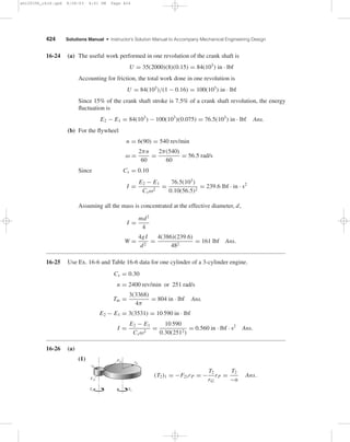
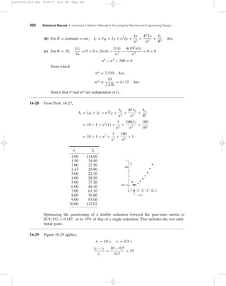
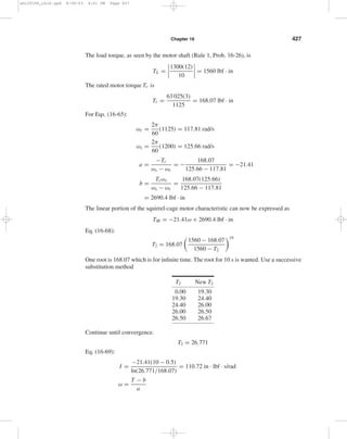
433. Chapter 17 433
Ex. 17-2: b = 10 in, d = 16 in, D = 32 in,
Polyamide A-3, t = 0.13 in, γ = 0.042, Fa =
100 lbf/in, Cp = 0.94, Cv = 1, f = 0.8
T =
63 025(60)(1.15)(1.05)
860
= 5313 lbf · in
w = 12 γ bt = 12(0.042)(10)(0.13)
= 0.655 lbf/ft
V = πdn/12 = π(16)(860/12) = 3602 ft/min
θd = 3.037 rad
For fully-developed friction:
exp( f θd) = [0.8(3.037)] = 11.35
Fc =
wV2
g
=
0.655(3602/60)2
32.174
= 73.4 lbf
(F1)a = F1 = bFaCpCv
= 10(100)(0.94)(1) = 940 lbf
F = 2T/D = 2(5313)/(16) = 664 lbf
F2 = F1 − F = 940 − 664 = 276 lbf
Fi =
F1 + F2
2
− Fc
=
940 + 276
2
− 73.4 = 535 lbf
Transmitted power H (or Ha):
H =
F(V)
33 000
=
664(3602)
33 000
= 72.5 hp
f =
1
θd
ln
F1 − Fc
F2 − Fc
=
1
3.037
ln
940 − 73.4
276 − 73.4
= 0.479 undeveloped
Note, in this as well as in the double-size case,
exp( f θd) is not used. It will show up if we
relax Fi (and change other parameters to trans-
mit the required power), in order to bring f up
to f = 0.80, and increase belt life.
You may wish to suggest to your students
that solving comparison problems in this man-
ner assists in the design process.
Doubled: b = 20 in, d = 32 in, D = 72 in,
Polyamide A-3, t = 0.26 in, γ = 0.042,
Fa = 2(100) = 200 lbf/in, Cp = 1, Cv = 1,
f = 0.8
T = 4(5313) = 21 252 lbf · in
w = 12(0.042)(20)(0.26) = 2.62 lbf/ft
V = π(32)(860/12) = 7205 ft/min
θ = 3.037 rad
For fully-developed friction:
exp( f θd) = exp[0.8(3.037)] = 11.35
Fc =
wV2
g
=
0.262(7205/60)2
32.174
= 1174.3 lbf
(F1)a = 20(200)(1)(1)
= 4000 lbf = F1
F = 2T/D = 2(21 252)/(32) = 1328.3 lbf
F2 = F1 − F = 4000 − 1328.3 = 2671.7 lbf
Fi =
F1 + F2
2
− Fc
=
4000 + 2671.7
2
− 1174.3 = 2161.6 lbf
Transmitted power H:
H =
F(V)
33 000
=
1328.3(7205)
33 000
= 290 hp
f =
1
θd
ln
F1 − Fc
F2 − Fc
=
1
3.037
ln
4000 − 1174.3
2671.7 − 1174.3
= 0.209 undeveloped
There was a small change in Cp .
Parameter Change Parameter Change
V 2-fold F 2-fold
Fc 16-fold Fi 4-fold
F1 4.26-fold Ht 4-fold
F2 9.7-fold f 0.48-fold
Note the change in Fc !
In assigning this problem, you could outline (or solicit) the three alternatives just mentioned
and assign the one of your choice–alternative 3:
shi20396_ch17.qxd 8/28/03 3:58 PM Page 433

434. 434 Solutions Manual • Instructor’s Solution Manual to Accompany Mechanical Engineering Design
17-3
As a design task, the decision set on p. 881 is useful.
A priori decisions:
• Function: Hnom = 60 hp, n = 380 rev/min, VR = 1, C = 192 in, Ks = 1.1
• Design factor: nd = 1
• Initial tension: Catenary
• Belt material: Polyamide A-3
• Drive geometry: d = D = 48 in
• Belt thickness: t = 0.13 in
Design variable: Belt width of 6 in
Use a method of trials. Initially choose b = 6 in
V =
πdn
12
=
π(48)(380)
12
= 4775 ft/min
w = 12γ bt = 12(0.042)(6)(0.13) = 0.393 lbf/ft
Fc =
wV2
g
=
0.393(4775/60)2
32.174
= 77.4 lbf
T =
63 025(1.1)(1)(60)
380
= 10 946 lbf · in
F =
2T
d
=
2(10 946)
48
= 456.1 lbf
F1 = (F1)a = bFaCpCv = 6(100)(1)(1) = 600 lbf
F2 = F1 − F = 600 − 456.1 = 143.9 lbf
Transmitted power H
H =
F(V)
33 000
=
456.1(4775)
33 000
= 66 hp
Fi =
F1 + F2
2
− Fc =
600 + 143.9
2
− 77.4 = 294.6 lbf
f =
1
θd
ln
F1 − Fc
F2 − Fc
=
1
π
ln
600 − 77.4
143.9 − 77.4
= 0.656
L = 534.8 in, from Eq. (17-2)
Friction is not fully developed, so bmin is just a little smaller than 6 in (5.7 in). Not having
a figure of merit, we choose the most narrow belt available (6 in). We can improve the
48"
192"
shi20396_ch17.qxd 8/28/03 3:58 PM Page 434

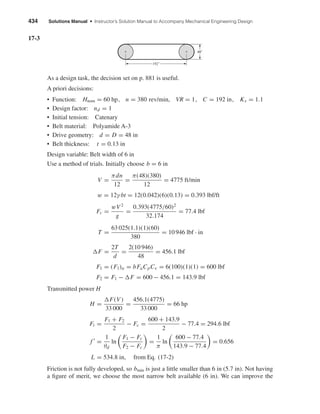
435. Chapter 17 435
design by reducing the initial tension, which reduces F1 and F2, thereby increasing belt life.
This will bring f to 0.80
F1 =
( F + Fc) exp( f θ) − Fc
exp( f θ) − 1
exp( f θ) = exp(0.80π) = 12.345
Therefore
F1 =
(456.1 + 77.4)(12.345) − 77.4
12.345 − 1
= 573.7 lbf
F2 = F1 − F = 573.7 − 456.1 = 117.6 lbf
Fi =
F1 + F2
2
− Fc =
573.7 + 117.6
2
− 77.4 = 268.3 lbf
These are small reductions since f is close to f , but improvements nevertheless.
dip =
3C2
w
2Fi
=
3(192/12)2
(0.393)
2(268.3)
= 0.562 in
17-4 From the last equation given in the Problem Statement,
exp( f φ) =
1
1 − {2T/[d(a0 − a2)b]}
1 −
2T
d(a0 − a2)b
exp( f φ) = 1
2T
d(a0 − a2)b
exp( f φ) = exp( f φ) − 1
b =
1
a0 − a2
2T
d
exp( f φ)
exp( f φ) − 1
But 2T/d = 33 000Hd/V
Thus,
b =
1
a0 − a2
33 000Hd
V
exp( f φ)
exp( f φ) − 1
Q.E.D.
17-5 Refer to Ex. 17-1 on p. 878 for the values used below.
(a) The maximum torque prior to slip is,
T =
63 025HnomKsnd
n
=
63 025(15)(1.25)(1.1)
1750
= 742.8 lbf · in Ans.
The corresponding initial tension is,
Fi =
T
D
exp( f θ) + 1
exp( f θ) − 1
=
742.8
6
11.17 + 1
11.17 − 1
= 148.1 lbf Ans.
shi20396_ch17.qxd 8/28/03 3:58 PM Page 435

436. 436 Solutions Manual • Instructor’s Solution Manual to Accompany Mechanical Engineering Design
(b) See Prob. 17-4 statement. The final relation can be written
bmin =
1
FaCpCv − (12γ t/32.174)(V/60)2
33 000Ha exp( f θ)
V[exp( f θ) − 1]
=
1
100(0.7)(1) −{[12(0.042)(0.13)]/32.174}(2749/60)2
33 000(20.6)(11.17)
2749(11.17 − 1)
= 4.13 in Ans.
This is the minimum belt width since the belt is at the point of slip. The design must
round up to an available width.
Eq. (17-1):
θd = π − 2 sin−1 D − d
2C
= π − 2 sin−1 18 − 6
2(96)
= 3.016 511 rad
θD = π + 2 sin−1 D − d
2C
= π + 2 sin−1 18 − 6
2(96)
= 3.266 674
Eq. (17-2):
L = [4(96)2
− (18 − 6)2
]1/2
+
1
2
[18(3.266 674) + 6(3.016 511)]
= 230.074 in Ans.
(c) F =
2T
d
=
2(742.8)
6
= 247.6 lbf
(F1)a = bFaCpCv = F1 = 4.13(100)(0.70)(1) = 289.1 lbf
F2 = F1 − F = 289.1 − 247.6 = 41.5 lbf
Fc = 25.6
0.271
0.393
= 17.7 lbf
Fi =
F1 + F2
2
− Fc =
289.1 + 41.5
2
− 17.7 = 147.6 lbf
Transmitted belt power H
H =
F(V)
33 000
=
247.6(2749)
33 000
= 20.6 hp
nf s =
H
HnomKs
=
20.6
15(1.25)
= 1.1
shi20396_ch17.qxd 8/28/03 3:58 PM Page 436

437. Chapter 17 437
If you only change the belt width, the parameters in the following table change as shown.
Ex. 17-1 This Problem
b 6.00 4.13
w 0.393 0.271
Fc 25.6 17.6
(F1)a 420 289
F2 172.4 42
Fi 270.6 147.7
f 0.33* 0.80**
dip 0.139 0.176
*Friction underdeveloped
**Friction fully developed
17-6 The transmitted power is the same.
n-Fold
b = 6 in b = 12 in Change
Fc 25.65 51.3 2
Fi 270.35 664.9 2.46
(F1)a 420 840 2
F2 172.4 592.4 3.44
Ha 20.62 20.62 1
nfs 1.1 1.1 1
f 0.139 0.125 0.90
dip 0.328 0.114 0.34
If we relax Fi to develop full friction ( f = 0.80) and obtain longer life, then
n-Fold
b = 6 in b = 12 in Change
Fc 25.6 51.3 2
Fi 148.1 148.1 1
F1 297.6 323.2 1.09
F2 50 75.6 1.51
f 0.80 0.80 1
dip 0.255 0.503 2
shi20396_ch17.qxd 8/28/03 3:58 PM Page 437

438. 438 Solutions Manual • Instructor’s Solution Manual to Accompany Mechanical Engineering Design
17-7
Find the resultant of F1 and F2 :
α = sin−1 D − d
2C
sin α =
D − d
2C
cos α ˙= 1 −
1
2
D − d
2C
2
Rx
= F1 cos α + F2 cos α = (F1 + F2) 1 −
1
2
D − d
2C
2
Ans.
Ry
= F1 sin α − F2 sin α = (F1 − F2)
D − d
2C
Ans.
From Ex. 17-2, d = 16 in, D = 36 in, C = 16(12) = 192 in, F1 = 940 lbf, F2 = 276 lbf
α = sin−1 36 − 16
2(192)
= 2.9855◦
Rx
= (940 + 276) 1 −
1
2
36 − 16
2(192)
2
= 1214.4 lbf
Ry
= (940 − 276)
36 − 16
2(192)
= 34.6 lbf
T = (F1 − F2)
d
2
= (940 − 276)
16
2
= 5312 lbf · in
17-8 Begin with Eq. (17-10),
F1 = Fc + Fi
2 exp( f θ)
exp( f θ) − 1
Introduce Eq. (17-9):
F1 = Fc +
T
D
exp( f θ) + 1
exp( f θ) − 1
2 exp( f θ)
exp( f θ) + 1
= Fc +
2T
D
exp( f θ)
exp( f θ) − 1
F1 = Fc + F
exp( f θ)
exp( f θ) − 1
d D
C
F1
Rx
Ry
x
y
F2
␣
␣
shi20396_ch17.qxd 8/28/03 3:58 PM Page 438

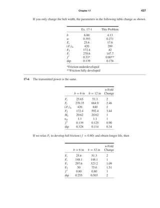
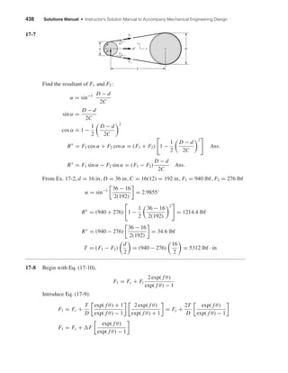
439. Chapter 17 439
Now add and subtract Fc
exp( f θ)
exp( f θ) − 1
F1 = Fc + Fc
exp( f θ)
exp( f θ) − 1
+ F
exp( f θ)
exp( f θ) − 1
− Fc
exp( f θ)
exp( f θ) − 1
F1 = (Fc + F)
exp( f θ)
exp( f θ) − 1
+ Fc − Fc
exp( f θ)
exp( f θ) − 1
F1 = (Fc + F)
exp( f θ)
exp( f θ) − 1
−
Fc
exp( f θ) − 1
F1 =
(Fc + F) exp( f θ) − Fc
exp( f θ) − 1
Q.E.D.
From Ex. 17-2: θd = 3.037 rad, F = 664 lbf, exp( f θ) = exp[0.80(3.037)] = 11.35,
and Fc = 73.4 lbf.
F1 =
(73.4 + 664)(11.35 − 73.4)
(11.35 − 1)
= 802 lbf
F2 = F1 − F = 802 − 664 = 138 lbf
Fi =
802 + 138
2
− 73.4 = 396.6 lbf
f =
1
θd
ln
F1 − Fc
F2 − Fc
=
1
3.037
ln
802 − 73.4
138 − 73.4
= 0.80 Ans.
17-9 This is a good class project. Form four groups, each with a belt to design. Once each group
agrees internally, all four should report their designs including the forces and torques on the
line shaft. If you give them the pulley locations, they could design the line shaft when they
get to Chap. 18. For now you could have the groups exchange group reports to determine
if they agree or have counter suggestions.
17-10 If you have the students implement a computer program, the design problem selections
may differ, and the students will be able to explore them. For Ks = 1.25, nd = 1.1,
d = 14 in and D = 28 in, a polyamideA-5 belt, 8 inches wide, will do(bmin = 6.58 in)
17-11 An efficiency of less than unity lowers the output for a given input. Since the object of the
drive is the output, the efficiency must be incorporated such that the belt’s capacity is in-
creased. The design power would thus be expressed as
Hd =
HnomKsnd
eff
Ans.
17-12 Some perspective on the size of Fc can be obtained from
Fc =
w
g
V
60
2
=
12γ bt
g
V
60
2
shi20396_ch17.qxd 8/28/03 3:58 PM Page 439

440. 440 Solutions Manual • Instructor’s Solution Manual to Accompany Mechanical Engineering Design
An approximate comparison of non-metal and metal belts is presented in the table
below.
Non-metal Metal
γ, lbf/in3
0.04 0.280
b, in 5.00 1.000
t, in 0.20 0.005
The ratio w/wm is
w
wm
=
12(0.04)(5)(0.2)
12(0.28)(1)(0.005)
˙= 29
The second contribution to Fc is the belt peripheral velocity which tends to be low in
metal belts used in instrument, printer, plotter and similar drives. The velocity ratio
squared influences any Fc/(Fc)m ratio.
It is common for engineers to treat Fc as negligible compared to other tensions in the
belting problem. However, when developing a computer code, one should include Fc .
17-13 Eq. (17-8):
F = F1 − F2 = (F1 − Fc)
exp( f θ) − 1
exp( f θ)
Assuming negligible centrifugal force and setting F1 = ab from step 3,
bmin =
F
a
exp( f θ)
exp( f θ) − 1
(1)
Also, Hd = HnomKsnd =
( F)V
33 000
F =
33 000HnomKsnd
V
Substituting into (1), bmin =
1
a
33 000Hd
V
exp( f θ)
exp( f θ) − 1
Ans.
17-14 The decision set for the friction metal flat-belt drive is:
A priori decisions
• Function: Hnom = 1 hp, n = 1750 rev/min, V R = 2, C ˙= 15 in, Ks = 1.2,
Np = 106
belt passes.
• Design factor: nd = 1.05
• Belt material and properties: 301/302 stainless steel
Table 17-8: Sy = 175 000 psi, E = 28 Mpsi, ν = 0.285
shi20396_ch17.qxd 8/28/03 3:58 PM Page 440

441. Chapter 17 441
• Drive geometry: d = 2 in, D = 4 in
• Belt thickness: t = 0.003 in
Design variables:
• Belt width b
• Belt loop periphery
Preliminaries
Hd = HnomKsnd = 1(1.2)(1.05) = 1.26 hp
T =
63 025(1.26)
1750
= 45.38 lbf · in
A 15 in center-to-center distance corresponds to a belt loop periphery of 39.5 in. The
40 in loop available corresponds to a 15.254 in center distance.
θd = π − 2 sin−1 4 − 2
2(15.254)
= 3.010 rad
θD = π + 2 sin−1 4 − 2
2(15.274)
= 3.273 rad
For full friction development
exp( f θd) = exp[0.35(3.010)] = 2.868
V =
πdn
12
=
π(2)(1750)
12
= 916.3 ft/s
Sy = 175 000 psi
Eq. (17-15):
Sf = 14.17(106
)(106
)−0.407
= 51 212 psi
From selection step 3
a = Sf −
Et
(1 − ν2)d
t = 51 212 −
28(106
)(0.003)
(1 − 0.2852)(2)
(0.003)
= 16.50 lbf/in of belt width
(F1)a = ab = 16.50b
For full friction development, from Prob. 17-13,
bmin =
F
a
exp( f θd)
exp( f θd) − 1
F =
2T
d
=
2(45.38)
2
= 45.38 lbf
So
bmin =
45.38
16.50
2.868
2.868 − 1
= 4.23 in
shi20396_ch17.qxd 8/28/03 3:58 PM Page 441

442. 442 Solutions Manual • Instructor’s Solution Manual to Accompany Mechanical Engineering Design
Decision #1: b = 4.5 in
F1 = (F1)a = ab = 16.5(4.5) = 74.25 lbf
F2 = F1 − F = 74.25 − 45.38 = 28.87 lbf
Fi =
F1 + F2
2
=
74.25 + 28.87
2
= 51.56 lbf
Existing friction
f =
1
θd
ln
F1
F2
=
1
3.010
ln
74.25
28.87
= 0.314
Ht =
( F)V
33 000
=
45.38(916.3)
33 000
= 1.26 hp
nf s =
Ht
HnomKs
=
1.26
1(1.2)
= 1.05
This is a non-trivial point. The methodology preserved the factor of safety corresponding
to nd = 1.1 even as we rounded bmin up to b.
Decision #2 was taken care of with the adjustment of the center-to-center distance to
accommodate the belt loop. Use Eq. (17-2) as is and solve for C to assist in this. Remem-
ber to subsequently recalculate θd and θD .
17-15 Decision set:
A priori decisions
• Function: Hnom = 5 hp, N = 1125 rev/min, V R = 3, C ˙= 20 in, Ks = 1.25,
Np = 106
belt passes
• Design factor: nd = 1.1
• Belt material: BeCu, Sy = 170 000 psi, E = 17(106
) psi, ν = 0.220
• Belt geometry: d = 3 in, D = 9 in
• Belt thickness: t = 0.003 in
Design decisions
• Belt loop periphery
• Belt width b
Preliminaries:
Hd = HnomKsnd = 5(1.25)(1.1) = 6.875 hp
T =
63 025(6.875)
1125
= 385.2 lbf · in
Decision #1: Choose a 60-in belt loop with a center-to-center distance of 20.3 in.
θd = π − 2 sin−1 9 − 3
2(20.3)
= 2.845 rad
θD = π + 2 sin−1 9 − 3
2(20.3)
= 3.438 rad
shi20396_ch17.qxd 8/28/03 3:58 PM Page 442

443. Chapter 17 443
For full friction development:
exp( f θd) = exp[0.32(2.845)] = 2.485
V =
πdn
12
=
π(3)(1125)
12
= 883.6 ft/min
Sf = 56 670 psi
From selection step 3
a = Sf −
Et
(1 − ν2)d
t = 56 670 −
17(106
)(0.003)
(1 − 0.222)(3)
(0.003) = 116.4 lbf/in
F =
2T
d
=
2(385.2)
3
= 256.8 lbf
bmin =
F
a
exp( f θd)
exp( f θd) − 1
=
256.8
116.4
2.485
2.485 − 1
= 3.69 in
Decision #2: b = 4 in
F1 = (F1)a = ab = 116.4(4) = 465.6 lbf
F2 = F1 − F = 465.6 − 256.8 = 208.8 lbf
Fi =
F1 + F2
2
=
465.6 + 208.8
2
= 337.3 lbf
Existing friction
f =
1
θd
ln
F1
F2
=
1
2.845
ln
465.6
208.8
= 0.282
H =
( F)V
33 000
=
256.8(883.6)
33 000
= 6.88 hp
nf s =
H
5(1.25)
=
6.88
5(1.25)
= 1.1
Fi can be reduced only to the point at which f = f = 0.32. From Eq. (17-9)
Fi =
T
d
exp( f θd) + 1
exp( f θd) − 1
=
385.2
3
2.485 + 1
2.485 − 1
= 301.3 lbf
Eq. (17-10):
F1 = Fi
2 exp( f θd)
exp( f θd) + 1
= 301.3
2(2.485)
2.485 + 1
= 429.7 lbf
F2 = F1 − F = 429.7 − 256.8 = 172.9 lbf
and f = f = 0.32
17-16 This solution is the result of a series of five design tasks involving different belt thick-
nesses. The results are to be compared as a matter of perspective. These design tasks are
accomplished in the same manner as in Probs. 17-14 and 17-15 solutions.
shi20396_ch17.qxd 8/28/03 3:58 PM Page 443

444. 444 Solutions Manual • Instructor’s Solution Manual to Accompany Mechanical Engineering Design
The details will not be presented here, but the table is provided as a means of learning.
Five groups of students could each be assigned a belt thickness. You can form a table from
their results or use the table below
t, in
0.002 0.003 0.005 0.008 0.010
b 4.000 3.500 4.000 1.500 1.500
CD 20.300 20.300 20.300 18.700 20.200
a 109.700 131.900 110.900 194.900 221.800
d 3.000 3.000 3.000 5.000 6.000
D 9.000 9.000 9.000 15.000 18.000
Fi 310.600 333.300 315.200 215.300 268.500
F1 439.000 461.700 443.600 292.300 332.700
F2 182.200 209.000 186.800 138.200 204.300
nf s 1.100 1.100 1.100 1.100 1.100
L 60.000 60.000 60.000 70.000 80.000
f 0.309 0.285 0.304 0.288 0.192
Fi 301.200 301.200 301.200 195.700 166.600
F1 429.600 429.600 429.600 272.700 230.800
F2 172.800 172.800 172.800 118.700 102.400
f 0.320 0.320 0.320 0.320 0.320
The first three thicknesses result in the same adjusted Fi , F1 and F2 (why?). We have no
figure of merit, but the costs of the belt and the pulleys is about the same for these three
thicknesses. Since the same power is transmitted and the belts are widening, belt forces
are lessening.
17-17 This is a design task. The decision variables would be belt length and belt section, which
could be combined into one, such as B90. The number of belts is not an issue.
We have no figure of merit, which is not practical in a text for this application. I sug-
gest you gather sheave dimensions and costs and V-belt costs from a principal vendor and
construct a figure of merit based on the costs. Here is one trial.
Preliminaries: For a single V-belt drive with Hnom = 3 hp, n = 3100 rev/min,
D = 12 in, and d = 6.2 in, choose a B90 belt, Ks = 1.3 and nd = 1.
Lp = 90 + 1.8 = 91.8 in
Eq. (17-16b):
C = 0.25



91.8 −
π
2
(12 + 6.2) + 91.8 −
π
2
(12 + 6.2)
2
− 2(12 − 6.2)2



= 31.47 in
θd = π − 2 sin−1 12 − 6.2
2(31.47)
= 2.9570 rad
exp( f θd) = exp[0.5123(2.9570)] = 4.5489
V =
πdn
12
=
π(6.2)(3100)
12
= 5031.8 ft/min
shi20396_ch17.qxd 8/28/03 3:58 PM Page 444

445. Chapter 17 445
Table 17-13:
Angle θ = θd
180°
π
= (2.957 rad)
180°
π
= 169.42°
The footnote regression equation gives K1 without interpolation:
K1 = 0.143 543 + 0.007 468(169.42°) − 0.000 015 052(169.42°)2
= 0.9767
The design power is
Hd = HnomKsnd = 3(1.3)(1) = 3.9 hp
From Table 17-14 for B90, K2 = 1. From Table 17-12 take a marginal entry of Htab = 4,
although extrapolation would give a slightly lower Htab .
Eq. (17-17): Ha = K1K2 Htab
= 0.9767(1)(4) = 3.91 hp
The allowable Fa is given by
Fa =
63 025Ha
n(d/2)
=
63 025(3.91)
3100(6.2/2)
= 25.6 lbf
The allowable torque Ta is
Ta =
Fad
2
=
25.6(6.2)
2
= 79.4 lbf · in
From Table 17-16, Kc = 0.965. Thus, Eq. (17-21) gives,
Fc = 0.965
5031.8
1000
2
= 24.4 lbf
At incipient slip, Eq. (17-9) provides:
Fi =
T
d
exp( f θ) + 1
exp( f θ) − 1
=
79.4
6.2
4.5489 + 1
4.5489 − 1
= 20.0 lbf
Eq. (17-10):
F1 = Fc + Fi
2 exp( f θ)
exp( f θ) + 1
= 24.4 + 20
2(4.5489)
4.5489 + 1
= 57.2 lbf
Thus, F2 = F1 − Fa = 57.2 − 25.6 = 31.6 lbf
Eq. (17-26): nf s =
Ha Nb
Hd
=
(3.91)(1)
3.9
= 1.003 Ans.
If we had extrapolated for Htab, the factor of safety would have been slightly less
than one.
Life Use Table 17-16 to find equivalent tensions T1 and T2 .
T1 = F1 + (Fb)1 = F1 +
Kb
d
= 57.2 +
576
6.2
= 150.1 lbf
T2 = F1 + (Fb)2 = F1 +
Kb
D
= 57.2 +
576
12
= 105.2 lbf
shi20396_ch17.qxd 8/28/03 3:58 PM Page 445

446. 446 Solutions Manual • Instructor’s Solution Manual to Accompany Mechanical Engineering Design
From Eq. (17-27), the number of belt passes is:
NP =
1193
150.1
−10.929
+
1193
105.2
−10.929 −1
= 6.76(109
)
From Eq. (17-28) for NP > 109
,
t =
NP Lp
720V
>
109
(91.8)
720(5031.8)
t > 25 340 h Ans.
Suppose nf s was too small. Compare these results with a 2-belt solution.
Htab = 4 hp/belt, Ta = 39.6 lbf · in/belt,
Fa = 12.8 lbf/belt, Ha = 3.91 hp/belt
nf s =
Nb Ha
Hd
=
Nb Ha
HnomKs
=
2(3.91)
3(1.3)
= 2.0
Also, F1 = 40.8 lbf/belt, F2 = 28.0 lbf/belt,
Fi = 9.99 lbf/belt, Fc = 24.4 lbf/belt
(Fb)1 = 92.9 lbf/belt, (Fb)2 = 48 lbf/belt
T1 = 133.7 lbf/belt, T2 = 88.8 lbf/belt
NP = 2.39(1010
) passes, t > 605 600 h
Initial tension of the drive:
(Fi )drive = Nb Fi = 2(9.99) = 20 lbf
17-18 Given: two B85 V-belts with d = 5.4 in, D = 16 in, n = 1200 rev/min, and Ks = 1.25
Table 17-11: Lp = 85 + 1.8 = 86.8 in
Eq. (17-17b):
C = 0.25



86.8 −
π
2
(16 + 5.4) + 86.8 −
π
2
(16 + 5.4)
2
− 2(16 − 5.4)2



= 26.05 in Ans.
Eq. (17-1):
θd = 180° − 2 sin−1 16 − 5.4
2(26.05)
= 156.5°
From table 17-13 footnote:
K1 = 0.143 543 + 0.007 468(156.5°) − 0.000 015 052(156.5°)2
= 0.944
Table 17-14: K2 = 1
Belt speed: V =
π(5.4)(1200)
12
= 1696 ft/min
shi20396_ch17.qxd 8/28/03 3:58 PM Page 446

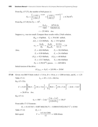
447. Chapter 17 447
Use Table 17-12 to interpolate for Htab.
Htab = 1.59 +
2.62 − 1.59
2000 − 1000
(1696 − 1000) = 2.31 hp/belt
Ha = K1K2 Nb Htab = 1(0.944)(2)(2.31) = 4.36 hp
Assuming nd = 1
Hd = Ks Hnomnd = 1.25(1)Hnom
For a factor of safety of one,
Ha = Hd
4.36 = 1.25Hnom
Hnom =
4.36
1.25
= 3.49 hp Ans.
17-19 Given: Hnom = 60 hp, n = 400 rev/min, Ks = 1.4, d = D = 26 in on 12 ft centers.
Designtask:specifyV-beltandnumberofstrands(belts).Tentativedecision:UseD360belts.
Table 17-11: Lp = 360 + 3.3 = 363.3 in
Eq. (17-16b):
C = 0.25



363.3 −
π
2
(26 + 26) + 363.3 −
π
2
(26 + 26)
2
− 2(26 − 26)2



= 140.8 in (nearly 144 in)
θd = π, θD = π, exp[0.5123π] = 5.0,
V =
πdn
12
=
π(26)(400)
12
= 2722.7 ft/min
Table 17-13: For θ = 180°, K1 = 1
Table 17-14: For D360, K2 = 1.10
Table 17-12: Htab = 16.94 hp by interpolation
Thus, Ha = K1K2 Htab = 1(1.1)(16.94) = 18.63 hp
Hd = Ks Hnom = 1.4(60) = 84 hp
Number of belts, Nb
Nb =
Ks Hnom
K1K2 Htab
=
Hd
Ha
=
84
18.63
= 4.51
Round up to five belts. It is left to the reader to repeat the above for belts such as C360
and E360.
Fa =
63 025Ha
n(d/2)
=
63 025(18.63)
400(26/2)
= 225.8 lbf/belt
Ta =
( Fa)d
2
=
225.8(26)
2
= 2935 lbf · in/belt
shi20396_ch17.qxd 8/28/03 3:58 PM Page 447

448. 448 Solutions Manual • Instructor’s Solution Manual to Accompany Mechanical Engineering Design
Eq. (17-21):
Fc = 3.498
V
1000
2
= 3.498
2722.7
1000
2
= 25.9 lbf/belt
At fully developed friction, Eq. (17-9) gives
Fi =
T
d
exp( f θ) + 1
exp( f θ) − 1
=
2935
26
5 + 1
5 − 1
= 169.3 lbf/belt
Eq. (17-10): F1 = Fc + Fi
2 exp( f θ)
exp( f θ) + 1
= 25.9 + 169.3
2(5)
5 + 1
= 308.1 lbf/belt
F2 = F1 − Fa = 308.1 − 225.8 = 82.3 lbf/belt
nf s =
Ha Nb
Hd
=
(185.63)
84
= 1.109 Ans.
Reminder: Initial tension is for the drive
(Fi )drive = Nb Fi = 5(169.3) = 846.5 lbf
A 360 belt is at the right-hand edge of the range of center-to-center pulley distances.
D ≤ C ≤ 3(D + d)
26 ≤ C ≤ 3(26 + 26)
17-20 Preliminaries: D ˙= 60 in, 14-in wide rim, Hnom = 50 hp, n = 875 rev/min, Ks = 1.2,
nd = 1.1, mG = 875/170 = 5.147, d ˙= 60/5.147 = 11.65 in
(a) From Table 17-9, an 11-in sheave exceeds C-section minimum diameter and pre-
cludes D- and E-section V-belts.
Decision: Use d = 11 in, C270 belts
Table 17-11: Lp = 270 + 2.9 = 272.9 in
C = 0.25



272.9 −
π
2
(60 + 11) + 272.9 −
π
2
(60 + 11)
2
− 2(60 − 11)2



= 76.78 in
This fits in the range
D < C < 3(D + d)
60 < C < 3(60 + 11)
60 in < C < 213 in
θd = π − 2 sin−1 60 − 11
2(76.78)
= 2.492 rad
θD = π + 2 sin−1 60 − 11
2(76.78)
= 3.791 rad
exp[0.5123(2.492)] = 3.5846
shi20396_ch17.qxd 8/28/03 3:58 PM Page 448

449. Chapter 17 449
For the flat on flywheel
exp[0.13(3.791)] = 1.637
V =
πdn
12
=
π(11)(875)
12
= 2519.8 ft/min
Table 17-13: Regression equation gives K1 = 0.90
Table 17-14: K2 = 1.15
Table 17-12: Htab = 7.83 hp/belt by interpolation
Eq. (17-17): Ha = K1K2 Htab = 0.905(1.15)(7.83) = 8.15 hp
Eq. (17-19): Hd = HnomKsnd = 50(1.2)(1.1) = 66 hp
Eq. (17-20): Nb =
Hd
Ha
=
66
8.15
= 8.1 belts
Decision: Use 9 belts. On a per belt basis,
Fa =
63 025Ha
n(d/2)
=
63 025(8.15)
875(11/2)
= 106.7 lbf/belt
Ta =
Fad
2
=
106.7(11)
2
= 586.9 lbf per belt
Fc = 1.716
V
1000
2
= 1.716
2519.8
1000
2
= 10.9 lbf/belt
At fully developed friction, Eq. (17-9) gives
Fi =
T
d
exp( f θd) + 1
exp( f θd) − 1
=
586.9
11
3.5846 + 1
3.5846 − 1
= 94.6 lbf/belt
Eq. (17-10):
F1 = Fc + Fi
2 exp( f θd)
exp( f θd) + 1
= 10.9 + 94.6
2(3.5846)
3.5846 + 1
= 158.8 lbf/belt
F2 = F1 − Fa = 158.8 − 106.7 = 52.1 lbf/belt
nf s =
Nb Ha
Hd
=
9(8.15)
66
= 1.11 O.K. Ans.
Durability:
(Fb)1 = 145.45 lbf/belt, (Fb)2 = 76.7 lbf/belt
T1 = 304.4 lbf/belt, T2 = 185.6 lbf/belt
and t > 150 000 h
Remember: (Fi )drive = 9(94.6) = 851.4 lbf
Table 17-9: C-section belts are 7/8" wide. Check sheave groove spacing to see if
14"-width is accommodating.
shi20396_ch17.qxd 8/28/03 3:58 PM Page 449

450. 450 Solutions Manual • Instructor’s Solution Manual to Accompany Mechanical Engineering Design
(b) The fully developed friction torque on the flywheel using the flats of the V-belts is
Tflat = Fi
exp( f θ) − 1
exp( f θ) + 1
= 60(94.6)
1.637 − 1
1.637 + 1
= 1371 lbf · in per belt
The flywheel torque should be
Tfly = mGTa = 5.147(586.9) = 3021 lbf · in per belt
but it is not. There are applications, however, in which it will work. For example,
make the flywheel controlling. Yes. Ans.
17-21
(a) S is the spliced-in string segment length
De is the equatorial diameter
D is the spliced string diameter
δ is the radial clearance
S + π De = π D = π(De + 2δ) = π De + 2πδ
From which
δ =
S
2π
The radial clearance is thus independent of De .
δ =
12(6)
2π
= 11.5 in Ans.
This is true whether the sphere is the earth, the moon or a marble. Thinking in terms
of a radial or diametral increment removes the basic size from the problem. Viewpoint
again!
(b) and (c)
Table 17-9: For an E210 belt, the thickness is 1 in.
dP − di =
210 + 4.5
π
−
210
π
=
4.5
π
2δ =
4.5
π
δ =
4.5
2π
= 0.716 in
0.716"
1"
dp
Dp
␦
␦
Pitch surface
60"
DЈ
S
De ␦
shi20396_ch17.qxd 8/28/03 3:58 PM Page 450

451. Chapter 17 451
The pitch diameter of the flywheel is
DP − 2δ = D
DP = D + 2δ = 60 + 2(0.716) = 61.43 in
We could make a table:
Diametral Section
Growth A B C D E
2δ
1.3
π
1.8
π
2.9
π
3.3
π
4.5
π
The velocity ratio for the D-section belt of Prob. 17-20 is
mG =
D + 2δ
d
=
60 + 3.3/π
11
= 5.55 Ans.
for the V-flat drive as compared to ma = 60/11 = 5.455 for the VV drive.
The pitch diameter of the pulley is still d = 11 in, so the new angle of wrap, θd, is
θd = π − 2 sin−1 D + 2δ − d
2C
Ans.
θD = π + 2 sin−1 D + 2δ − d
2C
Ans.
Equations (17-16a) and (17-16b) are modified as follows
Lp = 2C +
π
2
(D + 2δ + d) +
(D + δ − d)2
4C
Ans.
Cp = 0.25



Lp −
π
2
(D + 2δ + d)
+ Lp −
π
2
(D + 2δ + d)
2
− 2(D + 2δ − d)2



Ans.
The changes are small, but if you are writing a computer code for a V-flat drive,
remember that θd and θD changes are exponential.
17-22 This design task involves specifying a drive to couple an electric motor running at
1720 rev/min to a blower running at 240 rev/min, transmitting two horsepower with a
center distance of at least 22 inches. Instead of focusing on the steps, we will display two
different designs side-by-side for study. Parameters are in a “per belt” basis with per drive
quantities shown along side, where helpful.
shi20396_ch17.qxd 8/28/03 3:58 PM Page 451

452. 452 Solutions Manual • Instructor’s Solution Manual to Accompany Mechanical Engineering Design
Parameter Four A-90 Belts Two A-120 Belts
mG 7.33 7.142
Ks 1.1 1.1
nd 1.1 1.1
K1 0.877 0.869
K2 1.05 1.15
d, in 3.0 4.2
D, in 22 30
θd, rad 2.333 2.287
V, ft/min 1350.9 1891
exp( f θd) 3.304 3.2266
Lp, in 91.3 101.3
C, in 24.1 31
Htab, uncorr. 0.783 1.662
Nb Htab, uncorr. 3.13 3.326
Ta, lbf · in 26.45(105.8) 60.87(121.7)
Fa, lbf 17.6(70.4) 29.0(58)
Ha, hp 0.721(2.88) 1.667(3.33)
nf s 1.192 1.372
F1, lbf 26.28(105.2) 44(88)
F2, lbf 8.67(34.7) 15(30)
(Fb)1, lbf 73.3(293.2) 52.4(109.8)
(Fb)2, lbf 10(40) 7.33(14.7)
Fc, lbf 1.024 2.0
Fi , lbf 16.45(65.8) 27.5(55)
T1, lbf · in 99.2 96.4
T2, lbf · in 36.3 57.4
N , passes 1.61(109
) 2.3(109
)
t > h 93 869 89 080
Conclusions:
• Smaller sheaves lead to more belts.
• Larger sheaves lead to larger D and larger V.
• Larger sheaves lead to larger tabulated power.
• The discrete numbers of belts obscures some of the variation. The factors of safety
exceed the design factor by differing amounts.
17-23 In Ex. 17-5 the selected chain was 140-3, making the pitch of this 140 chain14/8 = 1.75 in.
Table 17-19 confirms.
17-24
(a) Eq. (17-32): H1 = 0.004N1.08
1 n0.9
1 p(3−0.07p)
Eq. (17-33): H2 =
1000Kr N1.5
1 p0.8
n1.5
1
shi20396_ch17.qxd 8/28/03 3:58 PM Page 452

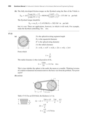
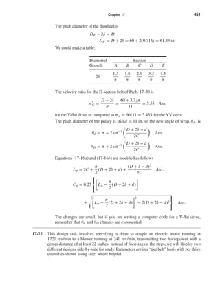
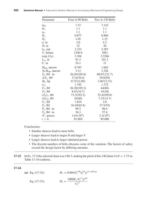
453. Chapter 17 453
Equating and solving for n1 gives
n1 =
0.25(106
)Kr N0.42
1
p(2.2−0.07p)
1/2.4
Ans.
(b) For a No. 60 chain, p = 6/8 = 0.75 in, N1 = 17, Kr = 17
n1 =
0.25(106
)(17)(17)0.42
0.75[2.2−0.07(0.75)]
1/2.4
= 1227 rev/min Ans.
Table 17-20 confirms that this point occurs at 1200 ± 200 rev/min.
(c) Life predictions using Eq. (17-40) are possible at speeds greater than 1227 rev/min.
Ans.
17-25 Given: a double strand No. 60 roller chain with p = 0.75 in, N1 = 13 teeth at 300 rev/min,
N2 = 52 teeth.
(a) Table 17-20: Htab = 6.20 hp
Table 17-22: K1 = 0.75
Table 17-23: K2 = 1.7
Use Ks = 1
Eq. (17-37):
Ha = K1K2 Htab = 0.75(1.7)(6.20) = 7.91 hp Ans.
(b) Eqs. (17-35) and (17-36) with L/p = 82
A =
13 + 52
2
− 82 = −49.5[
C =
p
4

49.5 + 49.52 − 8
52 − 13
2π
2

 = 23.95p
C = 23.95(0.75) = 17.96 in, round up to 18 in Ans.
(c) For 30 percent less power transmission,
H = 0.7(7.91) = 5.54 hp
T =
63 025(5.54)
300
= 1164 lbf · in Ans.
Eq. (17-29):
D =
0.75
sin(180◦/13)
= 3.13 in
F =
T
r
=
1164
3.13/2
= 744 lbf Ans.
shi20396_ch17.qxd 8/28/03 3:58 PM Page 453

454. 454 Solutions Manual • Instructor’s Solution Manual to Accompany Mechanical Engineering Design
17-26 Given: No. 40-4 chain, N1 = 21 teeth for n = 2000 rev/min, N2 = 84 teeth,
h = 20 000 hours.
(a) Chain pitch is p = 4/8 = 0.500 in and C ˙= 20 in.
Eq. (17-34):
L
p
=
2(20)
0.5
+
21 + 84
2
+
(84 − 21)2
4π2(20/0.5)
= 135 pitches (or links)
L = 135(0.500) = 67.5 in Ans.
(b) Table 17-20: Htab = 7.72 hp (post-extreme power)
Eq. (17-40): Since K1 is required, the N3.75
1 term is omitted.
const =
7.722.5
(15 000)
135
= 18 399
Htab =
18 399(135)
20 000
1/2.5
= 6.88 hp Ans.
(c) Table 17-22:
K1 =
21
17
1.5
= 1.37
Table 17-23: K2 = 3.3
Ha = K1K2 Htab = 1.37(3.3)(6.88) = 31.1 hp Ans.
(d) V =
N1 pn
12
=
21(0.5)(2000)
12
= 1750 ft/min
F1 =
33 000(31.1)
1750
= 586 lbf Ans.
17-27 This is our first design/selection task for chain drives. A possible decision set:
A priori decisions
• Function: Hnom, n1, space, life, Ks
• Design factor: nd
• Sprockets: Tooth counts N1 and N2, factors K1 and K2
Decision variables
• Chain number
• Strand count
• Lubrication type
• Chain length in pitches
Function: Motor with Hnom = 25 hp at n = 700 rev/min; pump at n = 140 rev/min;
mG = 700/140 = 5
Design Factor: nd = 1.1
Sprockets: Tooth count N2 = mG N1 = 5(17) = 85 teeth–odd and unavailable. Choose
84 teeth. Decision: N1 = 17, N2 = 84
shi20396_ch17.qxd 8/28/03 3:58 PM Page 454

455. Chapter 17 455
Evaluate K1 and K2
Eq. (17-38): Hd = HnomKsnd
Eq. (17-37): Ha = K1K2 Htab
Equate Hd to Ha and solve for Htab :
Htab =
Ksnd Hnom
K1K2
Table 17-22: K1 = 1
Table 17-23: K2 = 1, 1.7, 2.5, 3.3 for 1 through 4 strands
Htab =
1.5(1.1)(25)
(1)K2
=
41.25
K2
Prepare a table to help with the design decisions:
Chain Lub.
Strands K2 Htab No. Htab nf s Type
1 1.0 41.3 100 59.4 1.58 B
2 1.7 24.3 80 31.0 1.40 B
3 2.5 16.5 80 31.0 2.07 B
4 3.3 12.5 60 13.3 1.17 B
Design Decisions
We need a figure of merit to help with the choice. If the best was 4 strands of No. 60
chain, then
Decision #1 and #2: Choose four strand No. 60 roller chain with nf s = 1.17.
nf s =
K1K2 Htab
Ks Hnom
=
1(3.3)(13.3)
1.5(25)
= 1.17
Decision #3: Choose Type B lubrication
Analysis:
Table 17-20: Htab = 13.3 hp
Table 17-19: p = 0.75 in
Try C = 30 in in Eq. (17-34):
L
p
=
2C
p
+
N1 + N2
2
+
(N2 − N1)2
4π2C/p
= 2(30/0.75) +
17 + 84
2
+
(84 − 17)2
4π2(30/0.75)
= 133.3 → 134
From Eq. (17-35) with p = 0.75 in,C = 30.26 in.
Decision #4: Choose C = 30.26 in.
shi20396_ch17.qxd 8/28/03 3:58 PM Page 455

456. 456 Solutions Manual • Instructor’s Solution Manual to Accompany Mechanical Engineering Design
17-28 Follow the decision set outlined in Prob. 17-27 solution. We will form two tables, the first
for a 15 000 h life goal, and a second for a 50 000 h life goal. The comparison is useful.
Function: Hnom = 50 hp at n = 1800 rev/min, npump = 900 rev/min
mG = 1800/900 = 2, Ks = 1.2
life = 15 000 h, then repeat with life = 50 000 h
Design factor: nd = 1.1
Sprockets: N1 = 19 teeth, N2 = 38 teeth
Table 17-22 (post extreme):
K1 =
N1
17
1.5
=
19
17
1.5
= 1.18
Table 17-23:
K2 = 1, 1.7, 2.5, 3.3, 3.9, 4.6, 6.0
Decision variables for 15 000 h life goal:
Htab =
Ksnd Hnom
K1K2
=
1.2(1.1)(50)
1.18K2
=
55.9
K2
(1)
nf s =
K1K2 Htab
Ks Hnom
=
1.18K2 Htab
1.2(50)
= 0.0197K2 Htab
Form a table for a 15 000 h life goal using these equations.
K2 Htab Chain # Htab nf s Lub
1 1.0 55.90 120 21.6 0.423 C
2 1.7 32.90 120 21.6 0.923 C
3 2.5 22.40 120 21.6 1.064 C
4 3.3 16.90 120 21.6 1.404 C
5 3.9 14.30 80 15.6 1.106 C
6 4.6 12.20 60 12.4 1.126 C
8 6.0 9.32 60 12.4 1.416 C
There are 4 possibilities where nf s ≥ 1.1
Decision variables for 50 000h life goal
From Eq. (17-40), the power-life tradeoff is:
(Htab)2.5
15 000 = (Htab)2.5
50 000
Htab =
15 000
50 000
(Htab)2.5
1/2.5
= 0.618 Htab
Substituting from (1),
Htab = 0.618
55.9
K2
=
34.5
K2
shi20396_ch17.qxd 8/28/03 3:58 PM Page 456

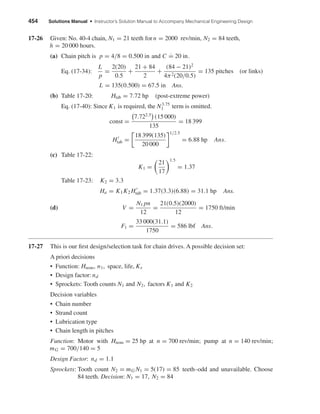
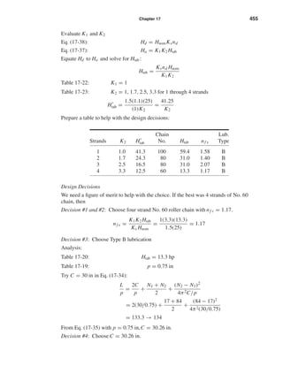
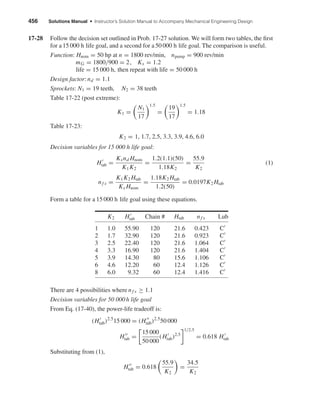
457. Chapter 17 457
The H notation is only necessary because we constructed the first table, which we nor-
mally would not do.
nf s =
K1K2 Htab
Ks Hnom
=
K1K2(0.618Htab)
Ks Hnom
= 0.618[(0.0197)K2 Htab] = 0.0122K2 Htab
Form a table for a 50 000 h life goal.
K2 Htab Chain # Htab nf s Lub
1 1.0 34.50 120 21.6 0.264 C
2 1.7 20.30 120 21.6 0.448 C
3 2.5 13.80 120 21.6 0.656 C
4 3.3 10.50 120 21.6 0.870 C
5 3.9 8.85 120 21.6 1.028 C
6 4.6 7.60 120 21.6 1.210 C
8 6.0 5.80 80 15.6 1.140 C
There are two possibilities in the second table with nf s ≥ 1.1. (The tables allow for the
identification of a longer life one of the outcomes.) We need a figure of merit to help with
the choice; costs of sprockets and chains are thus needed, but is more information than
we have.
Decision #1: #80 Chain (smaller installation) Ans.
nf s = 0.0122K2 Htab = 0.0122(8.0)(15.6) = 1.14 O.K.
Decision #2: 8-Strand, No. 80 Ans.
Decision #3: Type C Lubrication Ans.
Decision #4: p = 1.0 in, C is in midrange of 40 pitches
L
p
=
2C
p
+
N1 + N2
2
+
(N2 − N1)2
4π2C/p
= 2(40) +
19 + 38
2
+
(38 − 19)2
4π2(40)
= 108.7 ⇒ 110 even integer Ans.
Eq. (17-36):
A =
N1 + N2
2
−
L
p
=
19 + 38
2
− 110 = −81.5
Eq. (17-35):
C
p
=
1
4

81.5 + 81.52 − 8
38 − 19
2π
2

 = 40.64
C = p(C/p) = 1.0(40.64) = 40.64 in (for reference) Ans.
shi20396_ch17.qxd 8/28/03 3:58 PM Page 457

458. 458 Solutions Manual • Instructor’s Solution Manual to Accompany Mechanical Engineering Design
17-29 The objective of the problem is to explore factors of safety in wire rope. We will express
strengths as tensions.
(a) Monitor steel 2-in 6 × 19 rope, 480 ft long
Table 17-2: Minimum diameter of a sheave is 30d = 30(2) = 60 in, preferably
45(2) = 90 in. The hoist abuses the wire when it is bent around a sheave. Table 17-24
gives the nominal tensile strength as 106 kpsi. The ultimate load is
Fu = (Su)nom Anom = 106
π(2)2
4
= 333 kip Ans.
The tensile loading of the wire is given by Eq. (17-46)
Ft =
W
m
+ wl 1 +
a
g
W = 4(2) = 8 kip, m = 1
Table (17-24):
wl = 1.60d2
l = 1.60(22
)(480) = 3072 lbf or 3.072 kip
Therefore,
Ft = (8 + 3.072) 1 +
2
32.2
= 11.76 kip Ans.
Eq. (17-48):
Fb =
Er dw Am
D
and for the 72-in drum
Fb =
12(106
)(2/13)(0.38)(22
)(10−3
)
72
= 39 kip Ans.
For use in Eq. (17-44), from Fig. 17-21
( p/Su) = 0.0014
Su = 240 kpsi, p. 908
Ff =
0.0014(240)(2)(72)
2
= 24.2 kip Ans.
(b) Factors of safety
Static, no bending:
n =
Fu
Ft
=
333
11.76
= 28.3 Ans.
Static, with bending:
Eq. (17-49): ns =
Fu − Fb
Ft
=
333 − 39
11.76
= 25.0 Ans.
shi20396_ch17.qxd 8/28/03 3:58 PM Page 458

459. Chapter 17 459
Fatigue without bending:
nf =
Ff
Ft
=
24.2
11.76
= 2.06 Ans.
Fatigue, with bending: For a life of 0.1(106
) cycles, from Fig. 17-21
( p/Su) = 4/1000 = 0.004
Ff =
0.004(240)(2)(72)
2
= 69.1 kip
Eq. (17-50): nf =
69.1 − 39
11.76
= 2.56 Ans.
If we were to use the endurance strength at 106
cycles (Ff = 24.2 kip) the factor of
safety would be less than 1 indicating 106
cycle life impossible.
Comments:
• There are a number of factors of safety used in wire rope analysis. They are differ-
ent, with different meanings. There is no substitute for knowing exactly which fac-
tor of safety is written or spoken.
• Static performance of a rope in tension is impressive.
• In this problem, at the drum, we have a finite life.
• The remedy for fatigue is the use of smaller diameter ropes, with multiple ropes
supporting the load. See Ex. 17-6 for the effectiveness of this approach. It will also
be used in Prob. 17-30.
• Remind students that wire ropes do not fail suddenly due to fatigue. The outer
wires gradually show wear and breaks; such ropes should be retired. Periodic in-
spections prevent fatigue failures by parting of the rope.
17-30 Since this is a design task, a decision set is useful.
A priori decisions
• Function: load, height, acceleration, velocity, life goal
• Design Factor: nd
• Material: IPS, PS, MPS or other
• Rope: Lay, number of strands, number of wires per strand
Decision variables:
• Nominal wire size: d
• Number of load-supporting wires: m
From experience with Prob. 17-29, a 1-in diameter rope is not likely to have much of a
life, so approach the problem with the d and m decisions open.
Function: 5000 lbf load, 90 foot lift,acceleration = 4 ft/s2
,velocity = 2 ft/s, life
goal = 105
cycles
Design Factor: nd = 2
Material: IPS
Rope: Regular lay, 1-in plow-steel 6 × 19 hoisting
shi20396_ch17.qxd 8/28/03 3:58 PM Page 459

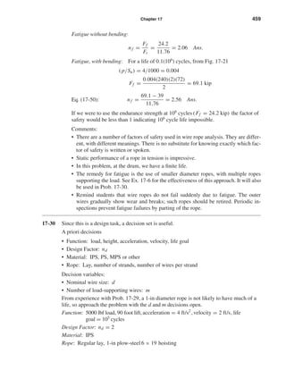
460. 460 Solutions Manual • Instructor’s Solution Manual to Accompany Mechanical Engineering Design
Design variables
Choose 30-in Dmin. Table 17-27: w = 1.60d2
lbf/ft
wl = 1.60d2
l = 1.60d2
(90) = 144d2
lbf, ea.
Eq. (17-46):
Ft =
W
m
+ wl 1 +
a
g
=
5000
m
+ 144d2
1 +
4
32.2
=
5620
m
+ 162d2
lbf, each wire
Eq. (17-47):
Ff =
( p/Su)Su Dd
2
From Fig. 17-21 for 105
cycles, p/Su = 0.004; from p. 908, Su = 240 000 psi, based on
metal area.
Ff =
0.004(240 000)(30d)
2
= 14 400d lbf each wire
Eq. (17-48) and Table 17-27:
Fb =
Ewdw Am
D
=
12(106
)(0.067d)(0.4d2
)
30
= 10 720d3
lbf, each wire
Eq. (17-45):
nf =
Ff − Fb
Ft
=
14 400d − 10 720d3
(5620/m) + 162d2
We could use a computer program to build a table similar to that of Ex. 17-6. Alterna-
tively, we could recognize that 162d2
is small compared to 5620/m, and therefore elimi-
nate the 162d2
term.
nf ˙=
14 400d − 10 720d3
5620/m
=
m
5620
(14 400d − 10 720d3
)
Maximize nf ,
∂nf
∂d
= 0 =
m
5620
[14 400 − 3(10 720)d2
]
From which
d* =
14 400
32 160
= 0.669 in
Back-substituting
nf =
m
5620
[14 400(0.669) − 10 720(0.6693
)] = 1.14 m
Thus nf =1.14, 2.28, 3.42, 4.56 for m =1, 2, 3, 4 respectively. If we choose d =0.50 in,
then m = 2.
nf =
14 400(0.5) − 10 720(0.53
)
(5620/2) + 162(0.5)2
= 2.06
shi20396_ch17.qxd 8/28/03 3:58 PM Page 460

461. Chapter 17 461
This exceeds nd = 2
Decision #1: d = 1/2 in
Decision #2: m = 2 ropes supporting load. Rope should be inspected weekly for any
signs of fatigue (broken outer wires).
Comment: Table 17-25 gives n for freight elevators in terms of velocity.
Fu = (Su)nom Anom = 106 000
πd2
4
= 83 252d2
lbf, each wire
n =
Fu
Ft
=
83 452(0.5)2
(5620/2) + 162(0.5)2
= 7.32
By comparison, interpolation for 120 ft/min gives 7.08-close. The category of construc-
tion hoists is not addressed in Table 17-25. We should investigate this before proceeding
further.
17-31 2000 ft lift, 72 in drum, 6 × 19 MS rope. Cage and load 8000 lbf, acceleration = 2 ft/s2
.
(a) Table 17-24: (Su)nom = 106 kpsi; Su = 240 kpsi (p. 1093, metal area); Fig. 17-22:
( p/Su)106 = 0.0014
Ff =
0.0014(240)(72)d
2
= 12.1d kip
Table 17-24: wl = 1.6d2
2000(10−3
) = 3.2d2
kip
Eq. (17-46): Ft = (W + wl) 1 +
a
g
= (8 + 3.2d2
) 1 +
2
32.2
= 8.5 + 3.4d2
kip
Note that bending is not included.
n =
Ff
Ft
=
12.1d
8.5 + 3.4d2
← maximum n Ans.
d, in n
0.500 0.650
1.000 1.020
1.500 1.124
1.625 1.125
1.750 1.120
2.000 1.095
shi20396_ch17.qxd 8/28/03 3:58 PM Page 461

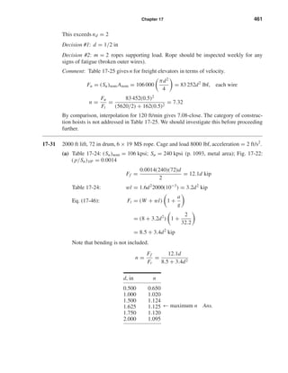
462. 462 Solutions Manual • Instructor’s Solution Manual to Accompany Mechanical Engineering Design
(b) Try m = 4 strands
Ft =
8
4
+ 3.2d2
1 +
2
32.2
= 2.12 + 3.4d2
kip
Ff = 12.1d kip
n =
12.1d
2.12 + 3.4d2
Comparing tables, multiple ropes supporting the load increases the factor of safety,
and reduces the corresponding wire rope diameter, a useful perspective.
17-32
n =
ad
b/m + cd2
dn
dd
=
(b/m + cd2
)a − ad(2cd)
(b/m + cd2)2
= 0
From which
d* =
b
mc
Ans.
n* =
a
√
b/(mc)
(b/m) + c[b/(mc)]
=
a
2
m
bc
Ans.
These results agree closely with Prob. 17-31 solution. The small differences are due to
rounding in Prob. 17-31.
17-33 From Prob. 17-32 solution:
n1 =
ad
b/m + cd2
Solve the above equation for m
m =
b
ad/n1 − cd2
(1)
dm
ad
= 0 =
[(ad/n1) − ad2
](0) − b[(a/n1) − 2cd]
[(ad/n1) − cd2]2
← maximum n Ans.
d, in n
0.5000 2.037
0.5625 2.130
0.6250 2.193
0.7500 2.250
0.8750 2.242
1.0000 2.192
shi20396_ch17.qxd 8/28/03 3:58 PM Page 462

463. Chapter 17 463
From which d* =
a
2cn1
Ans.
Substituting this result for d in Eq. (1) gives
m* =
4bcn1
a2
Ans.
17-34
Am = 0.40d2
= 0.40(22
) = 1.6 in2
Er = 12 Mpsi, w = 1.6d2
= 1.6(22
) = 6.4 lbf/ft
wl = 6.4(480) = 3072 lbf
Treat the rest of the system as rigid, so that all of the stretch is due to the cage weighing
1000 lbf and the wire’s weight. From Prob. 5-6
δ1 =
Pl
AE
+
(wl)l
2AE
=
1000(480)(12)
1.6(12)(106)
+
3072(480)(12)
2(1.6)(12)(106)
= 0.3 + 0.461 = 0.761 in
due to cage and wire. The stretch due to the wire, the cart and the cage is
δ2 =
9000(480)(12)
1.6(12)(106)
+ 0.761 = 3.461 in Ans.
17-35 to 17-38 Computer programs will vary.
shi20396_ch17.qxd 8/28/03 3:58 PM Page 463

464. Chapter 18
Comment: This chapter, when taught immediately after Chapter 7, has the advantage of im-
mediately applying the fatigue information acquired in Chapter 7. We have often done it
ourselves. However, the disadvantage is that many of the items attached to the shaft have
to be explained sufficiently so that the influence on the shaft is understood. It is the in-
structor’s call as to the best way to achieve course objectives.
This chapter is a nice note upon which to finish a study of machine elements. A very
popular first design task in the capstone design course is the design of a speed-reducer, in
which shafts, and many other elements, interplay.
18-1 The first objective of the problem is to move from shaft attachments to influences on the
shaft. The second objective is to “see” the diameter of a uniform shaft that will satisfy de-
flection and distortion constraints.
(a)
dP + (80/16)dP
2
= 12 in
dP = 4.000 in
Wt
=
63 025(50)
1200(4/2)
= 1313 lbf
Wr
= Wt
tan 25° = 1313 tan 25° = 612 lbf
W =
Wt
cos 25°
=
1313
cos 25°
= 1449 lbf
T = Wt
(d/2) = 1313(4/2) = 2626 lbf · in
Reactions RA, RB, and load W are all in the same plane.
RA = 1449(2/11) = 263 lbf
RB = 1449(9/11) = 1186 lbf
Mmax = RA(9) = 1449(2/11)(9)
= 2371 lbf · in Ans.
2"
9"
Components in xyz
238.7
111.3
A
B
z
x
y
1074.3612
1313
500.7
M
O
Mmax ϭ 2371 lbf•in
9"0 11"
11"
9" 2"
w
RA RB
shi20396_ch18.qxd 8/28/03 4:16 PM Page 464

465. Chapter 18 465
(b) Using nd = 2 and Eq. (18-1)
dA =
32nd Fb(b2
− l2
)
3π Elθall
1/4
=
32(2)(1449)(2)(22
− 112
)
3π(30)(106)(11)(0.001)
1/4
= 1.625 in
A design factor of 2 means that the slope goal is 0.001/2 or 0.0005. Eq. (18-2):
dB =
32nd Fa(l2
− a2
)
3π Elθall
1/4
=
32(2)(1449)(9)(112
− 92
)
3π(30)(106)(11)(0.001)
1/4
= 1.810 in
The diameter of a uniform shaft should equal or exceed 1.810 in. Ans.
18-2 This will be solved using a deterministic approach with nd = 2. However, the reader may
wish to explore the stochastic approach given in Sec. 7-17.
Table A-20: Sut = 68 kpsi and Sy = 37.5 kpsi
Eq. (7-8): Se = 0.504(68) = 34.27 kpsi
Eq. (7-18): ka = 2.70(68)−0.265
= 0.883
Assume a shaft diameter of 1.8 in.
Eq. (7-19): kb =
1.8
0.30
−0.107
= 0.826
kc = kd = kf = 1
From Table 7-7 for R = 0.999, ke = 0.753.
Eq. (7-17): Se = 0.883(0.826)(1)(1)(1)(0.753)(34.27) = 18.8 kpsi
From p. 444, Kt = 2.14, Kts = 2.62
With r = 0.02 in, Figs. 7-20 and 7-21 give q = 0.60 and qs = 0.77, respectively.
Eq. (7-31): Kf = 1 + 0.60(2.14 − 1) = 1.68
Kf s = 1 + 0.77(2.62 − 1) = 2.25
(a) DE-elliptic from Eq. (18-21),
d =



16(2)
π
4
1.68(2371)
18 800
2
+ 3
2.25(2626)
37 500
2 1/2



1/3
= 1.725 in Ans.
shi20396_ch18.qxd 8/28/03 4:16 PM Page 465

466. 466 Solutions Manual • Instructor’s Solution Manual to Accompany Mechanical Engineering Design
(b) DE-Gerber from Eq. (18-16),
d =

16(2)(1.68)(2371)
π(18 800)



1 + 1 + 3
2.25(2626)(18 800)
1.68(2371)(68 000)
2 1/2





1/3
= 1.687 in Ans.
From Prob. 18-1, deflection controls d = 1.81 in
18-3 It is useful to provide a cylindrical roller bearing as the heavily-loaded bearing and a ball
bearing at the other end to control the axial float, so that the roller grooves are not subject
to thrust hunting. Profile keyways capture their key. A small shoulder can locate the pinion,
and a shaft collar (or a light press fit) can capture the pinion. The key transmits the torque
in either case. The student should:
• select rolling contact bearings so that the shoulder and fillet can be sized to the bearings;
• build on the understanding gained from Probs. 18-1 and 18-2.
Each design will differ in detail so no solution is presented here.
18-4 One could take pains to model this shaft exactly, using say finite element software.
However, for the bearings and the gear, the shaft is basically of uniform diameter, 1.875 in.
The reductions in diameter at the bearings will change the results insignificantly. Use
E = 30(106
) psi.
To the left of the load:
θAB =
Fb
6E Il
(3x2
+ b2
− l2
)
=
1449(2)(3x2
+ 22
− 112
)
6(30)(106)(π/64)(1.8254)(11)
= 2.4124(10−6
)(3x2
− 117)
At x = 0: θ = −2.823(10−4
) rad
At x = 9 in: θ = 3.040(10−4
) rad
At x = 11 in: θ =
1449(9)(112
− 92
)
6(30)(106)(π/64)(1.8754)(11)
= 4.342(10−4
) rad
Left bearing: Station 1
nf s =
Allowable slope
Actual slope
=
0.001
0.000 282 3
= 3.54
Right bearing: Station 5
nf s =
0.001
0.000 434 2
= 2.30
shi20396_ch18.qxd 8/28/03 4:16 PM Page 466

467. Chapter 18 467
Gear mesh slope:
Section 18-2, p. 927, recommends a relative slope of 0.0005. While we don’t know the slope
on the next shaft, we know that it will need to have a larger diameter and be stiffer. At the
moment we can say
nf s <
0.0005
0.000 304
= 1.64
Since this is the controlling location on the shaft for distortion, nf s may be much less than
1.64.
All is not lost because crowning of teeth can relieve the slope constraint. If this is not
an option, then use Eq. (18-4) with a design factor of say 2.
dnew = dold
n(dy/dx)old
(slope)all
1/4
= 1.875
2(0.000 304)
0.000 25
1/4
= 2.341 in
Technically, all diameters should be increased by a factor of 2.341/1.875, or about 1.25.
However the bearing seat diameters cannot easily be increased and the overhang diameter
need not increase because it is straight. The shape of the neutral surface is largely controlled
by the diameter between bearings.
The shaft is unsatisfactory in distortion as indicated by the slope at the gear seat. We
leave the problem here.
18-5 Use the distortion-energy elliptic failure locus. The torque and moment loadings on the
shaft are shown below.
Candidate critical locations for strength:
• Pinion seat keyway
• Right bearing shoulder
• Coupling keyway
Preliminaries: ANSI/ASME shafting design standard uses notch sensitivities to estimate
Kf and Kf s .
Table A-20 for 1030 HR: Sut = 68 kpsi, Sy = 37.5 kpsi, HB = 137
Eq. (7-8): Se = 0.504(68) = 34.27 kpsi
Eq. (7-18): ka = 2.70(68)−0.265
= 0.883
kc = kd = ke = 1
Pinion seat keyway
See p. 444 for keyway stress concentration factors
Kt = 2.14
Kts = 2.62
Profile keyway
Moment
M, T
(lbf•in)
x
2371
2626
Torque
shi20396_ch18.qxd 8/28/03 4:16 PM Page 467

468. 468 Solutions Manual • Instructor’s Solution Manual to Accompany Mechanical Engineering Design
For an end-mill profile keyway cutter of 0.010 in radius,
From Fig. 7-20: q = 0.50
From Fig. 7-21: qs = 0.65
Eq. (7-31):
Kf s = 1 + qs(Kts − 1)
= 1 + 0.65(2.62 − 1) = 2.05
Kf = 1 + 0.50(2.14 − 1) = 1.57
Eq. (18-15):
Eq. (7-19):
A = 2Kf Ma = 2(1.57)(2371) = 7445 lbf · in
B =
√
3Kf sTm =
√
3(2.05)(2626) = 9324 lbf · in
r =
σa
σm
=
A
B
=
7445
9324
= 0.798
kb =
1.875
0.30
−0.107
= 0.822
Eq. (7-17): Se = 0.883(0.822)(0.753)(34.27) = 18.7 kpsi
Eq. (18-22):
1
n
=
16
π(1.8753)
4
1.57(2371)
18 700
2
+ 3
2.05(2626)
37 500
2 1/2
= 0.363, from which n = 2.76
Table 7-11:
Sa =
(0.798)2(37.5)2(18.7)2
(0.798)2(37.5)2 + 18.72
= 15.9 kpsi
Sm =
Sa
r
=
15.9
0.798
= 19.9 kpsi
rcrit =
15.9
37.5 − 15.9
= 0.736 < 0.7
Therefore, the threat lies in fatigue.
Right-hand bearing shoulder
The text does not give minimum and maximum shoulder diameters for 03-series bearings
(roller). Use D = 1.75 in.
r
d
=
0.030
1.574
= 0.019,
D
d
=
1.75
1.574
= 1.11
From Fig. A-15-9,
Kt = 2.4
From Fig. A-15-8,
Kts = 1.6
shi20396_ch18.qxd 8/28/03 4:16 PM Page 468

469. Chapter 18 469
From Fig. 7-20, q = 0.65
From Fig. 7-21, qs = 0.83
Kf = 1 + 0.65(2.4 − 1) = 1.91
Kf s = 1 + 0.83(1.6 − 1) = 1.50
M = 2371
0.453
2
= 537 lbf · in
Eq. (18-22):
1
n
=
16
π(1.5743)
4
1.91(537)
18 700
2
+ 3
1.50(262)
37 500
2 1/2
= 0.277, from which n = 3.61
Overhanging coupling keyway
There is no bending moment, thus Eq. (18-22) reduces to:
1
n
=
16
√
3Kf sTm
πd3Sy
=
16
√
3(1.50)(2626)
π(1.53)(37 500)
= 0.275 from which n = 3.64
Summary of safety factors:
Location nf s Solution Source
Pinion seat 2.76 Prob. 18-5
RH BRG shoulder 3.61 Prob. 18-5
Coupling keyway 3.64 Prob. 18-5
Bearing slope 2.30 Prob. 18-4
Mesh slope <1.64 Prob. 18-4
18-6 If you have assigned Probs. 18-1 through 18-5, offered suggestions, and discussed their
work, you have provided a good experience for them.
Since they are performing adequacy assessments of individual designs for this prob-
lem, each will be different. Thus no solution can be offered here.
18-7 Preliminaries:
nc = 1200
16
80
20
60
= 80 rev/min
T = 63 025
50
80
= 39 391 lbf · in
d + (20/60)d
2
= 16 in, d = 24 in
shi20396_ch18.qxd 8/28/03 4:16 PM Page 469

470. 470 Solutions Manual • Instructor’s Solution Manual to Accompany Mechanical Engineering Design
Wt
=
T
d/2
=
39 391
12
= 3283 lbf
Wr
= 3283 tan 25° = 1531 lbf
W =
Wt
cos 25°
=
3283
cos 25°
= 3622 lbf
Loads W, R1 and R2 are all in the same plane.
R1 = 3622
8
11
= 2634 lbf
R2 = 3622
3
11
= 988 lbf
The steepest slope will be at the left bearing.
Eq. (18-1):
d =
32nd Fb(b2 − l2)
3π Elθall
1/4
=
32(2)(3622)(8)(82 − 112)
3π(30)(106)(11)(0.001)
1/4
= 2.414 in
The design should proceed in the same manner as Probs. 18-1 to 18-6.
18-8 From the shaft forces in Probs. 18-1 and 18-7 solutions, we can construct the force portions
of the free-body diagram for shaft b of Fig. P18-1.
T = 63 025
50
240
= 13 130 lbf · in
3"
6"
2"
875
2276
1531
612
395 657
1313
z
y
x
3283
3"
8"
2387.6
417.5
895.43283
Components
1113.5
1531
8"
3622
R1 R2
3"
shi20396_ch18.qxd 8/28/03 4:16 PM Page 470

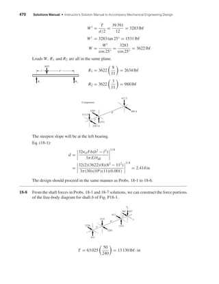
471. Chapter 18 471
The resulting forces at each location are not in the same plane; therefore, we must work in
terms of components.
The slope at the left support is the greatest.
d =
32(2)
3π(30)(106)(11)(0.001)
[1531(8)(82
− 112
) − 1313(2)(22
− 112
)]2
+ [3283(8)(82
− 112
) − 612(2)(22
− 112
)]2 1/2
1/4
= 2.320 in
with d = 2.320, determine the slopes at C, G, H, and D.
θC =
1
6(30)(106)(π/64)(2.3204)(11)
[1531(8)(82
− 112
) − 1313(2)(22
− 112
)]2
+ [3283(8)(82
− 112
) − 612(2)(22
− 112
)]2 1/2
= 0.000 500 rad (checks)
θG =
1
6(30)(106)(π/64)(2.3204)(11)
[1531(8)(3(32
) + 82
− 112
)
− 1313(2)(3(32
) + 22
− 112
)]2
+ [3283(8)(3(32
) + 82
− 112
)
− 612(2)(3(32
) + 22
− 112
)]2 1/2
= 0.000 245 rad
θH =
1
6(30)(106)(π/64)(2.3204)(11)
[1531(3)(112
− 3(22
) − 32
)
− 1313(9)(112
− 3(22
) − 92
)]2
+ [3283(3)(112
− 3(22
) − 32
)
− 612(9)(112
− 3(22
) − 92
)]2 1/2
= 0.000 298 rad
θD =
1
6(30)(106)(π/64)(2.3204)(11)
[1531(3)(112
− 32
) − 1313(9)(112
− 92
)]2
+ [3283(3)(112
− 32
) − 612(9)(112
− 92
)]2 1/2
= 0.000 314 rad
The shaft diameter should be increased for the same reason given in Problem 18-4 (gear
mesh slope).
dnew = 2.32
2(0.000 298)
0.000 25
1/4
= 2.883 in
3"
2276 612 395
3283
Horizontal plane
x
2"
C
G
DH
z
3"
875 1313
1531 657
2"
z
C
G D
H
Vertical plane
y
shi20396_ch18.qxd 8/28/03 4:16 PM Page 471

472. 472 Solutions Manual • Instructor’s Solution Manual to Accompany Mechanical Engineering Design
Strength constraints
MG = 3 8752 + 22762 = 7315 lbf · in
MH = 2 6572 + 3952 = 1533 lbf · in
Point G is more critical. Assume d = 2.88 in.
Similar to Prob. 8-2, Sut = 68 kpsi, Sy = 37.5 kpsi and ka = 0.883
Eq. (7-19): kb = 0.91(2.88)−0.157
= 0.771
kc = kd = kf = 1
For R = 0.995, Table A-10 provides z = 2.576.
Eq. (7-28): ke = 1 − 0.08(2.576) = 0.794
Eq. (7-17): Se = 0.883(0.771)(1)(1)(0.794)(1)(0.504)(68) = 18.5 kpsi
Eq. (7-31): Kf = 1.68, Kf s = 2.25
Using DE-elliptic theory, Eq. (18-21)
d =



16(2)
π
4
1.68(7315)
18 500
2
+ 3
2.25(13 130)
37 500
2 1/2



1/3
= 2.687 in O.K.
Students will approach the design differently from this point on.
18-9 The bearing ensemble reliability is related to the six individual reliabilities by
R = R1 R2 R3 R4 R5 R6
For an ensemble reliability of R,the individual reliability goals are
Ri = R1/6
The radial loads at bearings A through F were found to be
A B C D E F
263 1186 2438 767 2634 988 lbf
It may be useful to make the bearings at A, D, and F one size and those at B, C, and E an-
other size, to minimize the number of different parts. In such a case
R1 = RB RC RE, R2 = RA RD RF
R = R1 R2 = (RB RC RE)(RA RD RF)
where the reliabilities RA through RF are the reliabilities of Sec. 11-10, Eqs. (11-18),
(11-19), (11-20), and (11-21).
A corollary to the bearing reliability description exists and is given as
R = Ra Rb Rc
In this case you can begin with
Ri = R1/3
shi20396_ch18.qxd 8/28/03 4:16 PM Page 472

473. Chapter 18 473
18-10 This problem is not the same as Prob. 11-9, although the figure is the same. We have a
design task of identifying bending moment and torsion diagrams which are preliminary to
an industrial roller shaft design.
F
y
C = 30(8) = 240 lbf
Fz
C = 0.4(240) = 96 lbf
T = Fz
C(2) = 96(2) = 192 lbf · in
Fz
B =
T
1.5
=
192
1.5
= 128 lbf
F
y
B = Fz
B tan 20° = 128 tan 20° = 46.6 lbf
(a) xy-plane
MO = 240(5.75) − F
y
A(11.5) − 46.6(14.25) = 0
F
y
A =
240(5.75) − 46.6(14.25)
11.5
= 62.3 lbf
MA = F
y
O(11.5) − 46.6(2.75) − 240(5.75) = 0
F
y
O =
240(5.75) + 46.6(2.75)
11.5
= 131.1 lbf
Bending moment diagram
C
O
Ϫ754
Ϫ128
A B
Mxy
(lbf•in)
x
11.5"
5.75" AC
O
FA
y
FO
y
B
x
y
2.75"
240
46.6
z
y
Fy
B
Fz
B
Fz
C
F
y
C
shi20396_ch18.qxd 8/28/03 4:17 PM Page 473

474. 474 Solutions Manual • Instructor’s Solution Manual to Accompany Mechanical Engineering Design
xz-plane
MO = 0
= 96(5.75) − Fz
A(11.5) + 128(14.25)
Fz
A =
96(5.75) + 128(14.25)
11.5
= 206.6 lbf
MA = 0
= Fz
O(11.5) + 128(2.75) − 96(5.75)
Fz
O =
96(5.75) − 128(2.75)
11.5
= 17.4 lbf
Bending moment diagram:
MC = 1002 + (−754)2 = 761 lbf · in
MA = (−128)2 + (−352)2 = 375 lbf · in
This approach over-estimates the bending moment at C, torque at C but not at A.
(b) xy-plane
Mxy = −131.1x + 15 x − 1.75 2
− 15 x − 9.75 2
− 62.3 x − 11.5 1
Mmax occurs at 6.12 in
Mmax = −516 lbf · in
MC = 131.1(5.75) − 15(5.75 − 1.75)2
= 514
C
Ϫ514
Ϫ128
Ϫ229
A B1.75
O
Mxy
(lbf•in)
x
x
62.3131.1
30 lbf/in
46.6
y
C
100
Ϫ352
A B
O
Mxz
(lbf•in)
x
11.5"
5.75"
C A
Fz
AFz
O
B
z
2.75"
96 128
O x
shi20396_ch18.qxd 8/28/03 4:17 PM Page 474

475. Chapter 18 475
Reduced from 754 lbf · in. The maximum occurs at x = 6.12 in rather than C, but it
is close enough.
xz-plane
Mxz = 17.4x − 6 x − 1.75 2
+ 6 x − 9.75 2
+ 206.6 x − 11.5 1
Let Mnet = M2
xy + M2
xz
Plot Mnet(x)
1.75 ≤ x ≤ 11.5 in
Mmax = 516 lbf · in
at x = 6.25 in
Torque: In both cases the torque rises from 0 to 192 lbf · in linearly across the roller
and is steady until the coupling keyway is encountered; then it falls linearly to 0
across the key. Ans.
18-11 To size the shoulder for a rolling contact bearing at location A, the fillet has to be less
than 1.0 mm (0.039 in). Choose r = 0.030 in. Given: nd = 2, Kf = Kf s = 2. From
Prob. 18-10,
M
.
= 375 lbf · in, Tm = 192 lbf · in
Table A-20 for 1035 HR: Sut = 72 kpsi, Sy = 39.5 kpsi, HB = 143
Eq. (7-8): Se = 0.504(72) = 36.3 kpsi
kc = kd = ke = kf = 1
Eq. (7-18): ka = 2.70(72)−0.265
= 0.869
Solve for the bearing seat diameter using Eq. (18-21) for the DE-elliptic criterion,
Trial #1: d = 1 in
Eq. (7-19): kb =
1
0.30
−0.107
= 0.879
Eq. (7-17): Se = 0.869(0.879)(36.3) = 27.7 kpsi
d =



16(2)
π
4
2(375)
27 700
2
+ 3
2(192)
39 500
2 1/2



1/3
= 0.833 in
r ϭ 0.030 in
A
C
4.1
516
231
Ϫ352
374
O
O
A B
Mnet
(lbf•in)
x
1.75
30.5
Mxz
(lbf•in)
x
206.617.4
x
x
12812 lbf/in
shi20396_ch18.qxd 8/28/03 4:17 PM Page 475

476. 476 Solutions Manual • Instructor’s Solution Manual to Accompany Mechanical Engineering Design
Trial #2: d = 0.833 in
kb =
0.833
0.30
−0.107
= 0.896
Se = 0.869(0.896)(36.3) = 28.3 kpsi
d =



16(2)
π
4
2(375)
28 300
2
+ 3
2(192)
39 500
2 1/2



1/3
= 0.830 in
Trial #3: d = 0.830 in
kb =
0.830
0.30
−0.107
= 0.897
Se = 0.869(0.897)(36.3) = 28.3 kpsi
No further change in Se, therefore,
d = 0.830 in Ans.
The example is to show the nature of the strength-iterative process, with some simpli-
fication to reduce the effort. Clearly the stress concentration factors Kt, Kts, Kf , Kf s and
the shoulder diameter would normally be involved.
18-12 From Prob. 18-10, integrate Mxy and Mxz
xy plane, with dy/dx = y
E I y = −
131.1
2
(x2
) + 5 x − 1.75 3
− 5 x − 9.75 3
−
62.3
2
x − 11.5 2
+ C1 (1)
E I y = −
131.1
6
(x3
) +
5
4
x − 1.75 4
−
5
4
x − 9.75 4
−
62.3
6
x − 11.5 3
+ C1x + C2
y = 0 at x = 0 ⇒ C2 = 0
y = 0 at x = 11.5 ⇒ C1 = 1908.4 lbf · in3
From (1) x = 0: E I y = 1908.4
x = 11.5: E I y = −2153.1
xz plane (treating z ↑+)
E Iz =
17.4
2
(x2
) − 2 x − 1.75 3
+ 2 x − 9.75 3
+
206.6
2
x − 11.5 2
+ C3 (2)
E Iz =
17.4
6
(x3
) −
1
2
x − 1.75 4
+
1
2
x − 9.75 4
+
206.6
6
x − 11.5 3
+ C3x + C4
z = 0 at x = 0 ⇒ C4 = 0
z = 0 at x = 11.5 ⇒ C3 = 8.975 lbf · in3
From (2)
x = 0: E Iz = 8.975
x = 11.5: E Iz = −683.5
shi20396_ch18.qxd 8/28/03 4:17 PM Page 476

477. Chapter 18 477
At O: E Iθ = 1908.42 + 8.9752 = 1908.4 lbf · in3
A: E Iθ = (−2153.1)2 + (−683.5)2 = 2259 lbf · in3
(dictates size)
With I = (π/64)d4
,
d =
64
π Eθ
(2259)
1/4
=
64(2259)
π(30)(106)(0.001)
1/4
= 1.113 in Ans.
For θ = 0.0005 rad
d =
0.001
0.0005
1/4
(1.113) = 1.323 in Ans.
18-13 From Prob. 18-12, Eqs. (1) and (2),
At B, x = 14.25": E I y = −2328 lbf · in3
E Iz = −1167 lbf · in3
E Iθ = (−2328)2 + (−1167)2 = 2604 lbf · in3
d =
64(2604)
π(30)(106)(0.0005)
1/4
= 1.371 in Ans.
With nd = 2
d =
2
1
1/4
(1.371) = 1.630 in Ans.
Note: If 0.0005" is divided in the mesh to 0.00025"/gear then for nd = 1, d = 1.630 in
and for nd = 2, d = (2/1)1/4
(1.630) = 1.938 in.
18-14 Similar to earlier design task; each design will differ.
18-15 Based on the results of Probs. 18-12 and 18-13, the shaft is marginal in deflections
(slopes) at the bearings and gear mesh. In the previous edition of this book, numerical in-
tegration of general shape beams was used. In practice, finite elements is predominately
used. If students have access to finite element software, have them model the shaft. If not,
solve a simpler version of shaft. The 1" diameter sections will not affect the results much,
so model the 1" diameter as 1.25". Also, ignore the step in AB.
Az
x
y
O
C
B
shi20396_ch18.qxd 8/28/03 4:17 PM Page 477

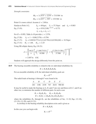
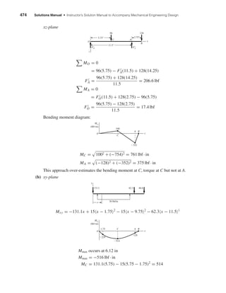
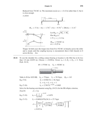
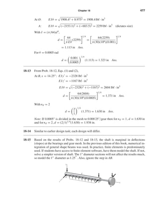
478. 478 Solutions Manual • Instructor’s Solution Manual to Accompany Mechanical Engineering Design
The deflection equations developed in Prob. 18-12 still apply to section OCA.
O: E Iθ = 1908.4 lbf · in3
A: E Iθ = 2259 lbf · in3
(still dictates)
θ =
2259
30(106)(π/64)(1.254)
= 0.000 628 rad
n =
0.001
0.000 628
= 1.59
At gear mesh, B
xy plane
From Prob. 18-12, with I = I1 in section OCA,
yA = −2153.1/E I1
Since yB/A is a cantilever, from Table A-9-1, with I = I2 in section AB
yB/A =
Fx(x − 2l)
2E I2
=
46.6
2E I2
(2.75)[2.75 − 2(2.75)] = −176.2/E I2
∴ yB = yA + yB/A = −
2153.1
30(106)(π/64)(1.254)
−
176.2
30(106)(π/64)(0.8754)
= −0.000 803 rad (magnitude greater than 0.0005 rad)
xz plane
zA = −
683.5
E I1
, zB/A = −
128(2.752
)
2E I2
= −
484
E I2
zB = −
683.5
30(106)(π/64)(1.254)
−
484
30(106)(π/64)(0.8754)
= −0.000 751 rad
θB = (−0.000 803)2 + (0.000 751)2 = 0.001 10 rad
Crowned teeth must be used.
Finite element results: Error in simplified model
θO = 5.47(10−4
) rad 3.0%
θA = 7.09(10−4
) rad 11.4%
θB = 1.10(10−3
) rad 0.0%
z
A
B
x
128 lbf
C
O
x
y
A
B
C
O
46.6 lbf
shi20396_ch18.qxd 8/28/03 4:17 PM Page 478

479. Chapter 18 479
The simplified model yielded reasonable results.
Strength Sut = 72 kpsi, Sy = 39.5 kpsi
At the shoulder at A, x = 10.75 in. From Prob. 18-10,
Mxy = −209.3 lbf · in, Mxz = −293.0 lbf · in, T = 192 lbf · in
M = (−209.3)2 + (−293)2 = 360.0 lbf · in
Se = 0.504(72) = 36.29 kpsi
ka = 2.70(72)−0.265
= 0.869
kb =
1
0.3
−0.107
= 0.879
kc = kd = ke = kf = 1
Se = 0.869(0.879)(36.29) = 27.7 kpsi
From Fig. A-15-8 with D/d = 1.25 and r/d = 0.03, Kts = 1.8.
From Fig. A-15-9 with D/d = 1.25 and r/d = 0.03, Kt = 2.3
From Fig. 7-20 with r = 0.03 in, q = 0.65.
From Fig. 7-21 with r = 0.03 in, qs = 0.83
Eq. (7-31): Kf = 1 + 0.65(2.3 − 1) = 1.85
Kf s = 1 + 0.83(1.8 − 1) = 1.66
Using DE-elliptic,
r =
2Kf Ma
√
3Kf sTm
=
2(1.85)(360)
√
3(1.66)(192)
= 2.413
Sa =
2Sy S2
e
S2
e + S2
y
=
2(39.5)(27.72
)
(27.72) + (39.52)
= 26.0 kpsi
Sm = Sy − Sa = 39.5 − 26.0 = 13.5 kpsi
rcrit =
Sa
Sm
=
26
13.5
= 1.926
r > rcrit
Therefore, the threat is fatigue.
Eq. (18-22),
1
n
=
16
π(13)
4
1.85(360)
27 700
2
+ 3
1.66(192)
39 500
2 1/2
n = 3.92
Perform a similar analysis at the profile keyway under the gear.
The main problem with the design is the undersized shaft overhang with excessive slope
at the gear. The use of crowned-teeth in the gears will eliminate this problem.
shi20396_ch18.qxd 8/28/03 4:17 PM Page 479

480. 480 Solutions Manual • Instructor’s Solution Manual to Accompany Mechanical Engineering Design
18-16 Treat car, truck frame, and wheels as a free body:
Tipping moment = 17 100(72) = 1.231(106
) lbf · in
Force of resisting couple, Fc = 1.231(106
)/59.5 = 20 690 lbf
Force supporting weight, Fw = 42 750/2 = 21 375 lbf
Fr = 17 100 lbf
R1 = Fw + Fc = 21 375 + 20 690 = 42 065 lbf
R2 = Fw − Fc = 21 375 − 20 690 = 685 lbf
For the car and truck as a free body:
Tipping moment = 17 100(72 − 16.5) = 949 050 lbf · in
Gc =
949 050
80
= 11 863 lbf
The force at the journal is Gw = 42 750/2 = 21 375 lbf
Gr = 17 100 lbf
R1 = 21 375 + 11 863 = 33 238 lbf
R2 = 21 375 − 11 863 = 9512 lbf
Wheels and axle as a free body
Axle as a free body:
Couple due to flange force = (17 100)(33/2) = 282 150 lbf · in
Midspan moment:
M = 33 238(40) + 282 150 − 42 065(59.5/2) = 360 240 lbf · in
Since the curvature and wind loads can be from opposite directions, the axle must resist
622 840 lbf · in at either wheel seat and resist 360 240 lbf · in in the center. The bearing
load could be 33 238 lbf at the other bearing. The tapered axle is a consequence of this.
Brake forces are neglected because they are small and induce a moment on the perpen-
dicular plane.
340 690
M
(lbf•in)
622 840
97 498
17 100
17 100
33 238
42 065 685
9512
282 150 lbf•in
17 100
17 100
33͞2
33 238
42 065 685
9512
Gw
Gr
Gw
Gc Gc
72 Ϫ 16.5
42 750
17 100
Fw
Fr
Fw
Fc Fc
72"
42 750
17 100
shi20396_ch18.qxd 8/28/03 4:17 PM Page 480

481. Chapter 18 481
18-17 Some information is brought forward from the solution of Prob. 18-16. At the wheel seat
σ =
32M
πd3
=
32(622 840)
π(73)
= 18 496 psi
At mid-axle
σ =
32(360 240)
π(5.375)3
= 23 630 psi
The stress at the wheel seat consists of the bending stress plus the shrink fit compression
combining for a higher von Mises stress.
18-18 This problem has to be done by successive trials, since Se is a function of shaft size in
Eq. (18-21). The material is SAE 2340 for which Sut = 1226 MPa, Sy = 1130 MPa, and
HB ≥ 368.
Eq. (7-18): ka = 4.51(1226)−0.265
= 0.685
Trial #1: Choose dr = 22 mm
kb =
22
7.62
−0.107
= 0.893
Se = 0.685(0.893)(0.504)(1226) = 378 MPa
dr = d − 2r = 0.75D − 2D/20 = 0.65D
D =
dr
0.65
=
22
0.65
= 33.8 mm
r =
D
20
=
33.8
20
= 1.69 mm
Fig. A-15-14:
d = dr + 2r = 22 + 2(1.69) = 25.4 mm
d
dr
=
25.4
22
= 1.15
r
dr
=
1.69
22
= 0.077
Kt = 1.9
Fig. A-15-15: Kts = 1.5
Fig. 7-20: r = 1.69 mm, q = 0.90
Fig. 7-21: r = 1.69 mm, qs = 0.97
Eq. (7-31): Kf = 1 + 0.90(1.9 − 1) = 1.81
Kf s = 1 + 0.97(1.5 − 1) = 1.49
shi20396_ch18.qxd 8/28/03 4:17 PM Page 481

482. 482 Solutions Manual • Instructor’s Solution Manual to Accompany Mechanical Engineering Design
Eq. (18-21) with d as dr ,
dr =



16(2.5)
π
4
1.81(70)(103
)
378
2
+ 3
1.49(45)(103
)
1130
2 1/2



1/3
= 20.5 mm
Trial #2: Choose dr = 20.5 mm
kb =
20.5
7.62
−0.107
= 0.900
Se = 0.685(0.900)(0.504)(1226) = 381 MPa
D =
dr
0.65
=
20.5
0.65
= 31.5 mm
r =
D
20
=
31.5
20
= 1.58 mm
Figs. A-15-14 and A-15-15:
d = dr + 2r = 20.5 + 2(1.58) = 23.7 mm
d
dr
=
23.7
20.5
= 1.16
r
dr
=
1.58
20.5
= 0.077
We are at the limit of readability of the figures so
Kt = 1.9, Kts = 1.5 q = 0.9, qs = 0.97
∴ Kf = 1.81 Kf s = 1.49
Using Eq. (18-21) produces no changes. Therefore we are done.
Decisions:
dr = 20.5
D =
20.5
0.65
= 31.5 mm, d = 0.75(31.5) = 23.6 mm
Use D = 32 mm, d = 24 mm, r = 1.6 mm Ans.
18-19 Refer to Prob. 18-18. Trial #1, nd = 2.5, dr = 22 mm, Se = 378 MPa, Kf = 1.81,
Kf s = 1.49
Eq. (18-30)
dr =



32(2.5)
π
1.81
70(103
)
(378)
2
+ 1.49
45(103
)
(1130)
2 1/2



1/3
= 20.5 mm
shi20396_ch18.qxd 8/28/03 4:17 PM Page 482

483. Chapter 18 483
Referring to Trial #2 of Prob. 18-18, dr = 20.5 mm and Se = 381 MPa. Substitution into
Eq. (18-30) yields dr = 20.5 mm again. Solution is the same as Prob. 18-18; therefore use
D = 32 mm, d = 24 mm, r = 1.6 mm Ans.
18-20 F cos 20°(d/2) = T, F = 2T/(d cos 20°) = 2(3000)/(6 cos 20°) = 1064 lbf
MC = 1064(4) = 4257 lbf · in
(a) Static analysis using fatigue stress concentration factors and Eq. (6-45):
d =
16n
πSy
4(Kf M)2
+ 3(Kf sT)2 1/2
1/3
=
16(2.5)
π(60 000)
4(1.8)(4257)2
+ 3(1.3)(3000)2 1/2
1/3
= 1.526 in Ans.
(b) ka = 2.70(80)−0.265
= 0.845
Assume d = 2.00 in
kb =
2
0.3
−0.107
= 0.816
Se = 0.845(0.816)(0.504)(80) = 27.8 kpsi
(1) DE-Gerber, Eq. (18-16):
d =



16(2.5)(1.8)(4257)
π(27 800)

1 + 1 + 3
1.3(3000)(27 800)
1.8(4257)(80 000)
2 1/2





1/3
= 1.929 in
Revising kb results in d = 1.927 in Ans.
(2) DE-elliptic using d = 2 in for Se with Eq. (18-21),
d =



16(2.5)
π
4
1.8(4257)
27 800
2
+ 3
1.3(3000)
60 000
2 1/2



1/3
= 1.927 in
Revising kb results in d = 1.926 in Ans.
(3) Soderberg, Eq. (18-30):
d =



32(2.5)
π
1.8
4257
27 800
2
+ 1.3
3000
60 000
2 1/2



1/3
= 1.932 in
Revising kb results in d = 1.930 in Ans.
(4) DE-Goodman, Eq. (18-34):
d =
16(2.5)
π
2
1.8(4257)
27 800
+
√
3
1.3(3000)
80 000
1/3
= 2.008 in Ans.
shi20396_ch18.qxd 8/28/03 4:17 PM Page 483

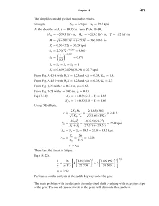
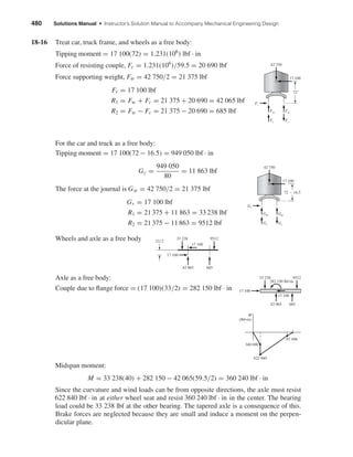
484. 484 Solutions Manual • Instructor’s Solution Manual to Accompany Mechanical Engineering Design
18-21 (a) DE-Gerber, Eqs. (18-13) and (18-15):
A = 4[2.2(600)]2
+ 3[1.8(400)]2 1/2
= 2920 lbf · in
B = 4[2.2(500)]2
+ 3[1.8(300)]2 1/2
= 2391 lbf · in
d =



8(2)(2920)
π(30 000)

1 + 1 +
2(2391)(30 000)
2920(100 000)
2 1/2





1/3
= 1.016 in Ans.
(b) DE-elliptic, Equation prior to Eq. (18-19):
d =
16n
π
A2
S2
e
+
B2
S2
y
1/3
=

16(2)
π
2920
30 000
2
+
2391
80 000
2


1/3
= 1.012 in Ans.
(c) MSS-Soderberg, Eq. (18-28):
d =



32(2)
π
2.22 500
80 000
+
600
30 000
2
+ 1.82 300
80 000
+
400
30 000
2 1/2



1/3
= 1.101 in Ans.
(d) DE-Goodman: Eq. (18-32) can be shown to be
d =
16n
π
A
Se
+
B
Sut
1/3
=
16(2)
π
2920
30 000
+
2391
100 000
1/3
= 1.073 in
Criterion d(in) Compared to DE-Gerber
DE-Gerber 1.016
DE-elliptic 1.012 0.4% lower less conservative
MSS-Soderberg 1.101 8.4% higher more conservative
DE-Goodman 1.073 5.6% higher more conservative
18-22 We must not let the basis of the stress concentration factor, as presented, impose a
viewpoint on the designer. Table A-16 shows Kts as a decreasing monotonic as a function
of a/D. All is not what it seems.
Let us change the basis for data presentation to the full section rather than the net
section.
τ = Ktsτ0 = Ktsτ0
Kts =
32T
π AD3
= Kts
32T
π D3
shi20396_ch18.qxd 8/28/03 4:17 PM Page 484

485. Chapter 18 485
Therefore
Kts =
Kts
A
Form a table:
(a/D) A Kts Kts
0.050 0.95 1.77 1.86
0.075 0.93 1.71 1.84
0.100 0.92 1.68 1.83 ← minimum
0.125 0.89 1.64 1.84
0.150 0.87 1.62 1.86
0.175 0.85 1.60 1.88
0.200 0.83 1.58 1.90
Kts has the following attributes:
• It exhibits a minimum;
• It changes little over a wide range;
• Its minimum is a stationary point minimum at a/D
.
= 0.100;
• Our knowledge of the minima location is
0.075 ≤ (a/D) ≤ 0.125
We can form a design rule: in torsion, the pin diameter should be about 1/10 of the shaft
diameter, for greatest shaft capacity. However, it is not catastrophic if one forgets the rule.
18-23 Preliminaries:
T =
63 025(4.5)
112
= 2532 lbf · in
Wt
=
T
r
=
2532
8/2
= 633 lbf
W =
633
cos 20°
= 674 lbf
R1 = 674
3
10
= 202 lbf
R2 = 674
7
10
= 472 lbf
Mmax = 202(7) = 1414 lbf · in
R1 R2
674 lbf
7" 3"
10"
shi20396_ch18.qxd 8/28/03 4:17 PM Page 485

486. 486 Solutions Manual • Instructor’s Solution Manual to Accompany Mechanical Engineering Design
Is the task strength-controlled or distortion-controlled? With regards to distortion use
n = 2 in Eq. (18-1):
dL =
32(2)(674)(3)(32
− 102
)
3π(30)(106)(10)(0.001)
1/4
= 1.43 in
Eq. (18-2):
dR =
32(2)(674)(7)(102
− 72
)
3π(30)(106)(10)(0.001)
1/4
= 1.53 in
For the gearset, use θAB developed in Prob. 18-4 solution. To the left of the load,
θAB =
Fb
6E Il
(3x2
+ b2
− l2
)
Incorporating I = πd4
/64 and nd,
d =
32nd Fb
3π Elθall
(3x2
+ b2
− l2
)
1/4
At the gearset, x = 7 with θall = 0.000 25 (apportioning gearmesh slope equally).
d ≤
32(2)(674)(3)[3(72
) + 32
− 102
]
3π(30)(106)(10)(0.000 25)
1/4
≤ 1.789 in
Since 1.789 > 1.75 in, angular deflection of the matching gear should be less than
0.000 25 rad. Crowned gears should thus be used, or nd scutinized for reduction.
Concerning strength: For Kf
.
= 2, Kf s
.
= 1.5, Se
.
= Sut/4, Sy
.
= Sut/2 in Eq. (18-1):
d3
=
16n
π
4
2(1414)
Sut/4
2
+ 3
1.5(2532)
Sut/2
2 1/2
Solving for Sut and using n = 2 and d = 1.75 in
Sut =
16(2)
π(1.753)
{4[4(2)(1414)]2
+ 3[2(1.5)(2532)]2
}1/2
= 49 740 psi
This gives an approximate idea of the shaft material strength necessary and helps identify
an initial material.
With this perspective students can begin.
18-24 This task is a change of pace. Let s be the scale factor of the model, and subscript m
denote ‘model.’
lm = sl
σ =
Mc
I
, σm = σ
Mm =
σm Im
cm
=
σs4
I
sc
= s3
M Ans.
shi20396_ch18.qxd 8/28/03 4:17 PM Page 486

487. Chapter 18 487
The load that causes bending is related to reaction and distance.
Mm = Rmam =
Fmbmam
lm
Solving for Fm gives
Fm =
Mmlm
ambm
=
s3
M(sl)
(sa)(sb)
= s2
F Ans.
For deflection use Table A-9-6 for section AB,
ym =
Fmbmxm
6Em Imlm
x2
m + b2
m − l2
m
=
(s2
F)(sb)(sx)
6E(s4 I)(sl)
(s2
x2
+ s2
b2
− s2
l2
)
= sy Ans. (as expected)
For section BC, the same is expected.
For slope, consider section AB
yAB = θAB =
Fb
6E Il
(3x2
+ b2
− l2
)
θm =
s2
F(sb)
6E(s4 I)(sl)
(3s2
x2
+ s2
b2
− s2
l2
) = θ
The same will apply to section BC
Summary:
Slope: ym = y
Deflection: ym = sy =
y
2
Moment: Mm = s3
M =
M
8
Force: Fm = s2
F =
F
4
These relations are applicable for identical materials and stress levels.
18-25 If you have a finite element program available, it is highly recommended. Beam deflec-
tion programs can be implemented but this is time consuming and the programs have
narrow applications. Here we will demonstrate how the problem can be simplified and
solved using singularity functions.
Deflection: First we will ignore the steps near the bearings where the bending moments
are low. Thus let the 30 mm dia. be 35 mm. Secondly, the 55 mm dia. is very thin, 10 mm.
The full bending stresses will not develop at the outer fibers so full stiffness will not
develop either. Thus, ignore this step and let the diameter be 45 mm.
shi20396_ch18.qxd 8/28/03 4:17 PM Page 487

488. 488 Solutions Manual • Instructor’s Solution Manual to Accompany Mechanical Engineering Design
Statics: Left support: R1 = 7(315 − 140)/315 = 3.889 kN
Right support: R2 = 7(140)/315 = 3.111 kN
Determine the bending moment at each step.
x(mm) 0 40 100 140 210 275 315
M(N · m) 0 155.56 388.89 544.44 326.67 124.44 0
I35 = (π/64)(0.0354
) = 7.366(10−8
) m4
, I40 = 1.257(10−7
) m4
, I45 = 2.013(10−7
) m4
Plot M/I as a function of x.
x(m) M/I (109
N/m3
) Step Slope Slope
0 0 52.8
0.04 2.112
0.04 1.2375 −0.8745 30.942 −21.86
0.1 3.094
0.1 1.932 −1.162 19.325 −11.617
0.14 2.705
0.14 2.705 0 −15.457 −34.78
0.21 1.623
0.21 2.6 0.977 −24.769 −9.312
0.275 0.99
0.275 1.6894 0.6994 −42.235 −17.47
0.315 0
The steps and the change of slopes are evaluated in the table. From these, the function
M/I can be generated:
M/I = 52.8x − 0.8745 x − 0.04 0
− 21.86 x − 0.04 1
− 1.162 x − 0.1 0
− 11.617 x − 0.1 1
− 34.78 x − 0.14 1
+ 0.977 x − 0.21 0
− 9.312 x − 0.21 1
+ 0.6994 x − 0.275 0
− 17.47 x − 0.275 1
109
Integrate twice:
E
dy
dx
= 26.4x2
− 0.8745 x − 0.04 1
− 10.93 x − 0.04 2
− 1.162 x − 0.1 1
− 5.81 x − 0.1 2
− 17.39 x − 0.14 2
+ 0.977 x − 0.21 1
− 4.655 x − 0.21 2
+ 0.6994 x − 0.275 1
− 8.735 x − 0.275 2
+ C1 109
(1)
Ey = 8.8x3
− 0.4373 x − 0.04 2
− 3.643 x − 0.04 3
− 0.581 x − 0.1 2
− 1.937 x − 0.1 3
− 5.797 x − 0.14 3
+ 0.4885 x − 0.21 2
− 1.552 x − 0.21 3
+ 0.3497 x − 0.275 2
− 2.912 x − 0.275 3
+ C1x + C2 109
4
0
1
2
3
0 0.350.30.250.20.15
x (mm)
M͞I(109
N͞m3
)
0.10.05
shi20396_ch18.qxd 8/28/03 4:17 PM Page 488

489. Chapter 18 489
Boundary conditions: y = 0 at x = 0 yields C2 = 0;
y = 0 at x = 0.315m yields C1 = −0.295 25 N/m2
.
Equation (1) with C1 = −0.295 25 provides the slopes at the bearings and gear. The
following table gives the results in the second column. The third column gives the results
from a similar finite element model. The fourth column gives the result of a full model
which models the 35 and 55 mm diameter steps.
x (mm) θ (rad) F.E. Model Full F.E. Model
0 −0.0014260 −0.0014270 −0.0014160
140 −0.0001466 −0.0001467 −0.0001646
315 0.0013120 0.0013280 0.0013150
The main discrepancy between the results is at the gear location (x = 140 mm). The
larger value in the full model is caused by the stiffer 55 mm diameter step. As was stated
earlier, this step is not as stiff as modeling implicates, so the exact answer is somewhere
between the full model and the simplified model which in any event is a small value. As
expected, modeling the 30 mm dia. as 35 mm does not affect the results much.
It can be seen that the allowable slopes at the bearings are exceeded. Thus, either the
load has to be reduced or the shaft “beefed” up. If the allowable slope is 0.001 rad, then
the maximum load should be Fmax = (0.001/0.001 46)7 = 4.79 kN. With a design factor
this would be reduced further.
To increase the stiffness of the shaft, increase the diameters by (0.001 46/0.001)1/4
=
1.097. Form a table:
Old d, mm 20.00 30.00 35.00 40.00 45.00 55.00
New ideal d, mm 21.95 32.92 38.41 43.89 49.38 60.35
Rounded up d, mm 22.00 34.00 40.00 44.00 50.00 62.00
Repeating the full finite element model results in
x = 0: θ = −9.30 × 10−4
rad
x = 140 mm: θ = −1.09 × 10−4
rad
x = 315 mm: θ = 8.65 × 10−4
rad
Well within our goal. Have the students try a goal of 0.0005 rad at the bearings.
Strength: Due to stress concentrations and reduced shaft diameters, there are a number of
locations to look at. A table of nominal stresses is given below. Note that torsion is only
to the right of the 7 kN load. Using σ = 32M/(πd3
) and τ = 16T/(πd3
),
x (mm) 0 15 40 100 110 140 210 275 300 330
σ (MPa) 0 22.0 37.0 61.9 47.8 60.9 52.0 39.6 17.6 0
τ (MPa) 0 0 0 0 0 6 8.5 12.7 20.2 68.1
σ (MPa) 0 22.0 37.0 61.9 47.8 61.8 53.1 45.3 39.2 118.0
Table A-20 for AISI 1020 CD steel: Sut = 470 MPa, Sy = 390 MPa
shi20396_ch18.qxd 8/28/03 4:17 PM Page 489

490. 490 Solutions Manual • Instructor’s Solution Manual to Accompany Mechanical Engineering Design
At x = 210 mm:
ka = 4.51(470)−0.265
= 0.883, kb = (40/7.62)−0.107
= 0.837
Se = 0.883(0.837)(0.504)(470) = 175 MPa
D/d = 45/40 = 1.125, r/d = 2/40 = 0.05.
From Figs. A-15-8 and A-15-9, Kt = 1.9 and Kts = 1.32.
From Figs. 7-20 and 7-21, q = 0.75 and qs = 0.92,
Kf = 1 + 0.75(1.9 − 1) = 1.68, and Kf s = 1 + 0.92(1.32 − 1) = 1.29.
From Eq. (18-22),
1
n
=
16
π(0.04)3
4
1.68(544.44)
175(106)
2
+ 3
1.29(107)
390(106)
2 1/2
n = 1.20
Depending on the application, this may be too low.
At x = 330 mm: The von Mises stress is the highest but it comes from the steady torque
only.
D/d = 30/20 = 1.5, r/d = 2/20 = 0.1 ⇒ Kts = 1.42,
qs = 0.92 ⇒ Kf s = 1.39
1
n
=
16
π(0.02)3
√
3
1.39(107)
390(106)
n = 2.38
Check the other locations.
If worse-case is at x = 210 mm, the changes discussed for the slope criterion will im-
prove the strength issue.
18-26 In Eq. (18-37) set
I =
πd4
64
, A =
πd2
4
to obtain
ω =
π
l
2
d
4
gE
γ
(1)
or
d =
4l2
ω
π2
γ
gE
(2)
(a) From Eq. (1) and Table A-5,
ω =
π
24
2
1
4
386(30)(106)
0.282
= 868 rad/s Ans.
(b) From Eq. (2),
d =
4(24)2
(2)(868)
π2
0.282
386(30)(106)
= 2 in Ans.
shi20396_ch18.qxd 8/28/03 4:17 PM Page 490

491. Chapter 18 491
(c) From Eq. (2),
lω =
π2
4
d
l
gE
γ
Since d/l is the same regardless of the scale.
lω = constant = 24(868) = 20 832
ω =
20 832
12
= 1736 rad/s Ans.
Thus the first critical speed doubles.
18-27 From Prob. 18-26, ω = 868 rad/s
A = 0.7854 in2
, I = 0.04909 in4
, γ = 0.282 lbf/in3
,
E = 30(106
) psi, w = Aγl = 0.7854(0.282)(24) = 5.316 lbf
One element:
Eq. (18-37) δ11 =
12(12)(242
− 122
− 122
)
6(30)(106)(0.049 09)(24)
= 1.956(10−4
) in/lbf
y1 = w1δ11 = 5.316(1.956)(10−4
) = 1.0398(10−3
) in
y2
1 = 1.0812(10−6
)
wy = 5.316(1.0398)(10−3
) = 5.528(10−3
)
wy2
= 5.316(1.0812)(10−6
) = 5.748(10−6
)
ω1 = g
wy
wy2
= 386
5.528(10−3)
5.748(10−6)
= 609 rad/s (30% low)
Two elements:
δ11 = δ22 =
18(6)(242
− 182
− 62
)
6(30)(106)(0.049 09)(24)
= 1.100(10−4
) in/lbf
δ12 = δ21 =
6(6)(242
− 62
− 62
)
6(30)(106)(0.049 09)(24)
= 8.556(10−5
) in/lbf
y1 = w1δ11 + w2δ12 = 2.658(1.100)(10−4
) + 2.658(8.556)(10−5
)
= 5.198(10−4
) in = y2,
y2
1 = y2
2 = 2.702(10−7
) in2
wy = 2(2.658)(5.198)(10−4
) = 2.763(10−3
)
wy2
= 2(2.658)(2.702)(10−7
) = 1.436(10−6
)
ω1 = 386
2.763(10−3)
1.436(10−6)
= 862 rad/s (0.7% low)
2.658 lbf2.658 lbf
6" 6" 6" 6"
shi20396_ch18.qxd 8/28/03 4:17 PM Page 491

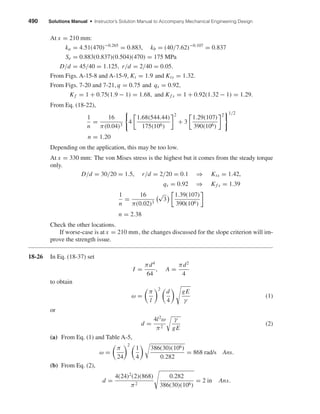
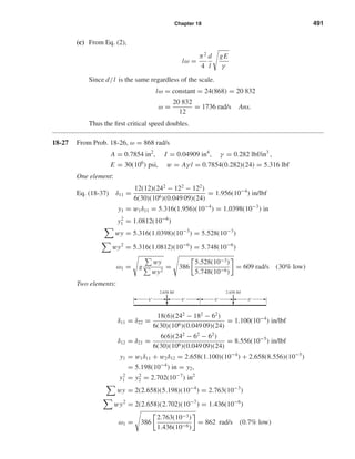
492. 492 Solutions Manual • Instructor’s Solution Manual to Accompany Mechanical Engineering Design
Three elements:
δ11 = δ33 =
20(4)(242
− 202
− 42
)
6(30)(106)(0.049 09)(24)
= 6.036(10−5
) in/lbf
δ22 =
12(12)(242
− 122
− 122
)
6(30)(106)(0.049 09)(24)
= 1.956(10−4
) in/lbf
δ12 = δ32 =
12(4)(242
− 122
− 42
)
6(30)(106)(0.049 09)(24)
= 9.416(10−5
) in/lbf
δ13 =
4(4)(242
− 42
− 42
)
6(30)(106)(0.049 09)(24)
= 4.104(10−5
) in/lbf
y1 = 1.772[6.036(10−5
) + 9.416(10−5
) + 4.104(10−5
)] = 3.465(10−4
) in
y2 = 1.772[9.416(10−5
) + 1.956(10−4
) + 9.416(10−5
)] = 6.803(10−4
) in
y3 = 1.772[4.104(10−5
) + 9.416(10−5
) + 6.036(10−5
)] = 3.465(10−4
) in
wy = 2.433(10−3
), wy2
= 1.246(10−6
)
ω1 = 386
2.433(10−3)
1.246(10−6)
= 868 rad/s (same as in Prob. 18-26)
The point was to show that convergence is rapid using a static deflection beam equation.
The method works because:
• If a deflection curve is chosen which meets the boundary conditions of moment-free
and deflection-free ends, and in this problem, of symmetry, the strain energy is not very
sensitive to the equation used.
• Since the static bending equation is available, and meets the moment-free and deflection-
free ends, it works.
18-28 (a) For two bodies, Eq. (18-39) is
(m1δ11 − 1/ω2
) m2δ12
m1δ21 (m2δ22 − 1/ω2
)
= 0
Expanding the determinant yields,
1
ω2
2
− (m1δ11 + m2δ22)
1
ω2
1
+ m1m2(δ11δ22 − δ12δ21) = 0 (1)
Eq. (1) has two roots 1/ω2
1 and 1/ω2
2 . Thus
1
ω2
−
1
ω2
1
1
ω2
−
1
ω2
2
= 0
1.772 lbf1.772 lbf1.772 lbf
4"4" 8" 8"
shi20396_ch18.qxd 8/28/03 4:17 PM Page 492

493. Chapter 18 493
or,
1
ω2
2
+
1
ω2
1
+
1
ω2
2
1
ω
2
+
1
ω2
1
1
ω2
2
= 0 (2)
Equate the third terms of Eqs. (1) and (2), which must be identical.
1
ω2
1
1
ω2
2
= m1m2(δ11δ22 − δ12δ21) ⇒
1
ω2
2
= ω2
1m1m2(δ11δ22 − δ12δ21)
and it follows that
ω2 =
1
ω1
g2
w1w2(δ11δ22 − δ12δ21)
Ans.
(b) In Ex. 18-5, Part (b) the first critical speed of the two-disk shaft (w1 = 35 lbf,
w2 = 55 lbf) is ω1 = 124.7 rad/s. From part (a), using influence coefficients
ω2 =
1
124.7
3862
35(55)[2.061(3.534) − 2.2342](10−8)
= 466 rad/s Ans.
18-29 In Eq. (18-35) the term I/A appears. For a hollow unform diameter shaft,
I
A
=
π d4
o − d4
i /64
π d2
o − d2
i /4
=
1
16
d2
o + d2
i d2
o − d2
i
d2
o − d2
i
=
1
4
d2
o + d2
i
This means that when a solid shaft is hollowed out, the critical speed increases beyond
that of the solid shaft. By how much?
1
4 d2
o + d2
i
1
4 d2
o
= 1 +
di
do
2
The possible values of di are 0 ≤ di ≤ do , so the range of critical speeds is
ωs
√
1 + 0 to about ωs
√
1 + 1
or from ωs to
√
2ωs . Ans.
18-30 All steps will be modeled using singularity functions with a spreadsheet (see next page).
Programming both loads will enable the user to first set the left load to 1, the right load to
0 and calculate δ11 and δ21. Then setting left load to 0 and the right to 1 to get δ12 and
δ22. The spreadsheet shown on the next page shows the δ11 and δ21 calculation. Table for
M/I vs x is easy to make. The equation for M/I is:
M/I = D13x + C15 x − 1 0
+ E15 x − 1 1
+ E17 x − 2 1
+ C19 x − 9 0
+ E19 x − 9 1
+ E21 x − 14 1
+ C23 x − 15 0
+ E23 x − 15 1
shi20396_ch18.qxd 8/28/03 4:17 PM Page 493

494. 494 Solutions Manual • Instructor’s Solution Manual to Accompany Mechanical Engineering Design
Integrating twice gives the equation for Ey. Boundary conditions y = 0 at x = 0 and at
x = 16 inches provide integration constants (C2 = 0). Substitution back into the deflec-
tion equation at x = 2, 14 inches provides the δ’s. The results are: δ11 − 2.917(10−7
),
δ12 = δ21 = 1.627(10−7
), δ22 = 2.231(10−7
). This can be verified by finite element
analysis.
y1 = 20(2.917)(10−7
) + 35(1.627)(10−7
) = 1.153(10−5
)
y2 = 20(1.627)(10−7
) + 35(2.231)(10−7
) = 1.106(10−5
)
y2
1 = 1.329(10−10
), y2
2 = 1.224(10−10
)
wy = 6.177(10−4
), wy2
= 6.942(10−9
)
Neglecting the shaft, Eq. (18-36) gives
ω1 = 386
6.177(10−4)
6.942(10−9)
= 5860 rad/s or 55 970 rev/min Ans.
A B C D E F G H I
1 F1 = 1 F2 = 0 R1 = 0.875 (left reaction)
2
3 x M I1 = I4 = 0.7854
4 0 0 I2 = 1.833
5 1 0.875 I3 = 2.861
6 2 1.75
7 9 0.875
8 14 0.25
9 15 0.125
10 16 0
11
12 x M/I step slope slope
13 0 0 1.114 082
14 1 1.114 082
15 1 0.477 36 −0.636 722 477 0.477 36 −0.636 72
16 2 0.954 719
17 2 0.954 719 0 −0.068 19 −0.545 55
18 9 0.477 36
19 9 0.305 837 −0.171 522 4 −0.043 69 0.024 503
20 14 0.087 382
21 14 0.087 382 0 −0.043 69 0
22 15 0.043 691
23 15 0.159 155 0.115 463 554 −0.159 15 −0.115 46
24 16 0
25
shi20396_ch18.qxd 8/28/03 4:17 PM Page 494

495. Chapter 18 495
A B C D E F G H I
26 C1 = −4.906 001 093
27
28
29 δ11 = 2.91701E-07
30 δ21 = 1.6266E-07
Repeat for F1 = 0 and F2 = 1.
Modeling the shaft separately using 2 elements gives approximately
The spreadsheet can be easily modified to give
δ11 = 9.605(10−7
), δ12 = δ21 = 5.718(10−7
), δ22 = 5.472(10−7
)
y1 = 1.716(10−5
), y2 = 1.249(10−5
), y2
1 = 2.946(10−10
),
y2
2 = 1.561(10−10
), wy = 3.316(10−4
), wy2
= 5.052(10−9
)
ω1 = 386
3.316(10−4)
5.052(10−9)
= 5034 rad/s Ans.
A finite element model of the exact shaft gives ω1 = 5340 rad/s. The simple model is
5.7% low.
Combination Using Dunkerley’s equation, Eq. (18-45):
1
ω2
1
=
1
58602
+
1
50342
⇒ 3819 rad/s Ans.
18-31 and 18-32 With these design tasks each student will travel different paths and almost all
details will differ. The important points are
• The student gets a blank piece of paper, a statement of function, and some
constraints–explicit and implied.At this point in the course, this is a good experience.
• It is a good preparation for the capstone design course.
R1 R2
11 lbf11.32 lbf
4.5" 3.5"
9"
3.5"4.5"
0.8
1
1.2
0
0.2
0.4
0.6
0 1614121086
x (in)
M(lbf•in)
42
shi20396_ch18.qxd 8/28/03 4:17 PM Page 495

496. • The adequacy of their design must be demonstrated and possibly include a designer’s
notebook.
• Many of the fundaments of the course, based on this text and this course, are useful. The
student will find them useful and notice that he/she is doing it.
• Don’t let the students create a time sink for themselves. Tell them how far you want
them to go.
18-33 I used this task as a final exam when all of the students in the course had consistent
test scores going into the final examination; it was my expectation that they would not
change things much by taking the examination.
This problem is a learning experience. Following the task statement, the following
guidance was added.
• Take the first half hour, resisting the temptation of putting pencil to paper, and decide
what the problem really is.
• Take another twenty minutes to list several possible remedies.
• Pick one, and show your instructor how you would implement it.
The students’ initial reaction is that he/she does not know much from the problem
statement. Then, slowly the realization sets in that they do know some important things
that the designer did not. They knew how it failed, where it failed, and that the design
wasn’t good enough; it was close, though.
Also, a fix at the bearing seat lead-in could transfer the problem to the shoulder fillet,
and the problem may not be solved.
To many students’s credit, they chose to keep the shaft geometry, and selected a new
material to realize about twice the Brinell hardness.
496 Solutions Manual • Instructor’s Solution Manual to Accompany Mechanical Engineering Design
shi20396_ch18.qxd 8/28/03 4:17 PM Page 496