Downloaded 135 times
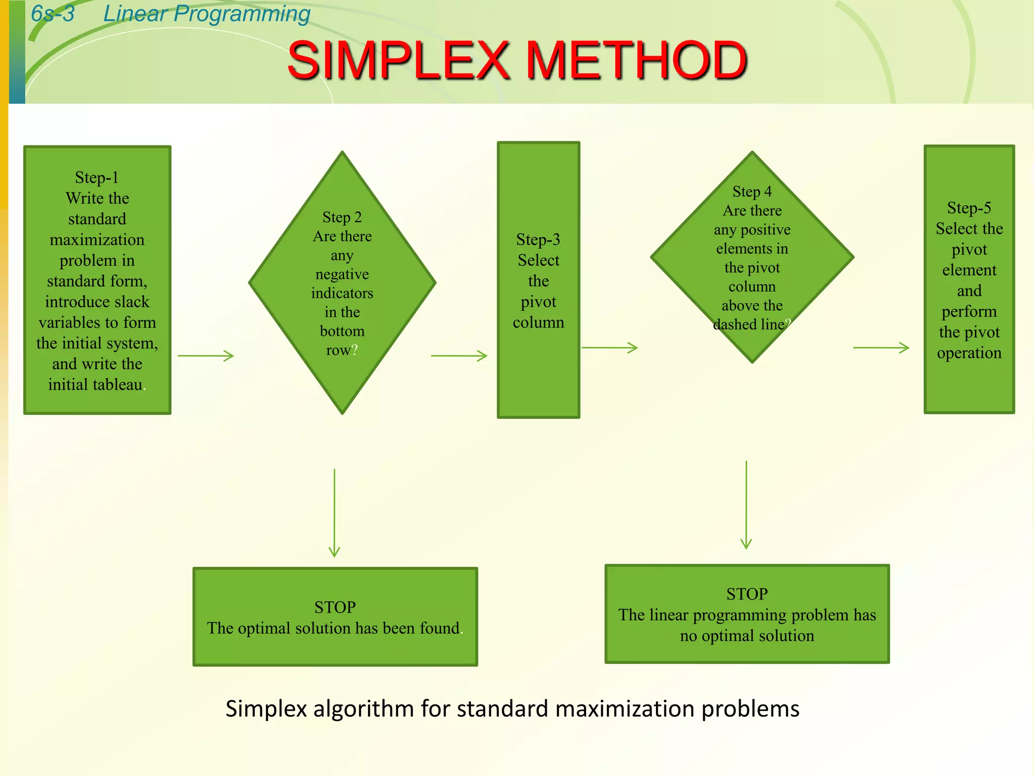
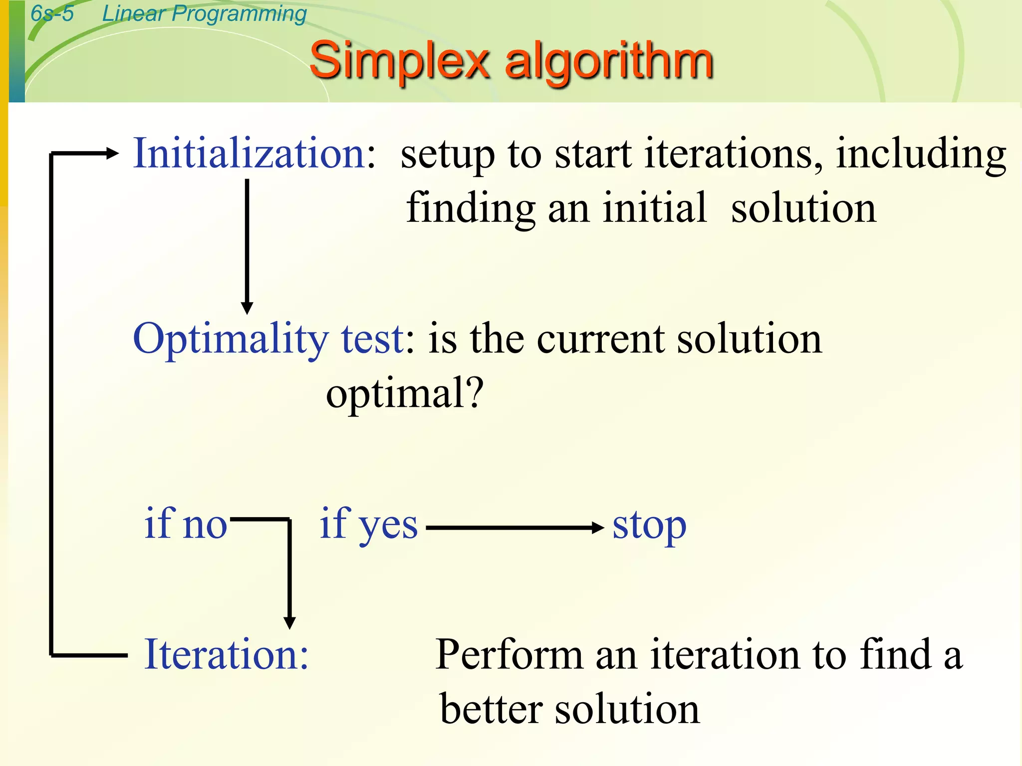
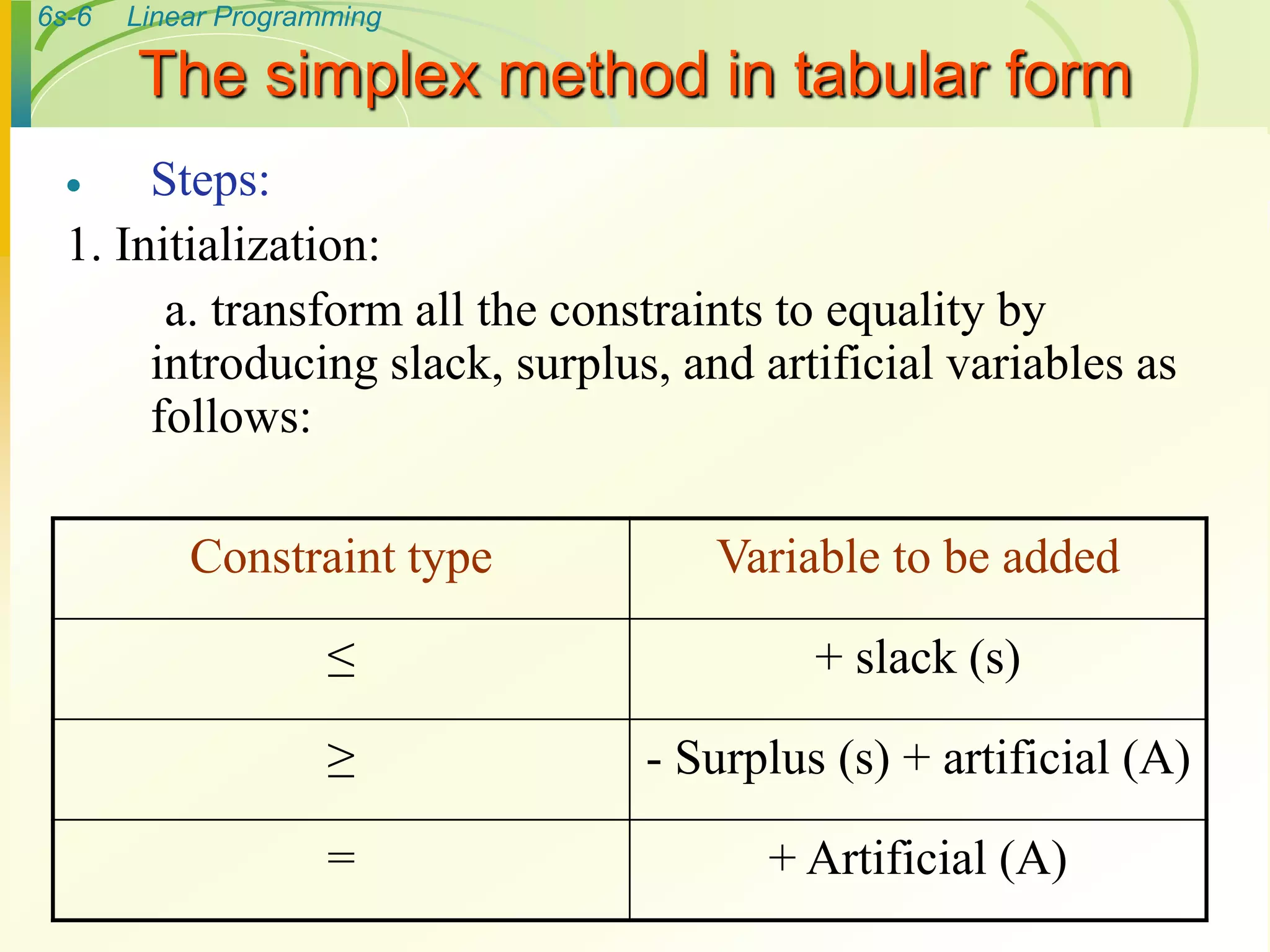
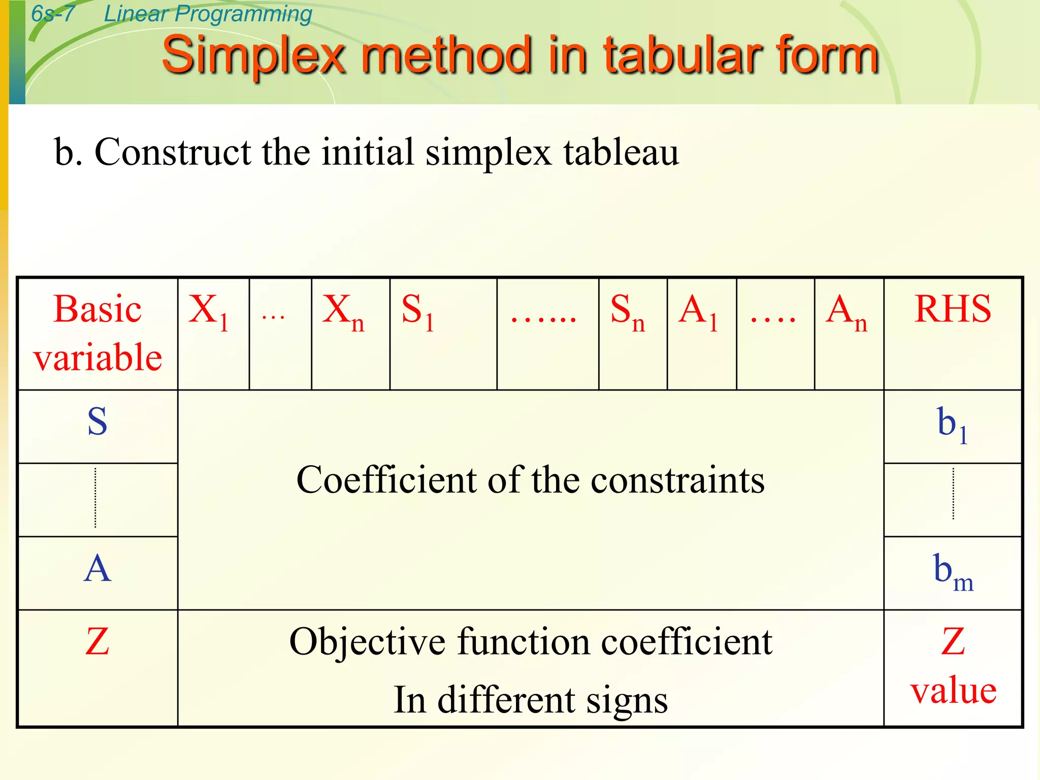
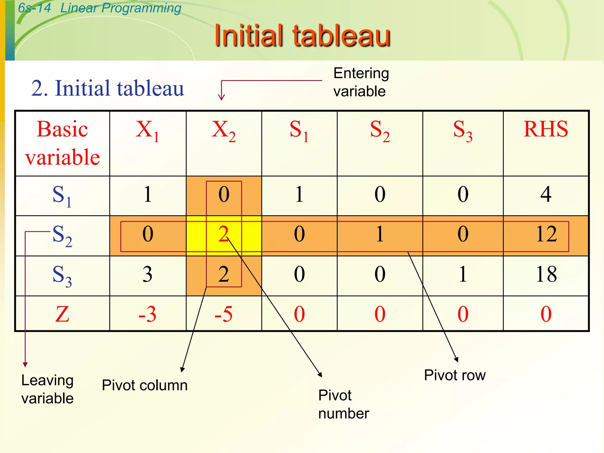
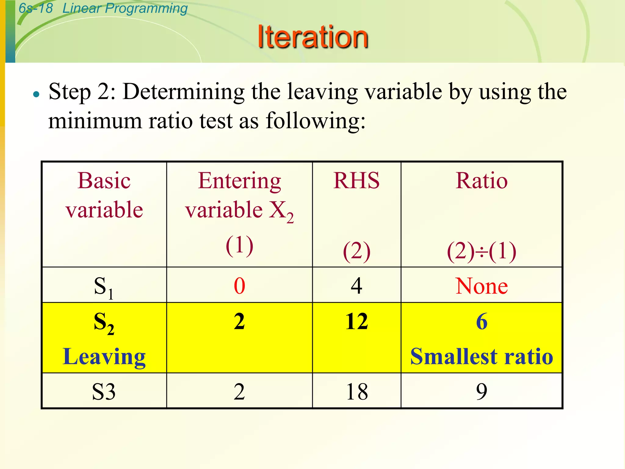
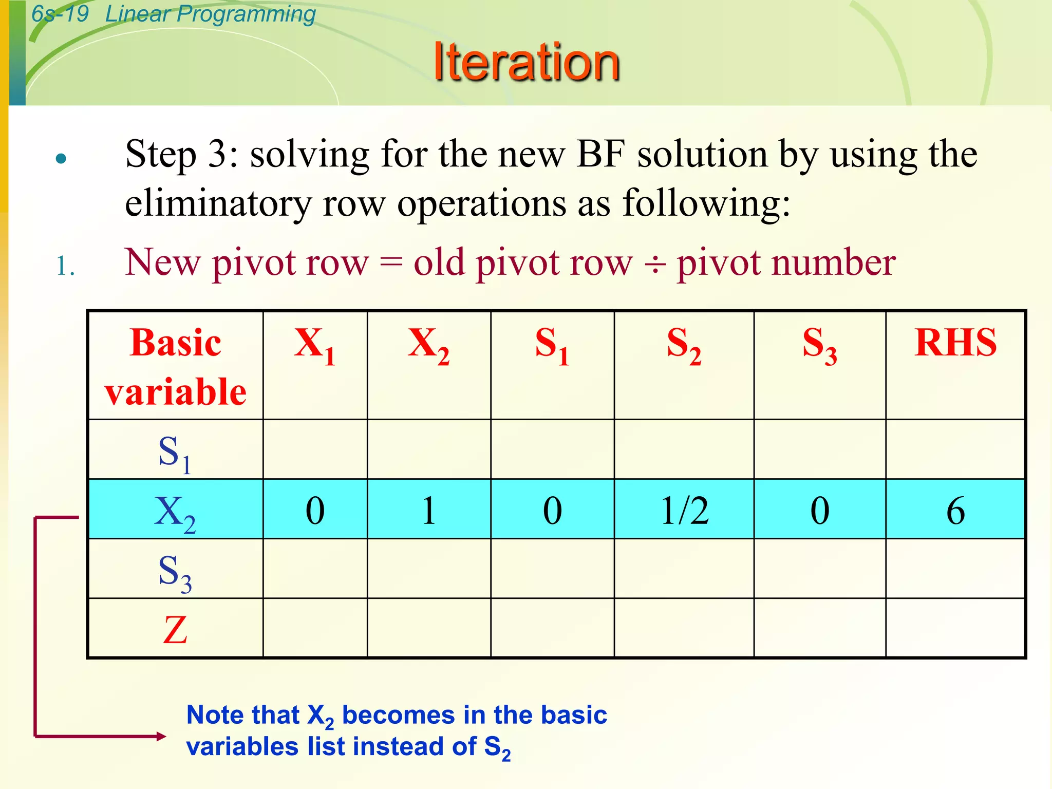
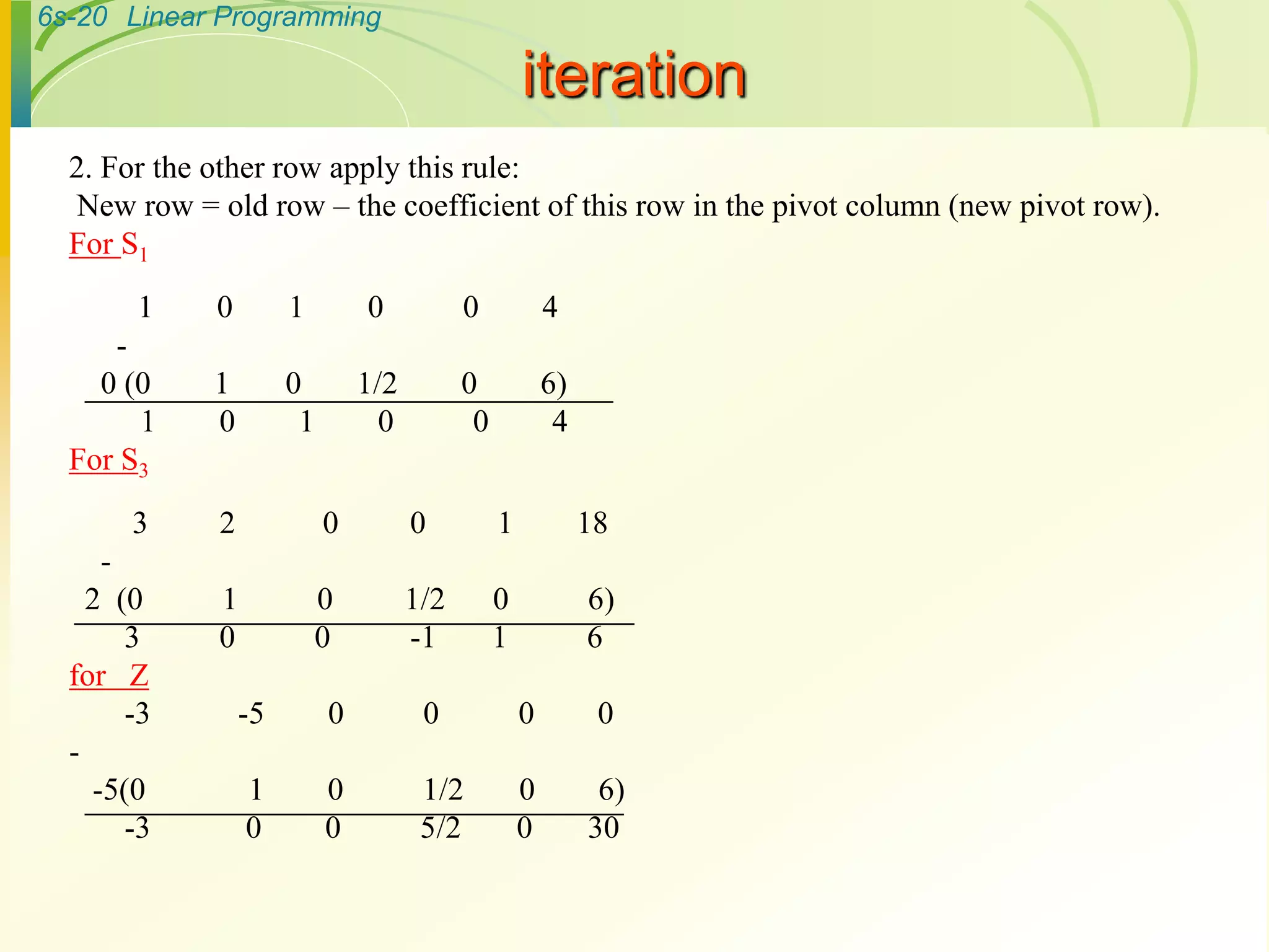
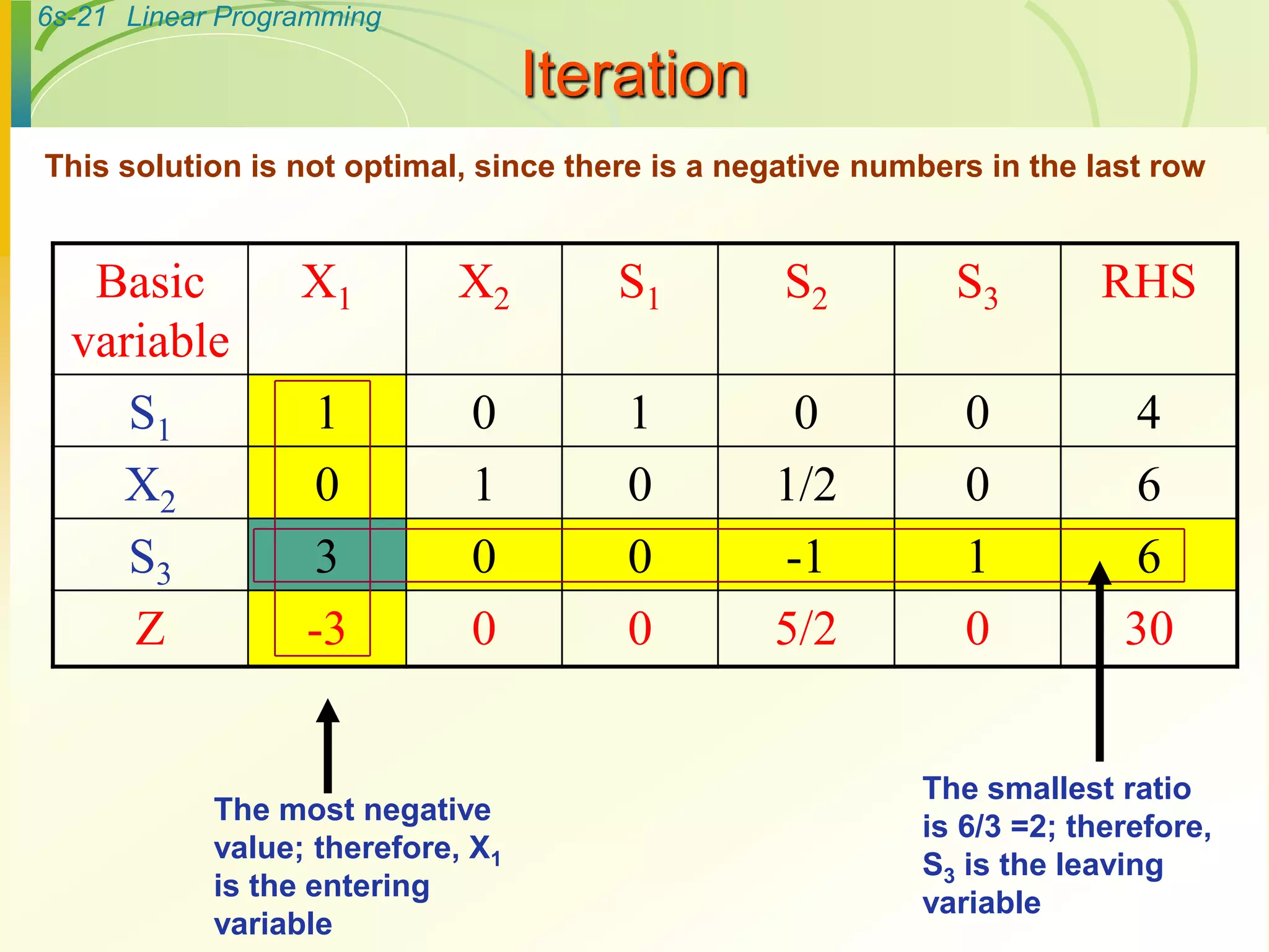
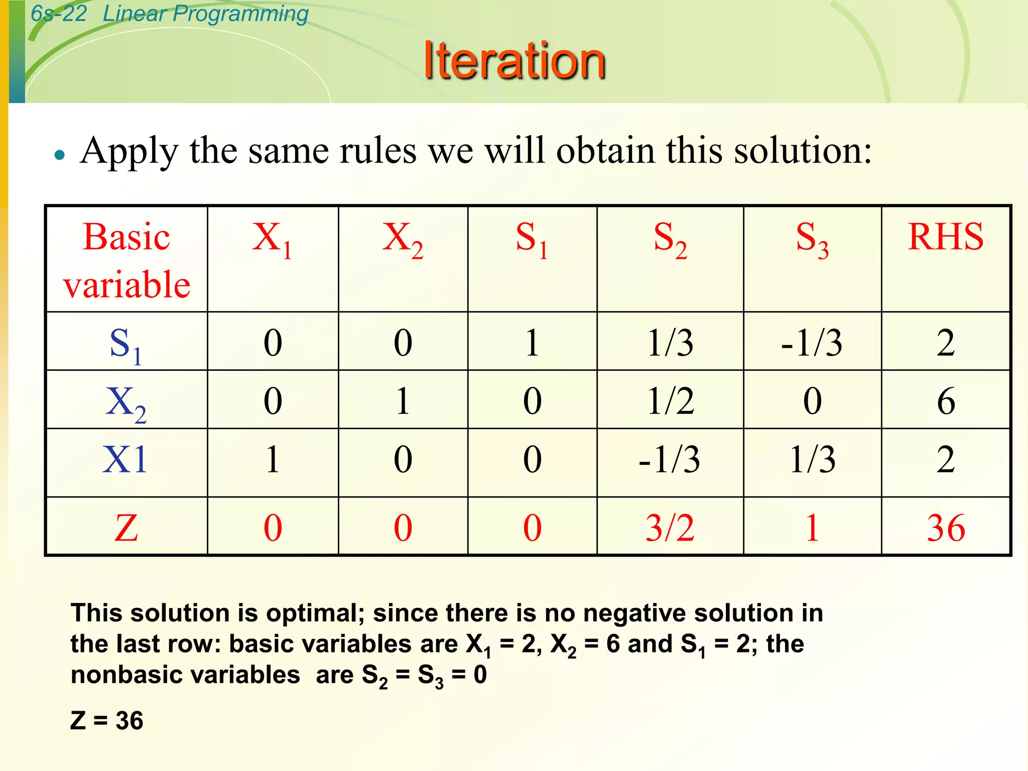
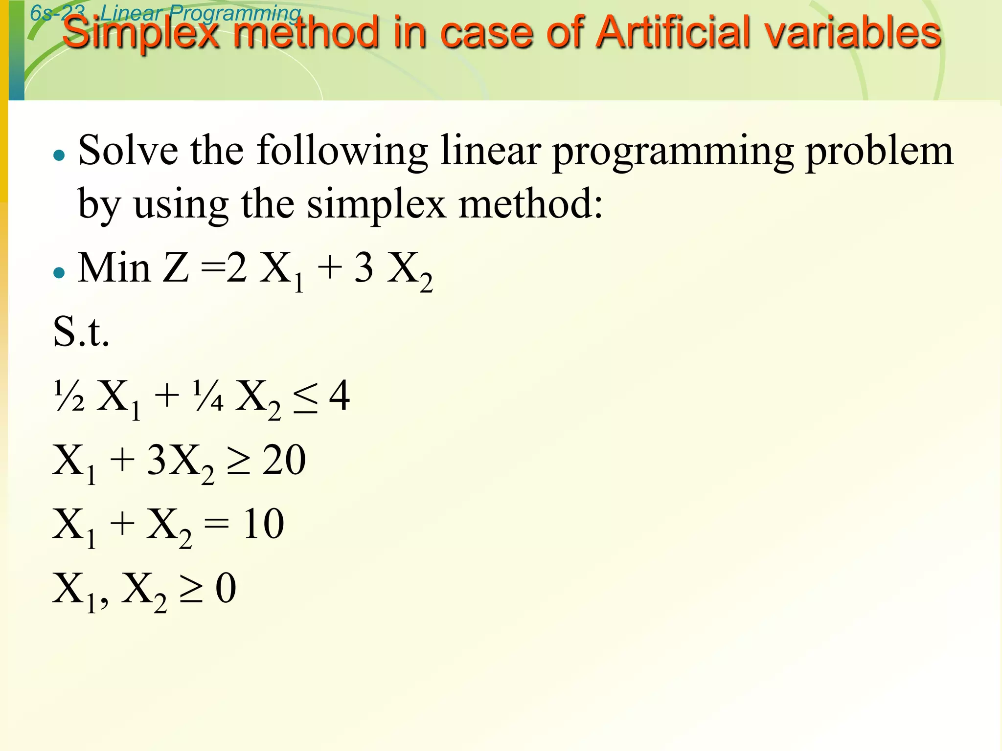
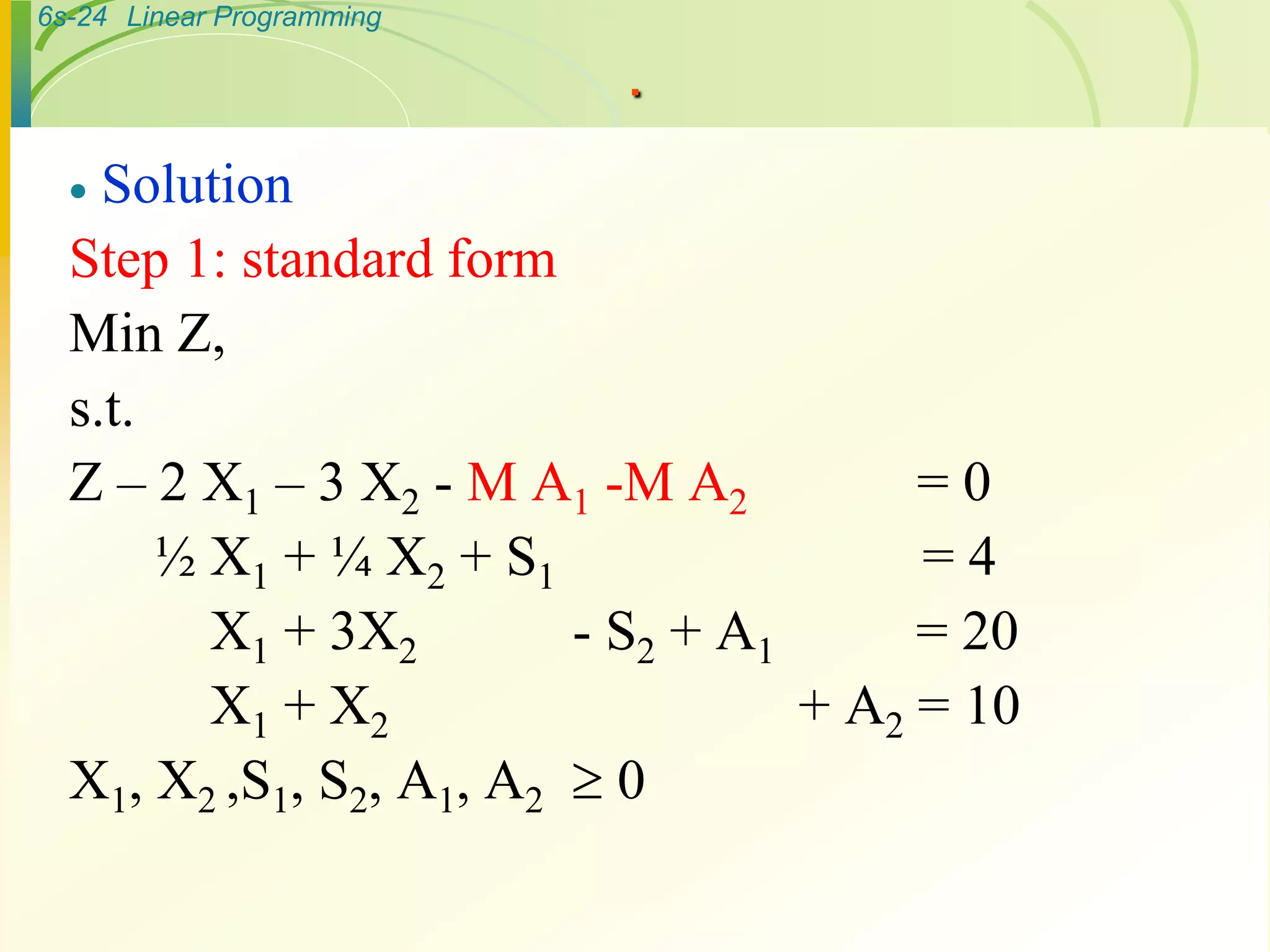
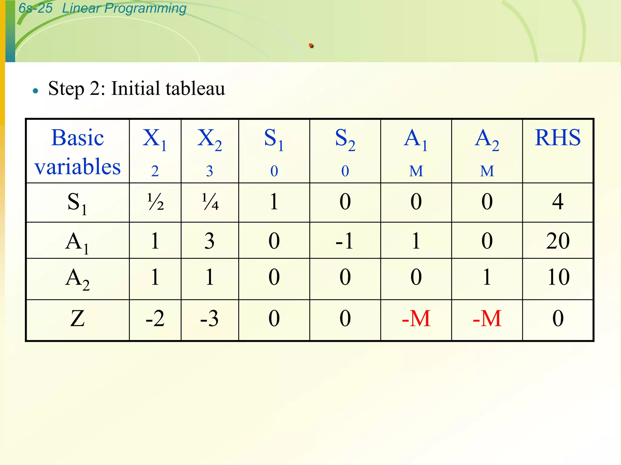
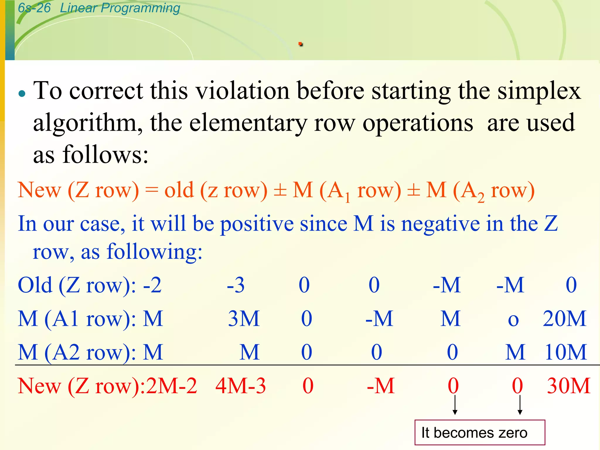
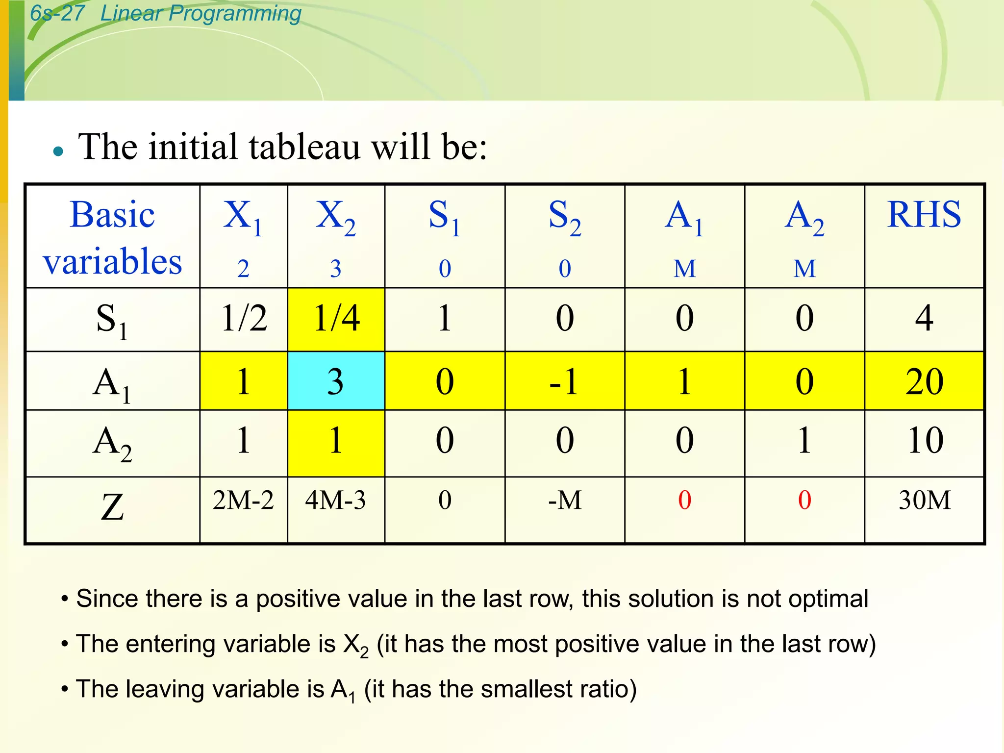
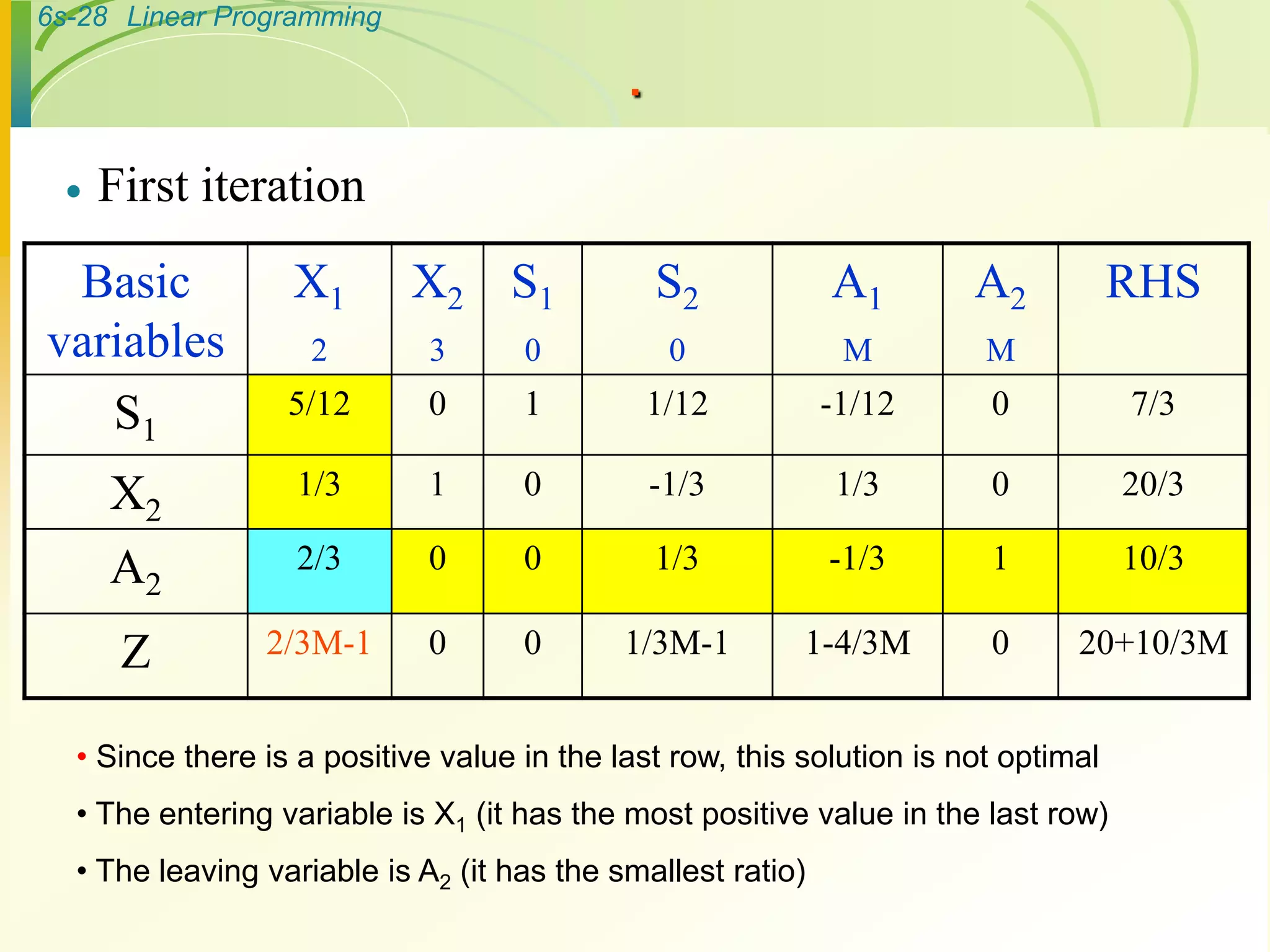
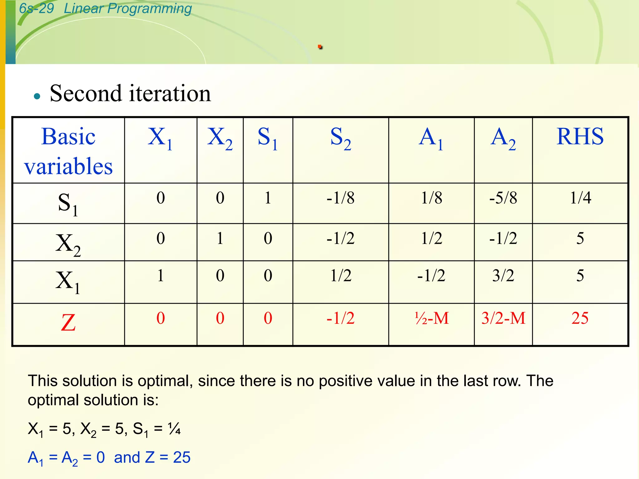

The document provides an overview of the simplex method for solving linear programming problems. It discusses: - The simplex method is an iterative algorithm that generates a series of solutions in tabular form called tableaus to find an optimal solution. - It involves writing the problem in standard form, introducing slack variables, and constructing an initial tableau. - The method then performs iterations involving selecting a pivot column and row, and applying row operations to generate new tableaus until an optimal solution is found. - It also discusses how artificial variables are introduced for problems with non-strict inequalities and provides an example solved using the simplex method.