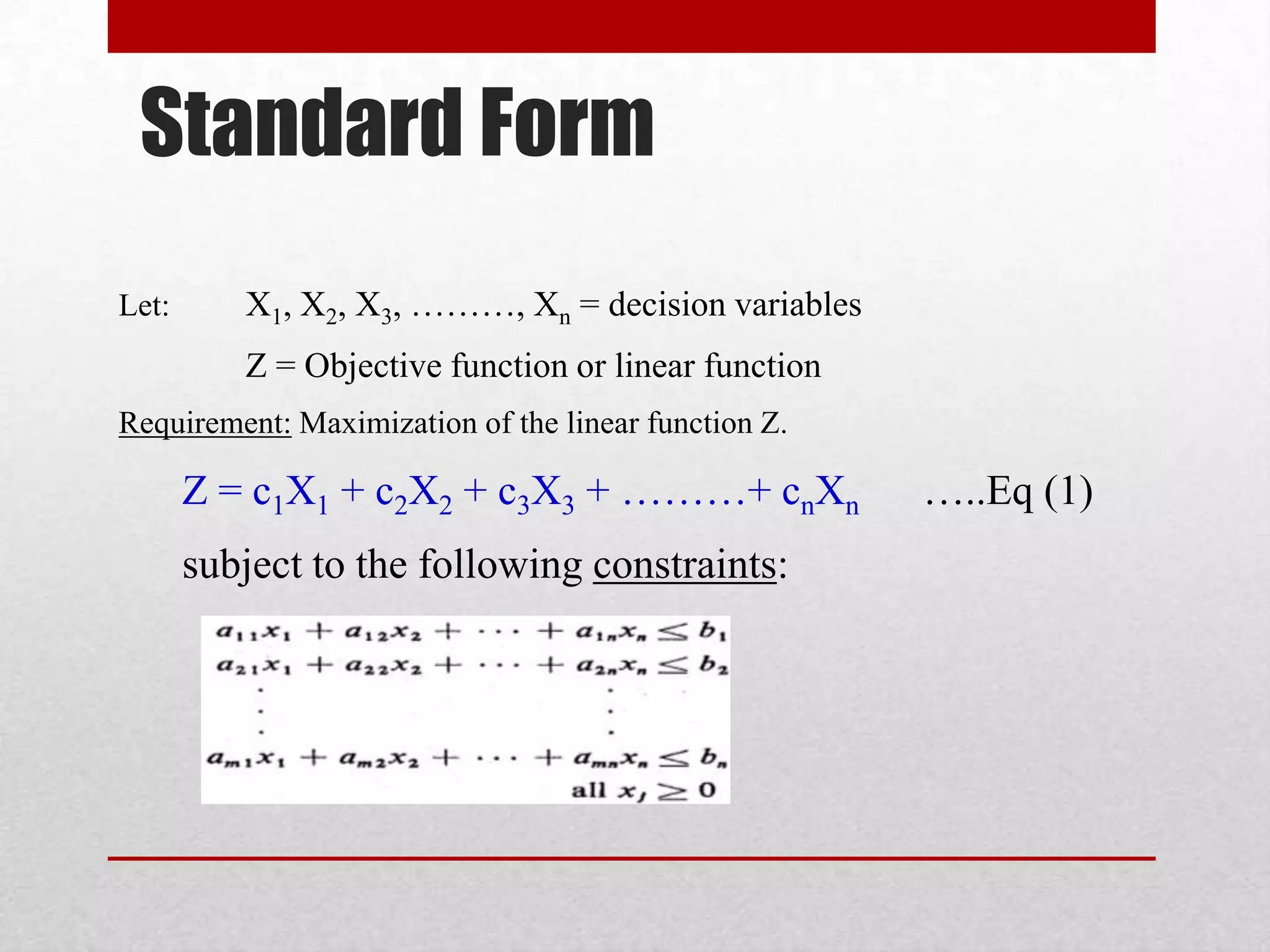
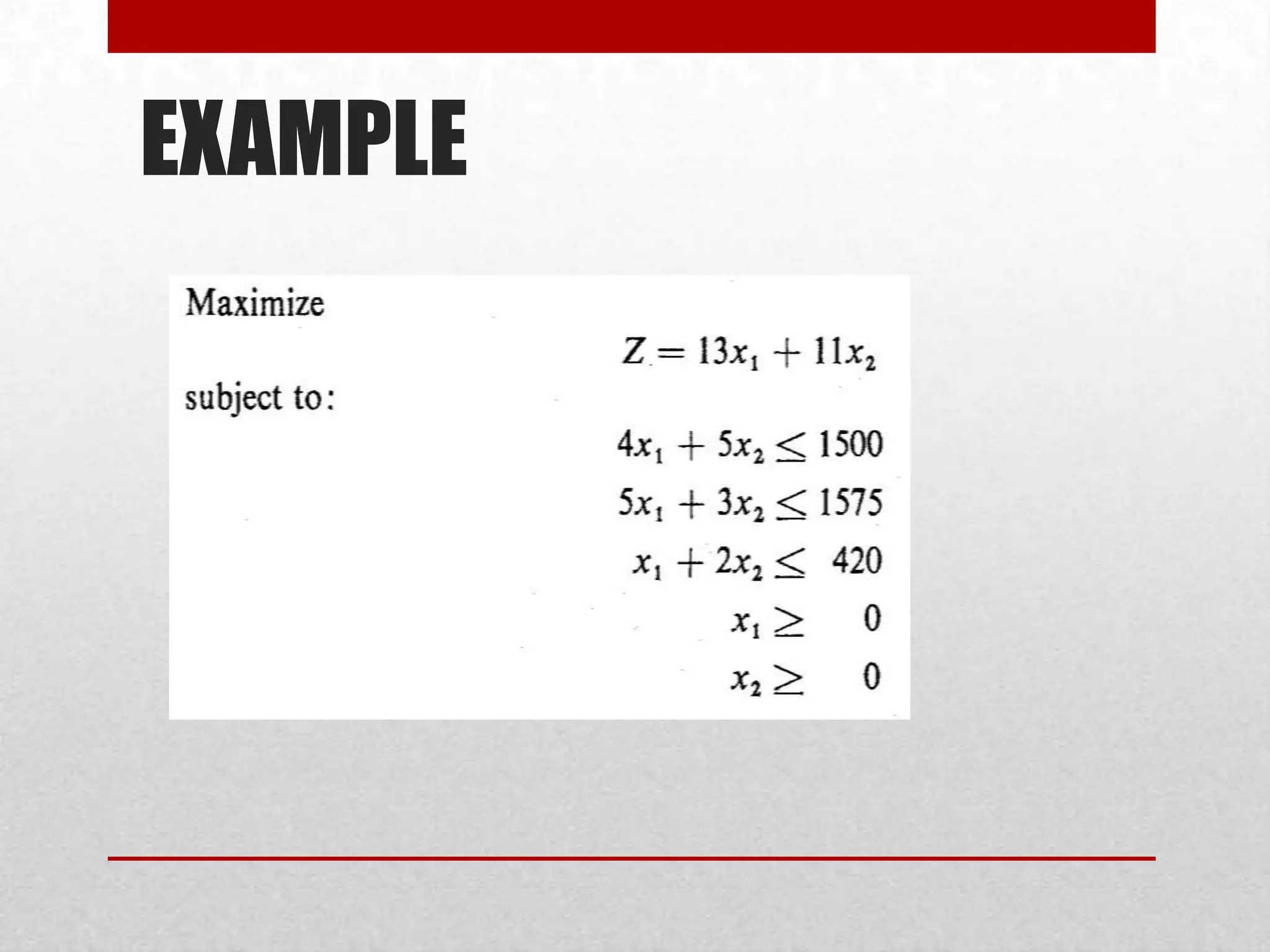
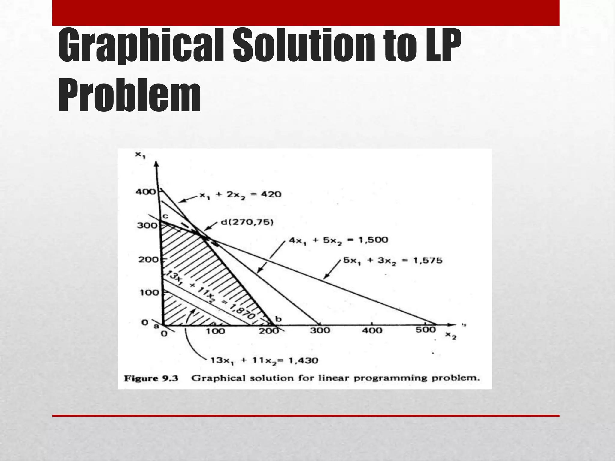
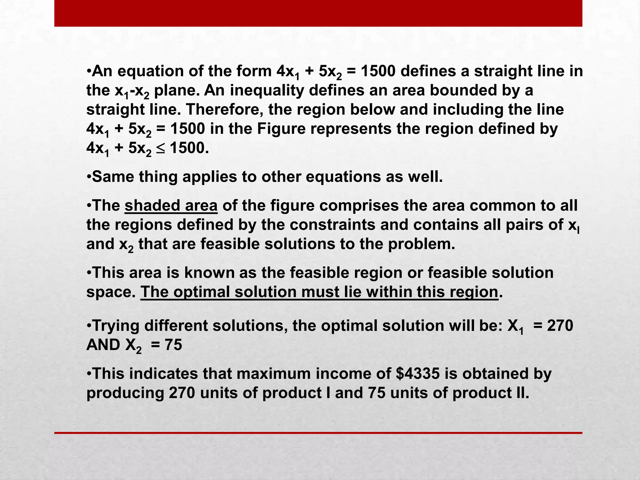
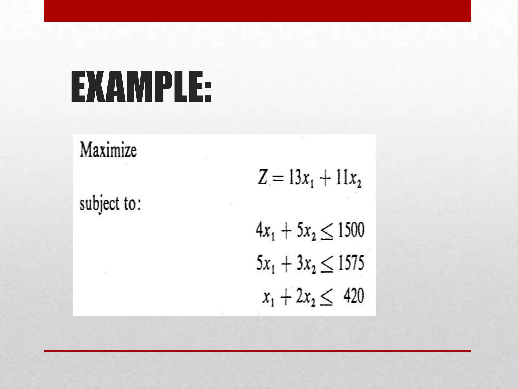
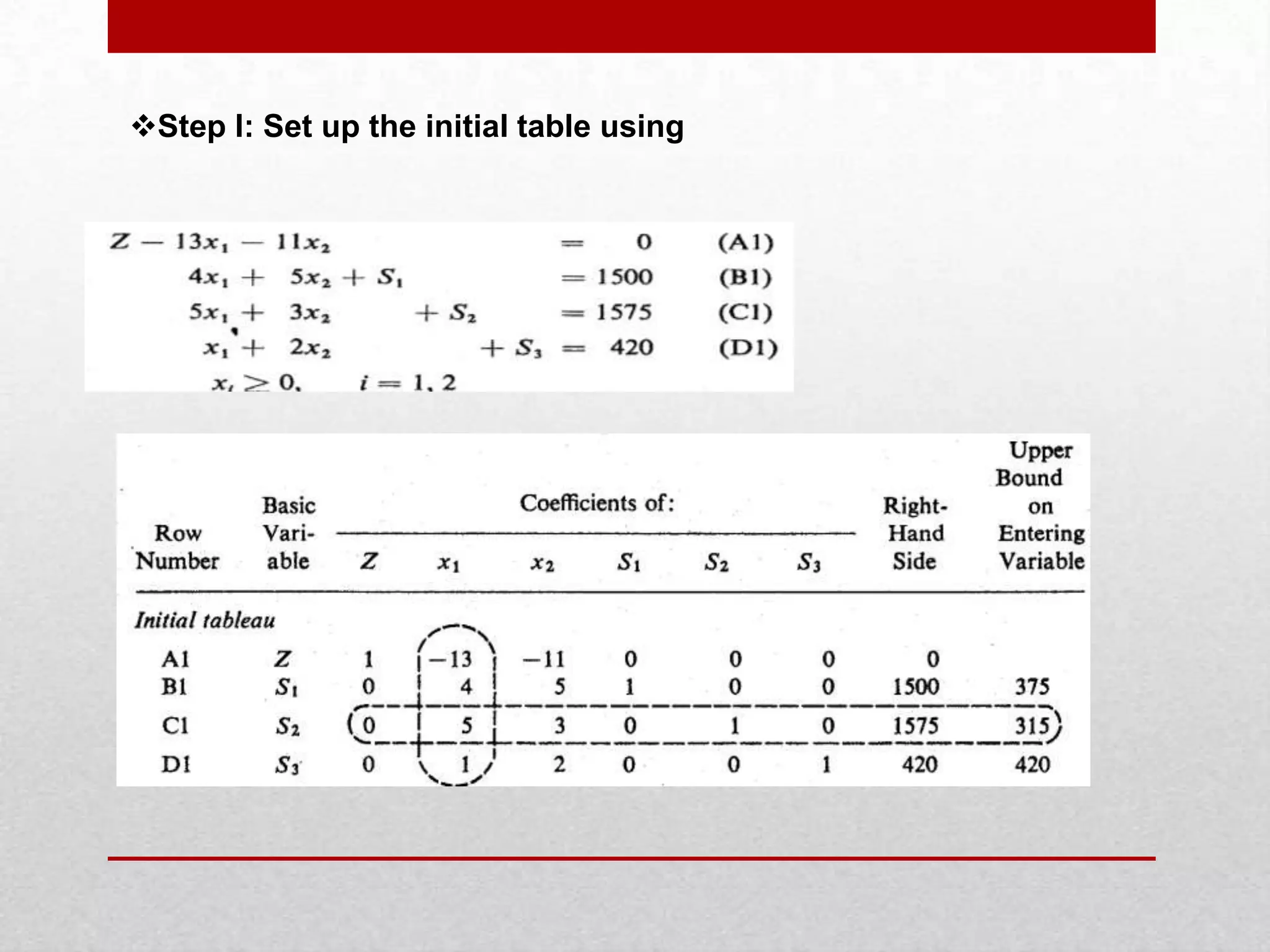
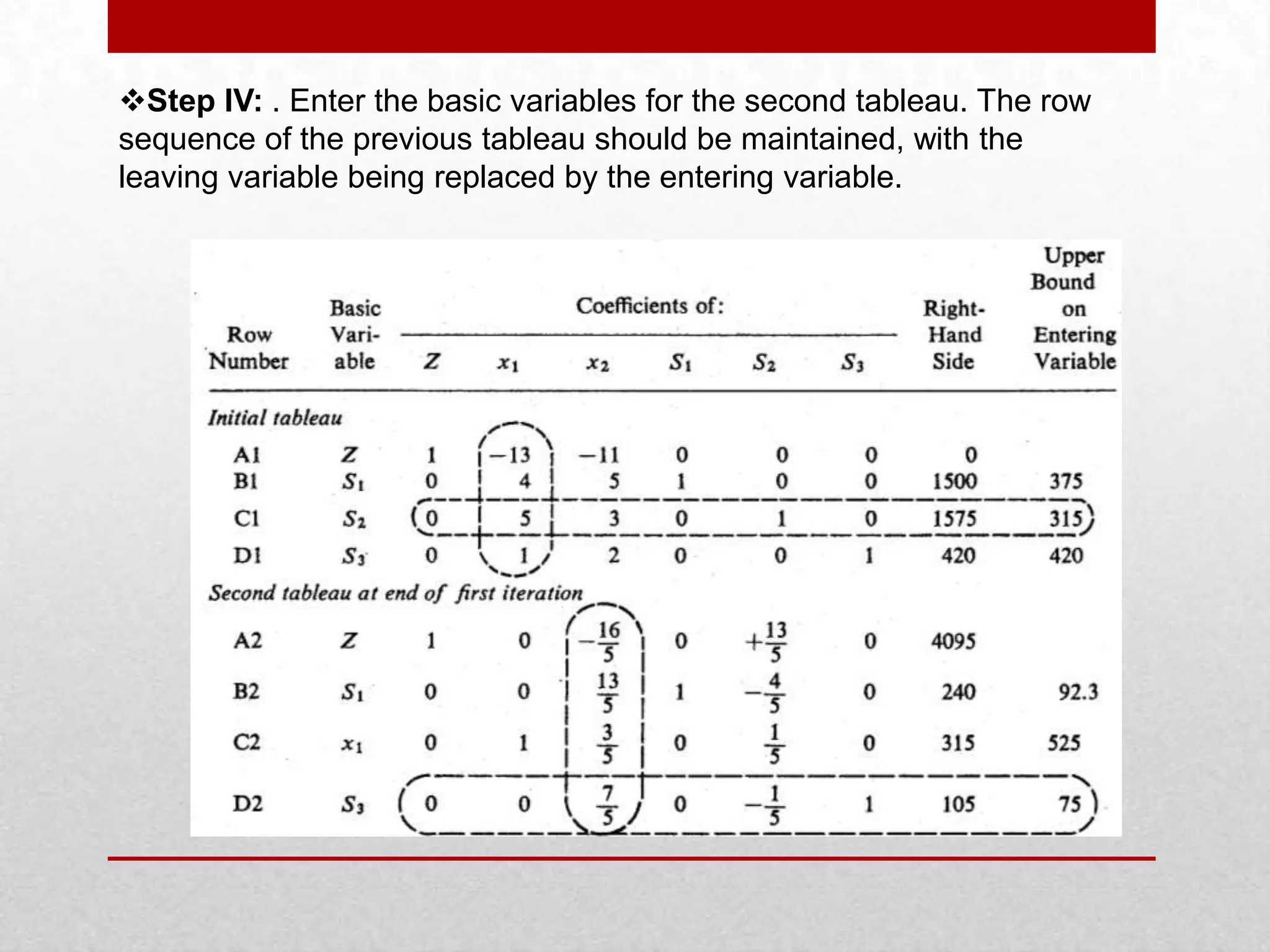
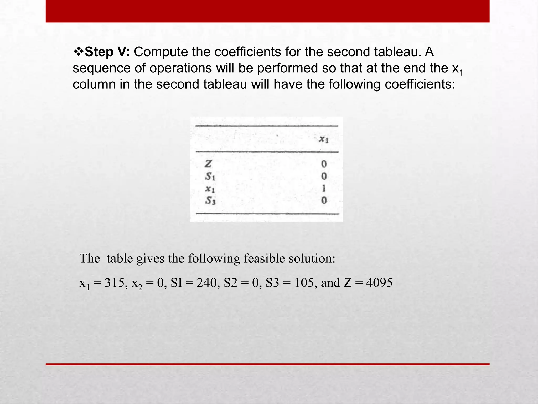
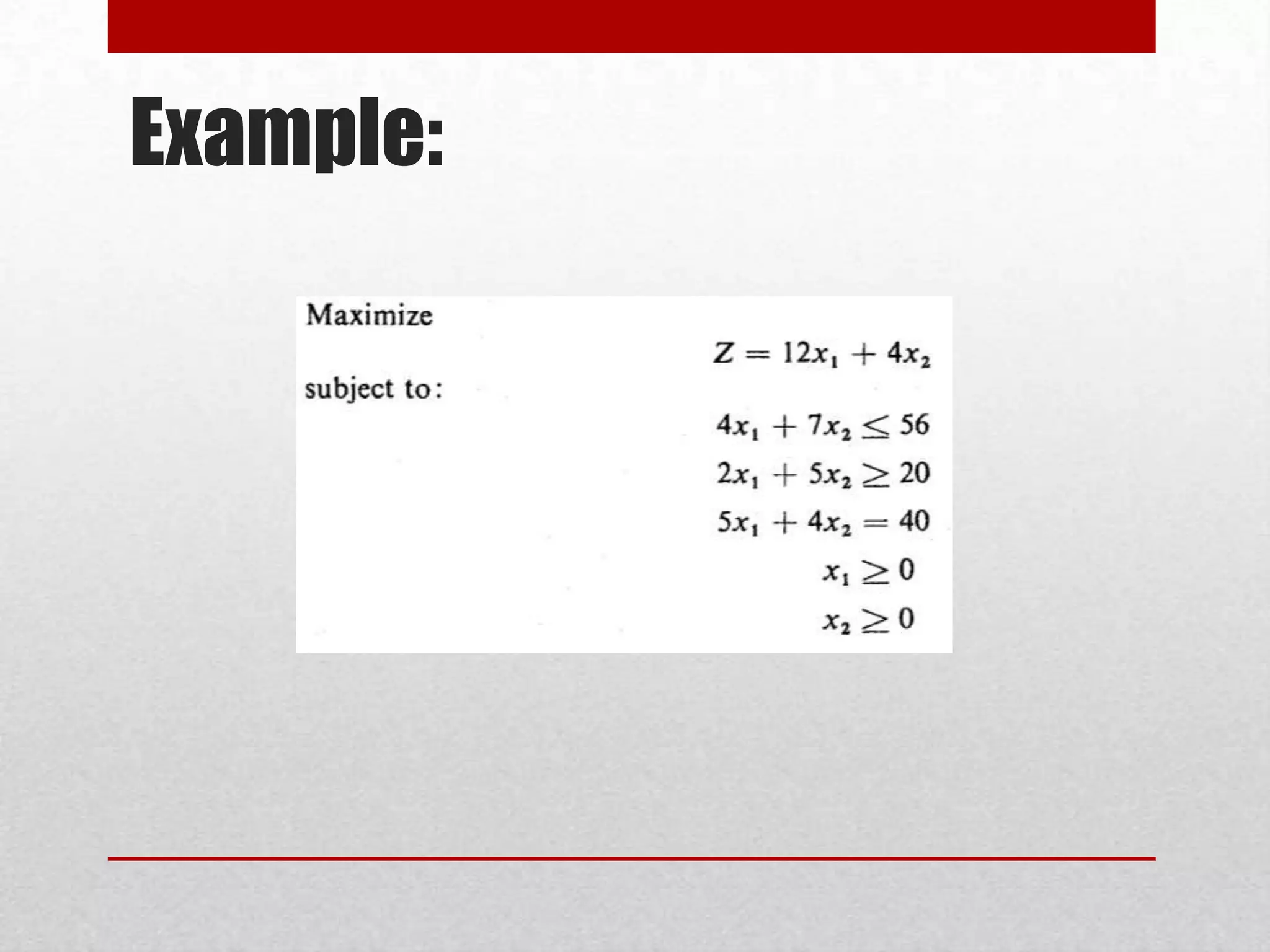
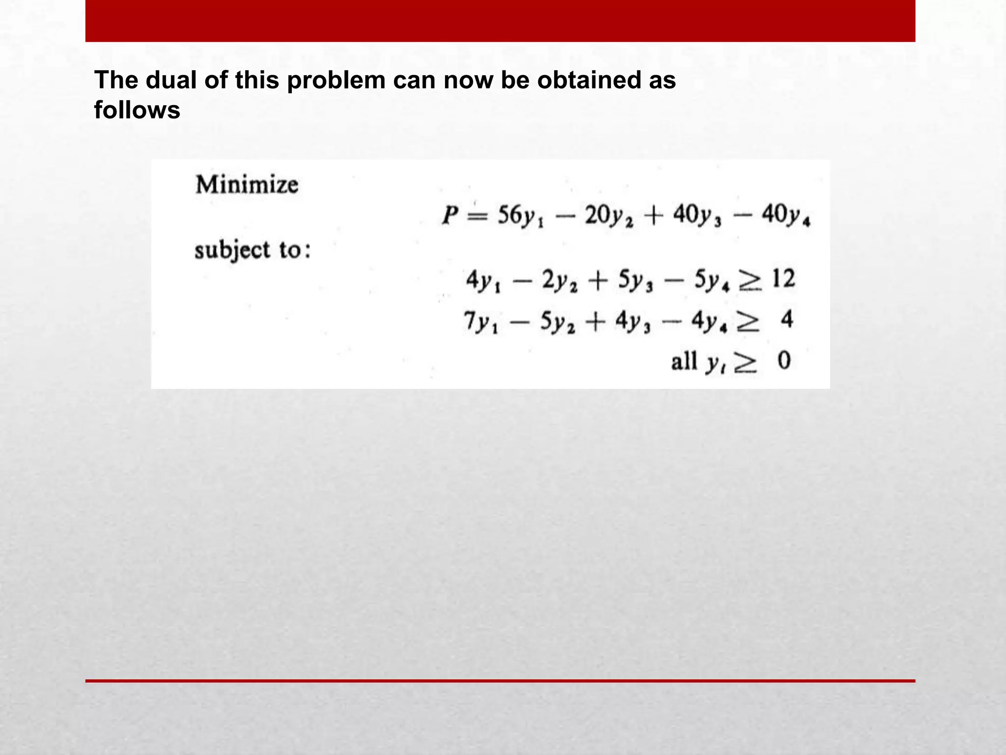
The document discusses linear programming, which is a technique for solving optimization problems with linear objective functions and constraints. It provides the standard form of a linear programming problem involving decision variables, an objective function to maximize, and constraints. Examples of both a graphical and algebraic (simplex method) solution are presented. The key concepts of feasible region, optimal solution, entering and leaving variables in the simplex method are explained. Duality, where every linear programming problem has an associated dual problem, is also introduced.

1. LINEAR
PROGRAMMING
SUBMITTED BY:
JASJEET KAUR
A1000702021
MCA 2A

2. What is Linear Programming?
• Linear programming (LP) refers to a
technique to solve a specific class of
mathematical optimization problems.
• LP optimization problems have linear
objective functions and constraints

3. Standard Form
Let:
X1, X2, X3, ………, Xn = decision variables
Z = Objective function or linear function
Requirement: Maximization of the linear function Z.
Z = c1X1 + c2X2 + c3X3 + ………+ cnXn
subject to the following constraints:
…..Eq (1)

4. EXAMPLE

5. Graphical Solution to LP
Problem

6. •An equation of the form 4x1 + 5x2 = 1500 defines a straight line in
the x1-x2 plane. An inequality defines an area bounded by a
straight line. Therefore, the region below and including the line
4x1 + 5x2 = 1500 in the Figure represents the region defined by
4x1 + 5x2  1500.
•Same thing applies to other equations as well.
•The shaded area of the figure comprises the area common to all
the regions defined by the constraints and contains all pairs of xI
and x2 that are feasible solutions to the problem.
•This area is known as the feasible region or feasible solution
space. The optimal solution must lie within this region.
•Trying different solutions, the optimal solution will be: X1 = 270
AND X2 = 75
•This indicates that maximum income of $4335 is obtained by
producing 270 units of product I and 75 units of product II.

7. The Simplex Method
When decision variables are more than 2, it is always
advisable to use Simplex Method to avoid lengthy
graphical procedure.
The simplex method is not used to examine all the
feasible solutions.
It deals only with a small and unique set of feasible
solutions, the set of vertex points (i.e., extreme points)
of the convex feasible space that contains the optimal
solution.

8. EXAMPLE:

9. Step I: Set up the initial table using

10. Step II: . Identify the variable that will be assigned a nonzero
value in the next iteration so as to increase the value of the
objective function. This variable is called the entering variable.
It is that nonbasic variable which is associated with the
smallest negative coefficient in the objective function.
If two or more nonbasic variables are tied with the smallest
coefficients, select one of these arbitrarily and continue
Step III: Identify the variable, called the leaving
variable, which will be changed from a nonzero to a zero
value in the next solution.

11. Step IV: . Enter the basic variables for the second tableau. The row
sequence of the previous tableau should be maintained, with the
leaving variable being replaced by the entering variable.

12. Step V: Compute the coefficients for the second tableau. A
sequence of operations will be performed so that at the end the x1
column in the second tableau will have the following coefficients:
The table gives the following feasible solution:
x1 = 315, x2 = 0, SI = 240, S2 = 0, S3 = 105, and Z = 4095

13. Duality
With every linear programming
problem, there is associated another linear
programming problem which is called the
dual of the original (or the primal) problem.

14. Example:

15. The dual of this problem can now be obtained as
follows